Bayesian Inference

1. Why Bayesian inference?

We will spend twelve sections building up the prior–likelihood–posterior framework. Before we touch a single equation, let’s say why anyone bothers.

1.1 The three angles

Three motivations recur across the Bayesian literature, and we’ll keep coming back to them.

Prior information. When we know something before we collect data — from physics, from previous studies, from a colleague’s lab notebook — Bayesian inference gives us a principled place to put it. The prior $\pi(\theta)$ encodes what we believed about $\theta$ before this dataset arrived. With a few hundred observations on a hard inference problem, the prior often makes the difference between a posterior that says something useful and one that says “either everything is possible or nothing is.” Frequentist methods can sometimes back this in via regularization — ridge regression has a Gaussian-prior reading, the lasso has a Laplace-prior reading — but the Bayesian frame makes the move explicit rather than tacit.

Calibrated uncertainty. A Bayesian estimator is a full posterior distribution, not a single number. The posterior carries the answers to questions a point estimate cannot: how wide is the credible interval, how much mass sits above some threshold, what is the posterior probability that $\theta$ lies in some region. For decisions that depend on tail behavior — does the new drug help more than 50% of patients, will the bridge hold under a 100-year load — uncertainty is the answer, not a decoration on it.

Decision-theoretic optimality. Once we have a posterior and a loss function, the Bayes-optimal decision rule is the one that minimizes posterior expected loss. This is a theorem (we’ll meet it in §7), and it is the cleanest existing answer to the question “given what I now believe, what should I do?” Frequentist decision theory exists and works, but it operates on the joint distribution of $(\theta, y)$ before $y$ is observed; the Bayesian version conditions on the observed $y$ and integrates over the parameter, which is usually what a working data scientist actually wants.

1.2 Motivating vignette: a Beta–Binomial A/B test

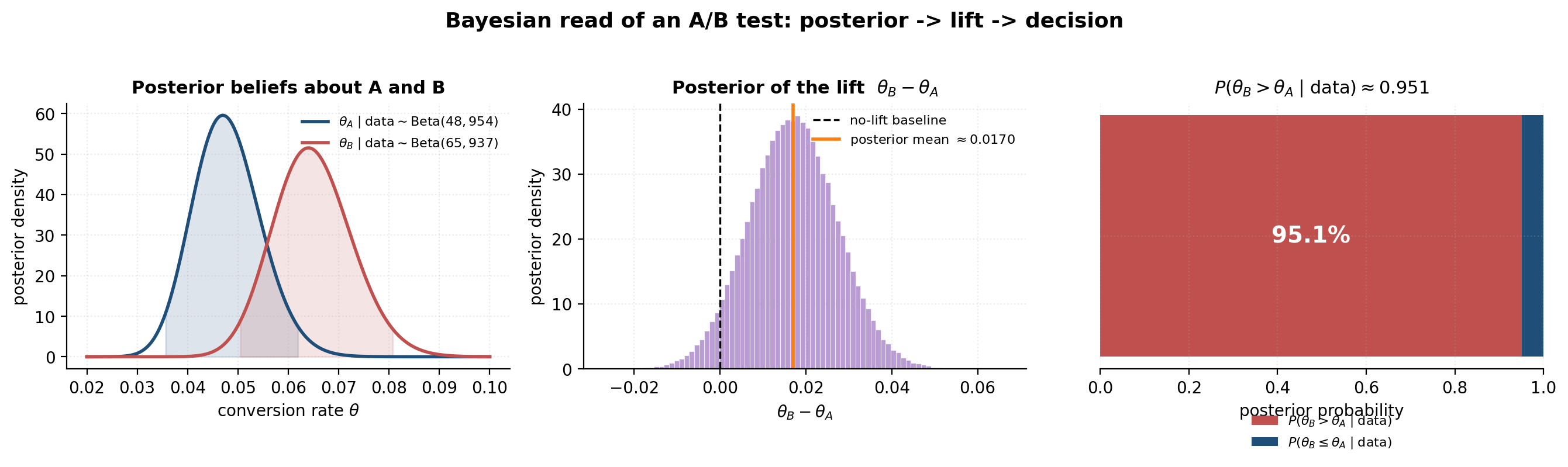
Throughout this topic we’ll return to a single concrete setup. We run 1000 impressions of variant A on a web page and observe 47 conversions; 1000 impressions of variant B and observe 64. Did B beat A?

The frequentist reflex is a two-proportion $z$-test. We get a $p$-value, possibly reject the null of equality, and report a confidence interval on $\theta_B - \theta_A$. The Bayesian reflex is different. We put a prior on each rate — a uniform $\mathrm{Beta}(1, 1)$, encoding “we have no idea before the data” — and compute the posteriors directly. Conjugacy (which we’ll prove in §4.2) gives us $\theta_A \mid \text{data} \sim \mathrm{Beta}(48, 954)$ and $\theta_B \mid \text{data} \sim \mathrm{Beta}(65, 937)$. From there we can ask any question we want.

The question that matters is: what is the posterior probability that B beats A? Monte Carlo answers it in three lines of code — draw 200,000 samples from each posterior, compute the differences, count the fraction that are positive. The answer is approximately $0.95$. That number is not a $p$-value — it is not a probability about a hypothetical infinite sample of replications — it is a probability about $\theta_B - \theta_A$ given the data we actually have.

1.3 What the umbrella does

The Bayesian framework is large enough that thirteen other formalML topics in T5 (Bayesian & Probabilistic ML) treat specific pieces of it in depth: variational inference, Gaussian processes, probabilistic programming, mixed-effects models, stacking and predictive ensembles, Bayesian neural networks, variational Bayes for model selection, sparse Bayesian priors, meta-learning, stochastic-gradient MCMC, sequential Monte Carlo, reversible-jump MCMC, and Riemann-manifold HMC. All thirteen are already shipped.

This topic’s job is to be the map. We introduce the vocabulary — prior, likelihood, posterior, posterior predictive, marginal likelihood, Bayes risk — and we forward-point. When we mention the ELBO, we name it as the variational approximation to the marginal likelihood and we link to variational inference; we do not re-derive the ELBO. When we mention NUTS, we say “Hamiltonian Monte Carlo with adaptive tree-depth tuning” and we link to probabilistic programming for the runnable code; we do not re-derive the leapfrog integrator. The umbrella’s value is coherence — the same framework underwrites all thirteen — not coverage.

1.4 Roadmap

§2 puts the framework on paper: the joint distribution viewpoint, Bayes’ theorem, the marginal-likelihood normalizer. §3 discusses what goes into the prior — informative, uninformative, Jeffreys, reference. §4 catalogs the conjugate families that give closed-form posteriors and proves the Beta–Binomial result the A/B-test rests on. §5–§7 cover what comes out of a posterior: point estimates, predictive distributions, optimal decisions. §8 elaborates on sequential updating and exchangeability. §9 brings in hierarchy and shrinkage. §10 covers Bayesian model comparison. §11 surveys the computational landscape when conjugacy fails, with forward-pointers to every relevant T5 leaf. §12 is the frequentist–Bayesian dialogue and the Bernstein–von Mises bridge. §13 marks the scope honestly — what’s outside the umbrella’s range.

2. The prior–likelihood–posterior cycle

A Bayesian model is a joint probability distribution. That’s the whole content of this section, restated in a few different ways until the joint-distribution viewpoint clicks. Once it does, the rest of the topic — point estimates, posterior predictives, decision rules, hierarchical models — is just various ways of slicing or summarizing the joint.

2.1 The joint distribution viewpoint

Suppose we have a parameter $\theta \in \Theta$ (unobserved, what we want to learn about) and data $y \in \mathcal{Y}$ (observed). A Bayesian model is a joint distribution $p(\theta, y)$ on $\Theta \times \mathcal{Y}$. The chain rule of probability gives us two factorizations of that joint:

$p(\theta, y) \;=\; \pi(\theta)\, p(y \mid \theta) \;=\; \pi(\theta \mid y)\, p(y).$

The left factorization is how we build the model: write down what we believed about $\theta$ before any data (the prior $\pi(\theta)$), then write down how $y$ is generated from $\theta$ (the likelihood $p(y \mid \theta)$). The right factorization is how we use the model after $y$ is observed: the marginal density $p(y)$ tells us how surprising the data are under our prior beliefs, and the conditional density $\pi(\theta \mid y)$ tells us what we now believe about $\theta$ in light of $y$ — the posterior.

Equating the two factorizations gives Bayes’ theorem.

2.2 Bayes’ theorem (continuous form)

This is the equation that does all the work. The discrete analog — with sums replacing the integral and probabilities replacing densities — is what we saw in introductory probability courses; the continuous version is the direct analog at the level of densities. A measure-theoretic statement adds the Radon-Nikodym derivative formalism, which we don’t need here.

2.3 Proof of Bayes’ theorem

The proof is one line of algebra. Its weight is entirely in the renaming that follows it.

The renaming move. That’s it. Two lines of algebra. The pedagogically load-bearing move is what we now choose to call each piece. Take a long look at the equation $\pi(\theta \mid y) = p(y \mid \theta) \pi(\theta) / p(y)$. Every component has a name, and the names tell the story of an entire research program.

The prior $\pi(\theta)$ is what we believed about $\theta$ before $y$ arrived. It carries background knowledge — physics, previous experiments, the opinion of a domain expert, the assumption that the parameter is unlikely to be ridiculous. §3 discusses where it comes from.

The likelihood $p(y \mid \theta)$ is the data-generating distribution, read as a function of $\theta$ for fixed observed $y$. It is not a probability density in $\theta$ — it does not integrate to one over $\Theta$ — but it is the only place in the equation where the observed $y$ enters. Everything we learn from $y$ comes through the likelihood.

The posterior $\pi(\theta \mid y)$ is our updated belief about $\theta$ after seeing $y$. It is a probability density in $\theta$ (it does integrate to one over $\Theta$), and it is the deliverable of Bayesian inference. Every quantity we compute in §5–§7 — point estimates, credible intervals, predictive distributions, decisions — is a functional of the posterior.

The marginal likelihood (or evidence) $p(y)$ is the probability of the observed data, averaged over the prior. It plays two roles. As a normalizing constant it makes the posterior integrate to one. As a model-comparison quantity it tells us how surprised we should be by $y$ under our chosen model, which is the foundation for Bayes factors (§10).

The discipline is to think of the cycle running in both directions. Forward, from prior and likelihood, the model declares a joint distribution. Backward, conditioning on observed $y$, the same joint distribution coughs up a posterior. Bayes’ theorem is the symmetric statement that the same joint, read two ways, must agree.

The interactive below lets you set the prior parameters $(\alpha, \beta)$ and the data $(n, s)$ and watch the prior, the (rescaled) likelihood, and the resulting posterior react. Default state: $\alpha = \beta = 1$ (flat prior), $n = 1000$, $s = 47$ (A/B-test variant A). Dragging the prior sliders toward more concentrated values pulls the posterior toward the prior; dragging $n$ up at fixed $s/n$ tightens the posterior around the MLE regardless of the prior. The visual feeling — with little data the prior dominates; with lots of data the likelihood dominates — is the load-bearing intuition for §3.

α (prior pseudo-successes + 1): 1.0β (prior pseudo-failures + 1): 1.0n (trials): 1000s (successes): 47

2.4 The marginal likelihood, and why we often ignore it

Computing $p(y) = \int p(y \mid \theta) \pi(\theta) d\theta$ is the hard part of Bayesian inference. For conjugate models (§4) the integral has a closed form. For nonconjugate models it usually doesn’t, and an enormous fraction of Bayesian computation (variational inference, MCMC, SMC) exists to dodge that integral.

For most posterior-shape questions we don’t need to. Notice that $p(y)$ is a constant — it does not depend on $\theta$ — so

$\pi(\theta \mid y) \;\propto\; p(y \mid \theta) \, \pi(\theta).$

Up to proportionality, the posterior is just likelihood times prior. We can find the posterior mode (MAP), sample from the posterior (MCMC), or fit a variational approximation (VI) using only the unnormalized $p(y \mid \theta) \pi(\theta)$ — the normalizing constant cancels out. This is why MCMC algorithms can sample from a distribution whose density they cannot compute in closed form.

When does $p(y)$ matter? Two contexts. First, model comparison (§10): the Bayes factor $B_{12} = p(y \mid M_1) / p(y \mid M_2)$ is a ratio of marginal likelihoods, and the marginal likelihoods themselves carry the information. Second, marginal-likelihood-based predictive scoring in certain settings. Otherwise, treat $p(y)$ as bookkeeping.

2.5 Numerical sanity check on a finite joint table

Before we move to continuous examples, it’s worth verifying the algebra on a discrete joint distribution where every step can be checked by hand. The canonical example is medical testing.

Suppose 1% of a population has a disease (so $P(D) = 0.01$ is the prior). A test is 99% sensitive ($P(T+ \mid D) = 0.99$) and 95% specific ($P(T- \mid \neg D) = 0.95$). A patient tests positive — what is the posterior probability they have the disease?

The notebook builds the $2 \times 2$ joint table, computes the marginal $P(T+)$ from row sums, and confirms that two routes to $P(D \mid T+)$ — direct from the joint table, and via Bayes’ theorem — agree to floating-point precision. The answer is about $0.167$: even with a 99%-sensitive test, the posterior probability of disease given a positive result is only about 17%, because the prior is so concentrated on the no-disease event. The prior matters, especially for rare events. This small calculation is also the workhorse pedagogical example for the broader literature on base-rate neglect.

3. Choosing a prior

If the posterior depends on the prior, where does the prior come from? This is the awkward question Bayesian inference forces us to answer. We handle it in three layers: an informative prior carries explicit subjective belief (§3.1); an uninformative prior tries to avoid carrying any, with the catch that “no information” is parameterization-dependent (§3.2–§3.3); and a reference prior is the mathematically-honest version of “uninformative” for problems where Jeffreys isn’t enough (§3.4). Underneath all of them is a rule of thumb that resolves most arguments: with enough data, the prior washes out (§3.5).

3.1 Subjective informativeness and pseudo-counts

The cleanest way to think about a Beta prior is via pseudo-counts. A $\mathrm{Beta}(\alpha, \beta)$ distribution behaves, when used as a prior for a Binomial rate, as if we had already observed $(\alpha - 1)$ pseudo-successes and $(\beta - 1)$ pseudo-failures from a previous experiment.

To see this, write the prior density up to its normalizing constant: $\pi(\theta) \propto \theta^{\alpha - 1}(1 - \theta)^{\beta - 1}$. The Binomial likelihood is $p(s \mid \theta) \propto \theta^s (1 - \theta)^{n - s}$, where $s$ is observed successes in $n$ trials. The product — which is proportional to the posterior — has exponents $(\alpha + s - 1)$ and $(\beta + n - s - 1)$. The prior simply added $(\alpha - 1, \beta - 1)$ to the data exponents. That’s the entire content of conjugacy from the counting viewpoint.

So $\mathrm{Beta}(1, 1)$ — the uniform prior — corresponds to “zero pseudo-successes, zero pseudo-failures.” $\mathrm{Beta}(20, 80)$ is “19 pseudo-successes, 79 pseudo-failures, suggesting a rate near 0.2.” $\mathrm{Beta}(0.5, 0.5)$ — the Jeffreys prior we’ll meet in §3.3 — is ”$-0.5$ pseudo-successes and $-0.5$ pseudo-failures,” which is a fine prior (the Beta density is well-defined for all positive parameters) but a strained pseudo-count interpretation; the §3.3 invariance argument is what justifies using it anyway.

The reason this interpretation is so useful is that conjugacy turns it into bookkeeping. The posterior after observing $s$ successes in $n$ trials is

$\pi(\theta \mid \text{data}) \;=\; \mathrm{Beta}(\alpha + s, \, \beta + n - s),$

which we read as “prior pseudo-successes plus observed successes, prior pseudo-failures plus observed failures.” A prior with $\alpha + \beta = 100$ is “worth” 100 observations of data; a prior with $\alpha + \beta = 2$ is “worth” 2. This is the gold-standard intuition for prior strength.

The elicitation interview, then, is: “Suppose you were going to write down a Beta prior on this rate. How many fake-data observations is your prior worth? And where do you think the rate sits?” Once you’ve answered both, you have $\alpha + \beta$ (total pseudo-count) and $\alpha / (\alpha + \beta)$ (prior mean), which uniquely identifies $\alpha$ and $\beta$.

3.2 Uniform and weakly informative defaults

The reflex on hearing “I have no prior information” is to declare a uniform prior. For a Binomial rate, this is $\mathrm{Beta}(1, 1)$ — flat on the unit interval. For a Gaussian mean, it would be an (improper) flat prior on the real line. Uniform priors are tempting because they look objective — every value of $\theta$ is equally probable.

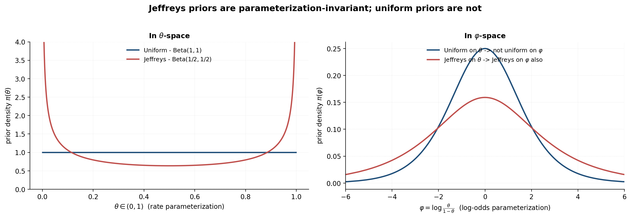
The catch is that uniform-on-$\theta$ is not uniform-on-$\varphi$ for any reparameterization $\varphi = g(\theta)$. If our parameter is a rate $\theta \in (0, 1)$, the natural reparameterization for logistic regression is the log-odds $\varphi = \log(\theta / (1 - \theta)) \in \mathbb{R}$. A uniform prior on $\theta$ implies a non-uniform prior on $\varphi$ (specifically the logistic distribution), and vice versa. We cannot be uninformative in both parameterizations at once. The choice of parameterization smuggles in prior information, even when the prior looks “flat.” The figure for §3.3 makes this concrete.

The pragmatic response is to use weakly informative priors — distributions diffuse enough to let the data dominate quickly, but informative enough to exclude obviously-implausible regions. For a probability, $\mathrm{Beta}(2, 2)$ is a standard weakly informative choice — flat-ish, centered at $0.5$, ruling out the extremes. For a regression coefficient with no other information, a $\mathcal{N}(0, 5^2)$ prior is the standard recommendation: nonzero variance, no specific claim about the sign, ruling out coefficients of magnitude greater than ~15 a priori. The Gelman group’s Bayesian Data Analysis (BDA3) is the canonical reference for these defaults.

3.3 Jeffreys priors

The most-principled answer to “what is an uninformative prior?” is Harold Jeffreys’s 1946 invariance argument. Pick the prior whose density is proportional to the square root of the Fisher information:

$\pi_J(\theta) \;\propto\; \sqrt{I(\theta)}, \qquad I(\theta) \;=\; -\mathbb{E}_{\theta}\!\left[\frac{\partial^2 \log p(y \mid \theta)}{\partial \theta^2}\right].$

The motivation is reparameterization invariance. If we transform $\theta \to \varphi = g(\theta)$, the Fisher information transforms as $I_\varphi(\varphi) = I_\theta(\theta) \, (d\theta/d\varphi)^2$, which means the Jeffreys prior transforms with the same Jacobian — so $\pi_J(\varphi)$ computed in the $\varphi$-parameterization is consistent with transforming $\pi_J(\theta)$ under the change of variables. Jeffreys is the unique (up to scale) prior that is invariant under reparameterization.

Jeffreys prior for the Binomial rate. The Fisher information for $n$ i.i.d. $\mathrm{Bernoulli}(\theta)$ observations is $I(\theta) = n / (\theta(1 - \theta))$. So

$\pi_J(\theta) \;\propto\; \sqrt{\frac{1}{\theta(1 - \theta)}} \;=\; \theta^{-1/2}(1 - \theta)^{-1/2},$

which is the kernel of $\mathrm{Beta}(1/2, 1/2)$. The Jeffreys prior is U-shaped — it puts more mass near 0 and 1 than near 0.5. That’s surprising, but it’s the price of invariance. Note that $\mathrm{Beta}(1/2, 1/2)$ is a proper prior (it integrates to 1 like any Beta with positive parameters) even though its pseudo-count reading ($-1/2$ pseudo-successes, $-1/2$ pseudo-failures) is physically nonsense.

For multidimensional parameters and irregular likelihoods, Jeffreys priors get harder to compute and sometimes give unappealing results — for the multivariate Normal, for example, the joint Jeffreys prior differs from the “independent Jeffreys on each component” prior. Jeffreys is a tool, not an algorithm.

3.4 Reference priors and the limits of “objectivity”

Bernardo’s 1979 reference prior program is the formal generalization of Jeffreys to multidimensional parameters. The idea is to choose the prior that maximizes the asymptotic information gain — the prior under which the posterior, on average over data, diverges from the prior as much as possible in a KL-divergence sense. For one-dimensional regular models the reference prior coincides with Jeffreys; for multidimensional models with a designated parameter-of-interest and nuisance parameters, the reference prior orders the parameters and computes a sequence of conditional Jeffreys priors. The full construction is in Bernardo & Smith (1994); the umbrella forward-points rather than develops it.

The honest summary is this: no prior is no opinion. Every choice of prior — uniform, weakly informative, Jeffreys, reference, expert-elicited — encodes a position about which parameter values are a priori plausible. The Bayesian frame forces us to make that position explicit. Frequentist methods often have implicit priors — the lasso has a Laplace prior, ridge has a Gaussian prior, the MLE corresponds to a uniform improper prior — but those priors are not declared, debated, or sensitivity-checked. The Bayesian discipline is to declare the prior, then check whether the answer is sensitive to it.

3.5 When the prior dominates, when it washes out

The Beta–Binomial conjugacy formula $\mathrm{Beta}(\alpha + s, \beta + n - s)$ tells the whole story in one line. The posterior is determined by pseudo-counts plus data counts. As long as the data counts dominate the prior pseudo-counts — $s \gg \alpha$ and $n - s \gg \beta$ — the posterior is dominated by the likelihood and the prior choice doesn’t matter much.

A heuristic that resolves most arguments: if your prior pseudo-count $\alpha + \beta$ is small compared to your sample size $n$, there is nothing to argue about. If $\alpha + \beta$ is comparable to $n$, there is — and the right move is to run a sensitivity analysis (does the posterior change meaningfully under a different prior?) and report the result.

Asymptotically (§12, Bernstein–von Mises) the posterior concentrates at the MLE with variance $\sim 1/(n I(\hat\theta))$, and the prior contributes a vanishing $O(1/n)$ correction. For an A/B test with $n$ in the thousands, the prior is bookkeeping; for an inference problem with $n$ in the dozens, it isn’t.

The interactive below lets the reader sweep the sample size $n$ at a fixed ratio $s/n \approx 0.047$ and watch three different priors — uniform $\mathrm{Beta}(1, 1)$, weakly informative $\mathrm{Beta}(2, 2)$, strongly (and deliberately wrongly) informative $\mathrm{Beta}(20, 80)$ — converge to the same posterior as $n$ grows. The top row of priors stays fixed; the bottom row shows the posteriors at the chosen $n$.

n (large-sample row): 1000 (s = 47, s/n ≈ 0.047)

Black dashed line: posterior mean. Gray dotted line: empirical MLE s/n ≈ 0.047. As n grows, the three columns' posteriors converge toward the MLE — the prior washes out.

4. Conjugate families

A conjugate prior is a prior whose functional form is preserved by the posterior update: prior in some parametric family, observe data, get a posterior in the same parametric family with updated parameters. When this happens, the posterior has a closed form and Bayesian inference reduces to bookkeeping on the prior’s parameters.

Conjugacy is a small miracle — it shouldn’t generically work, but it does for an important catalog of likelihood-prior pairs. The reason is structural: every conjugate pair is an instance of the exponential-family construction we’ll meet in §4.5. The umbrella owns one full proof here (the Beta–Binomial result our A/B-test running example rests on); everything else is sketched and pointed to the literature.

4.1 Definition: stability under the posterior update

A family $\mathcal{F} = \{\pi(\theta \mid \boldsymbol{\eta}) : \boldsymbol{\eta} \in H\}$ of prior distributions, parameterized by hyperparameters $\boldsymbol{\eta}$, is conjugate for a likelihood $p(y \mid \theta)$ if, for every prior $\pi(\cdot \mid \boldsymbol{\eta}) \in \mathcal{F}$ and every observed $y$, the posterior $\pi(\theta \mid y, \boldsymbol{\eta})$ is also a member of $\mathcal{F}$:

$\pi(\theta \mid \boldsymbol{\eta}) \in \mathcal{F}, \quad p(y \mid \theta) \text{ a fixed likelihood} \quad \Longrightarrow \quad \pi(\theta \mid y, \boldsymbol{\eta}) = \pi(\theta \mid \boldsymbol{\eta}'(y)) \in \mathcal{F}$

for some updated hyperparameters $\boldsymbol{\eta}'(y)$ depending on the data. The update map $\boldsymbol{\eta} \to \boldsymbol{\eta}'(y)$ is what we call the “conjugate update rule,” and it usually has the flavor of counting: pseudo-counts in the prior plus observed counts from the data.

4.2 Beta–Binomial conjugacy (full proof)

This is the second of the umbrella’s two load-bearing proofs (the first was Bayes’ theorem, §2.3). The Beta–Binomial result is short but illustrative; it’s the template for every other conjugate pair in §4.4.

The combinatorial moral. Two ideas live inside this proof, and both matter for the rest of the topic.

First, conjugacy is closure under counting. The Beta family is “closed” under Binomial data: starting from any Beta prior and observing Binomial data, we always land back in the Beta family. The conjugate update rule is, mechanically, “add observed successes to $\alpha$, add observed failures to $\beta$.” Conjugacy turns Bayesian inference into bookkeeping.

Second, the pseudo-count interpretation is exact, not metaphorical. The prior $\mathrm{Beta}(\alpha, \beta)$ contributes $\alpha - 1$ pseudo-successes and $\beta - 1$ pseudo-failures to the posterior’s effective sample size. The numbers $\alpha + s$ and $\beta + n - s$ in the posterior’s parameters are literally “pseudo-counts plus observed counts.” This is why we said in §3.1 that “a Beta(20, 80) prior is worth 100 observations of data” — the total prior pseudo-count $\alpha + \beta$ is the prior’s effective sample size, and it lives on the same axis as the actual sample size $n$.

Applied to the A/B-test running example. With a uniform $\mathrm{Beta}(1, 1)$ prior on each rate and observed $(n, s) = (1000, 47)$ for variant A, the posterior is

$\theta_A \mid \text{data} \;\sim\; \mathrm{Beta}(1 + 47, \, 1 + 953) \;=\; \mathrm{Beta}(48, \, 954),$

with posterior mean $48 / 1002 \approx 0.0479$. For variant B with $(n, s) = (1000, 64)$, the posterior is $\mathrm{Beta}(65, 937)$ with posterior mean $65 / 1002 \approx 0.0649$. These are the posteriors we used in §1.2 and §2.2 without proof; now they’re earned.

The interactive below animates the conjugate update one observation at a time, drawing from $\mathrm{Bernoulli}(0.047)$. Posteriors are color-coded along a viridis gradient (light = early, dark = late). The true rate is marked. “Play” runs through all 1000 observations; “Reset” returns to $n = 0$; the slider jumps to any $n$.

PlayResetNew drawsn = 0, s = 0 → Beta(1, 1), mean = 0.5000

n (skip ahead): 0

4.3 Normal–Normal conjugacy (known variance)

The other workhorse conjugate pair is Normal–Normal, which underwrites most regression analysis and any inference about a mean. We state the result and sketch the proof; the algebra is “complete the square,” familiar from any treatment of the multivariate Gaussian.

The precision-weighting interpretation. Two readings of these formulas matter for downstream sections.

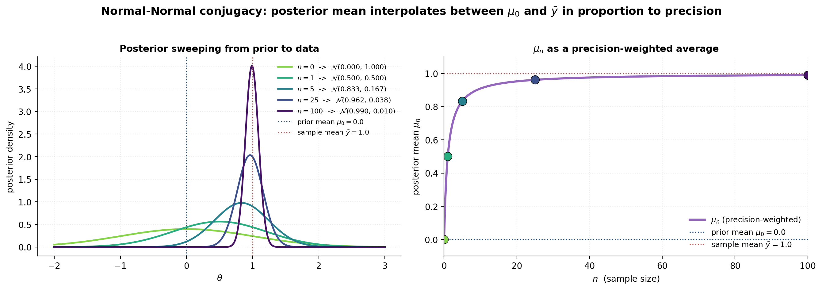
Precisions add. The Gaussian precision is the inverse of the variance, $1/\tau^2$. The conjugate Normal–Normal update says the posterior precision is the sum of the prior precision and the data precision $n/\sigma^2$. Information is additive on the precision scale, not the variance scale. This is the Gaussian analog of “pseudo-counts plus observed counts” — but where Beta–Binomial counts in successes, Gaussian counts in $n/\sigma^2$, which is the effective sample size on a unit-variance scale.

The posterior mean is a precision-weighted average. Rearranging,

$\mu_n \;=\; \frac{(1/\tau_0^2) \, \mu_0 + (n/\sigma^2) \, \bar y}{1/\tau_0^2 + n/\sigma^2}.$

The posterior mean is a convex combination of the prior mean $\mu_0$ and the sample mean $\bar y$, with weights proportional to their respective precisions. As $n \to \infty$, the data precision $n/\sigma^2 \to \infty$, the weight on $\bar y$ goes to 1, and $\mu_n \to \bar y$. As $n \to 0$, the data precision vanishes, and $\mu_n \to \mu_0$. The posterior interpolates between prior and data exactly in proportion to their relative information content.

This precision-weighted-average view is the right mental model for hierarchical Bayes (§9), where the same algebra gives partial pooling across groups: each group’s posterior mean is a precision-weighted average of the group’s own data and the global mean.

4.4 The closed-form catalog

Five conjugate pairs cover the bulk of practical Bayesian inference. Each follows the same template as Beta–Binomial: write the likelihood and the prior in their kernel-and-normalizer form, multiply, recognize the kernel of the same parametric family, read off the updated parameters.

Likelihood	Conjugate prior	Posterior update
$y \sim \mathrm{Binomial}(n, \theta)$	$\theta \sim \mathrm{Beta}(\alpha, \beta)$	$\mathrm{Beta}(\alpha + s, \, \beta + n - s)$
$y_i \sim \mathrm{Poisson}(\lambda)$	$\lambda \sim \mathrm{Gamma}(a, b)$ (shape, rate)	$\mathrm{Gamma}\bigl(a + \sum_i y_i, \, b + n\bigr)$
$y_i \sim \mathcal{N}(\mu, \sigma^2)$, $\sigma^2$ known	$\mu \sim \mathcal{N}(\mu_0, \tau_0^2)$	$\mathcal{N}(\mu_n, \tau_n^2)$ — see §4.3
$y_i \sim \mathcal{N}(\mu, \sigma^2)$, $\mu$ known	$\sigma^2 \sim \mathrm{Inv\text{-}Gamma}(a, b)$	$\mathrm{Inv\text{-}Gamma}\bigl(a + n/2, \; b + \tfrac{1}{2}\sum_i (y_i - \mu)^2\bigr)$
$\mathbf{y} \sim \mathrm{Multinomial}(n; \boldsymbol{\theta})$	$\boldsymbol{\theta} \sim \mathrm{Dirichlet}(\boldsymbol{\alpha})$	$\mathrm{Dirichlet}(\boldsymbol{\alpha} + \mathbf{y})$
$y_i \sim \mathcal{N}(\mu, \sigma^2)$, both unknown	$(\mu, \sigma^2) \sim \mathrm{NIG}(\mu_0, \kappa_0, a_0, b_0)$	$\mathrm{NIG}$ with updated parameters — see BDA3 §3.3

Gamma–Poisson is the count-data analog of Beta–Binomial. The Gamma prior on a Poisson rate $\lambda$ contributes $a$ pseudo-events in $b$ pseudo-time-units; the data contributes $\sum y_i$ events in $n$ time-units; the posterior adds the counts and the time-units.

Inverse-Gamma–Normal-variance handles the case where we know the mean but want to infer the variance. The likelihood is Gaussian in $y$, but viewed as a function of $\sigma^2$ (for fixed $\mu$) the likelihood has the form $\sigma^{-n} \exp(-\tfrac{1}{2\sigma^2} \sum (y_i - \mu)^2)$, which is conjugate to the Inverse-Gamma family.

Dirichlet–Multinomial is the multidimensional generalization of Beta–Binomial: a Dirichlet prior on a probability simplex with $K$ categories, updated by Multinomial counts. The posterior parameter for category $k$ is $\alpha_k + y_k$ — pseudo-counts plus observed counts, category by category. Use cases: text-as-bag-of-words inference, latent Dirichlet allocation, multi-armed bandits.

Normal-Inverse-Gamma (NIG) is the joint conjugate prior when both $\mu$ and $\sigma^2$ are unknown. The parameters $(\mu_0, \kappa_0, a_0, b_0)$ are interpretable as a prior mean, a prior effective sample size, a prior variance shape, and a prior variance scale. This is the joint prior used for Bayesian regression with unknown noise variance. The full update rule is BDA3 §3.3; the umbrella forward-points rather than derives.

The pseudo-counts moral applies to every row. Each conjugate prior carries an interpretation as a previous (fictional) dataset, and the posterior update is “previous + current = combined.” This is why conjugacy feels like such a clean theory of evidence accumulation: it literally is one.

4.5 Exponential families as the natural setting

The structural reason conjugacy works is that all the entries in §4.4 are instances of the exponential family construction. A likelihood is in the exponential family if it can be written as

$p(y \mid \boldsymbol{\eta}) \;=\; h(y) \, \exp\!\left(\boldsymbol{\eta}^{\top} \mathbf{T}(y) - A(\boldsymbol{\eta})\right),$

where $\boldsymbol{\eta}$ is the natural parameter, $\mathbf{T}(y)$ is the sufficient statistic, $A(\boldsymbol{\eta})$ is the log-partition (normalizer), and $h(y)$ is a base measure. The Binomial, Poisson, Gaussian, Multinomial, Gamma, and Beta distributions are all exponential families under a suitable parameterization.

The exponential family admits a generic conjugate prior of the form

$\pi(\boldsymbol{\eta} \mid \nu, \boldsymbol{\chi}) \;\propto\; \exp\!\left(\nu \, \boldsymbol{\eta}^{\top} \boldsymbol{\chi} - \nu A(\boldsymbol{\eta})\right),$

parameterized by a prior “sample size” $\nu$ and prior sufficient-statistic target $\boldsymbol{\chi}$. The posterior after observing data $y$ with sufficient statistic $\mathbf{T}(y)$ has the same form with updated parameters

$\nu' \;=\; \nu + 1, \qquad \boldsymbol{\chi}' \;=\; \frac{\nu \boldsymbol{\chi} + \mathbf{T}(y)}{\nu + 1}.$

That’s the deep reason conjugacy is cheap — it’s a generic property of exponential families, not a coincidence of any particular distribution. The Beta–Binomial result is one instance; everything in §4.4 is another. For a multi-paragraph treatment, see Bernardo & Smith (1994, §5.2).

5. Point estimates from a posterior

The deliverable of Bayesian inference is a full posterior distribution. But communication, downstream computation, and decision-making often need a single number — or at most a few summaries — extracted from that distribution. There is no unique “best” point estimate; the right choice depends on the loss function we plan to use, the symmetry of the posterior, and the parameterization we work in. This section catalogs the three standard point estimates (§5.1–§5.3), the two standard credible intervals (§5.4), and the trap that catches readers who confuse them (§5.5).

5.1 The MAP estimate

The maximum a posteriori (MAP) estimate is the mode of the posterior:

$\hat\theta_{\text{MAP}} \;=\; \arg\max_{\theta \in \Theta} \pi(\theta \mid y) \;=\; \arg\max_{\theta} \bigl[ \log p(y \mid \theta) + \log \pi(\theta) \bigr],$

where the second form drops the marginal likelihood $p(y)$ (constant in $\theta$) and works on the log scale for numerical stability. The MAP is computationally attractive: it’s an optimization problem, not an integration problem, and any gradient-based optimizer can solve it.

A useful identity: with a flat prior $\pi(\theta) \propto 1$, the MAP coincides with the maximum-likelihood estimate (MLE). The MAP is the Bayesian generalization of the MLE in which the log-prior plays the role of a regularizer.

For the Beta–Binomial running example, the MAP of $\mathrm{Beta}(\alpha, \beta)$ is

$\hat\theta_{\text{MAP}} \;=\; \frac{\alpha - 1}{\alpha + \beta - 2}$

when $\alpha, \beta > 1$ (so the mode is interior). For $\mathrm{Beta}(48, 954)$ this is $47/1000 = 0.047$ — exactly the MLE $s/n$, because the prior is flat. The MAP looks “obviously right” here, which is part of why it’s so popular and part of why §5.5 is necessary.

5.2 The posterior mean

The posterior mean is the integral

$\hat\theta_{\text{mean}} \;=\; \mathbb{E}[\theta \mid y] \;=\; \int_\Theta \theta \, \pi(\theta \mid y) \, d\theta.$

The posterior mean is the squared-error-optimal point estimate, in the following sense.

For Beta–Binomial conjugacy, the posterior mean is

$\hat\theta_{\text{mean}} \;=\; \frac{\alpha + s}{\alpha + \beta + n},$

which we can read as a convex combination of the prior mean $\alpha/(\alpha + \beta)$ and the MLE $s/n$, with weights $(\alpha + \beta)/(\alpha + \beta + n)$ and $n/(\alpha + \beta + n)$. Same precision-weighting story as Normal–Normal (§4.3): the data pulls the posterior mean toward $s/n$ as $n$ grows. For $\mathrm{Beta}(48, 954)$ this is $48/1002 \approx 0.04790$ — almost the MAP, slightly higher.

5.3 The posterior median

The posterior median is the value $\hat\theta_{\text{med}}$ satisfying

$P(\theta \le \hat\theta_{\text{med}} \mid y) \;=\; \tfrac{1}{2}.$

It is the absolute-error-optimal point estimate.

The median is more robust to skewness than the mean: it tracks the halfway-mass of the posterior, regardless of how heavy the tails are. For strongly skewed posteriors, the median often sits between the MAP (which follows the mode) and the mean (which is pulled toward the heavy tail).

5.4 Credible intervals

A credible interval at level $1 - \alpha$ is any interval (or region) $C \subseteq \Theta$ such that the posterior assigns it that much probability:

$P(\theta \in C \mid y) \;=\; 1 - \alpha.$

Two flavors are standard.

Central credible interval. Take the central $(1-\alpha)$ probability mass: $C = [F^{-1}(\alpha/2), F^{-1}(1 - \alpha/2)]$, where $F$ is the posterior CDF. Easy to compute — just quantile lookups. Symmetric around the posterior median in the sense that each tail carries probability $\alpha/2$.

Highest-posterior-density (HPD) interval. Take the smallest interval that carries probability $1 - \alpha$ — equivalently, the set $\{\theta : \pi(\theta \mid y) \ge c^*\}$ for a threshold $c^*$ chosen so the set has total mass $1 - \alpha$. For a unimodal posterior the HPD is a single interval characterized by $\pi(\theta_L \mid y) = \pi(\theta_R \mid y)$ and $F(\theta_R \mid y) - F(\theta_L \mid y) = 1 - \alpha$.

For symmetric unimodal posteriors, the central CI and the HPD coincide. For skewed unimodal posteriors, the HPD is shorter than the central CI and shifted toward the mode. For multimodal posteriors, the HPD can be a union of intervals (a credible region rather than a credible interval), and the central CI loses its natural interpretation.

Reporting convention: BDA3 recommends defaulting to central CIs for communication (they’re easier for non-Bayesian readers to interpret), and HPDs when the posterior is materially skewed. The umbrella’s running A/B test, with $\mathrm{Beta}(48, 954)$ and $\mathrm{Beta}(65, 937)$ posteriors, is close enough to symmetric that the two coincide to three decimal places.

5.5 The MAP fallacy

The MAP estimate has three properties that make it dangerous when readers treat it as a generic stand-in for the posterior. Each shows up in the dashboard figure for §5.

The mode is not the “most likely value.” For a continuous posterior, $P(\theta = \hat\theta_{\text{MAP}} \mid y) = 0$ — there is no single value with positive probability. The MAP is the location of highest density, not the location of “most probability.” For symmetric unimodal posteriors the mode is also close to where the bulk of the mass lives; for skewed or multimodal posteriors it isn’t.

The MAP is parameterization-dependent. Under a smooth invertible transformation $\varphi = g(\theta)$, the posterior density on $\varphi$ is $\pi_\varphi(\varphi) = \pi_\theta(\theta) \, |d\theta / d\varphi|$, and the MAP on $\varphi$-scale generally does not equal $g$ of the MAP on $\theta$-scale. A concrete demonstration: for a $\mathrm{Beta}(\alpha, \beta)$ posterior, the MAP on the natural rate scale $\theta$ is $(\alpha - 1)/(\alpha + \beta - 2)$, but the MAP on the log-odds scale $\varphi = \mathrm{logit}(\theta)$, expressed back on the rate scale, is $\alpha / (\alpha + \beta)$ — which is the posterior mean, not the posterior mode. The MAP literally changes meaning when we reparameterize.

The posterior mean and median are also parameterization-dependent (e.g., $\mathbb{E}[\log \theta] \ne \log \mathbb{E}[\theta]$ by Jensen’s inequality), but their interpretation as “the integral-defined center” and “the halfway-mass point” remains coherent under reparameterization in a way that “the mode” does not.

The MAP is brittle in high dimensions. In a high-dimensional posterior, the mode is often a spike in an otherwise low-density landscape — almost all of the posterior mass sits far from the MAP, in a “typical set” whose density is moderate but whose volume is enormous. This is the famous “mode is not where the mass is” issue for Bayesian neural networks; the forward-pointer is to Bayesian neural networks. For low-dimensional posteriors with $\dim(\theta) \lesssim 10$, the issue is mostly absent.

When is the MAP appropriate? When the posterior is symmetric and unimodal and we work in a natural parameterization, the MAP equals the posterior mean equals the posterior median, and the fallacy is moot. For exponential-family posteriors with conjugate priors in regular regimes, this is typically the case. The fallacy bites when the posterior is skewed, multimodal, or high-dimensional — exactly the cases where the full posterior carries information the MAP cannot summarize.

The interactive below contrasts a symmetric posterior (default $\mathrm{Beta}(20, 20)$) with a skewed one (default $\mathrm{Beta}(2, 20)$). The three point estimates coincide on the symmetric panel and diverge visibly on the skewed one. The horizontal bars beneath each density show the central credible interval and the HPD — same width when the posterior is symmetric, HPD shorter and shifted toward the mode when the posterior is skewed.

Skewness (right α): 2.0Credibility level: 95%

Symmetric panel: MAP = median = mean and HPD = central CI. Skewed panel: the three point estimates separate, and the HPD is shifted toward the mode (shorter than the central CI).

6. The posterior predictive distribution

A posterior is a belief about a parameter. But the question we usually want to answer is not “what is $\theta$?” — it is “what will the next observation $\tilde y$ look like?” Translating a posterior over $\theta$ into a predictive distribution over $\tilde y$ is the job of the posterior predictive distribution. This translation is the cleanest place where the Bayesian frame produces a calibrated answer where the frequentist plug-in produces a too-confident one.

6.1 Definition

The posterior predictive distribution is the distribution of a future observation $\tilde y$ conditional on the observed data $y$, with the parameter $\theta$ integrated out under its posterior:

$p(\tilde y \mid y) \;=\; \int_\Theta p(\tilde y \mid \theta) \, \pi(\theta \mid y) \, d\theta.$

The integrand is a product of two pieces we already know: the likelihood $p(\tilde y \mid \theta)$ for a new observation (the same data-generating distribution that produced $y$), and the posterior $\pi(\theta \mid y)$ from §2. The integral marginalizes $\theta$ out of the joint distribution $p(\tilde y, \theta \mid y) = p(\tilde y \mid \theta) \pi(\theta \mid y)$, leaving a distribution over $\tilde y$ alone.

The posterior predictive carries two sources of uncertainty. First, the likelihood noise — even if we knew $\theta$ exactly, the next observation $\tilde y$ would be random. Second, the parameter uncertainty — we don’t know $\theta$ exactly, so $\tilde y$ inherits uncertainty from $\pi(\theta \mid y)$. The integral adds the two contributions, and the resulting predictive distribution is broader than either piece alone.

The joint-distribution viewpoint of §2.1 makes the integral clean: treating $(\theta, y, \tilde y)$ as jointly distributed with $y$ and $\tilde y$ conditionally independent given $\theta$, the posterior predictive is just the conditional $p(\tilde y \mid y)$, computed by the standard “marginalize the parameter” move.

6.2 Contrast with the frequentist plug-in predictive

The frequentist reflex on getting an estimate $\hat\theta$ — usually the MLE — is to predict via the plug-in predictive distribution

$p_{\text{plug-in}}(\tilde y) \;=\; p(\tilde y \mid \hat\theta).$

This is what we use when we substitute a point estimate into the likelihood and call the result our prediction. It is the limit of the posterior predictive as parameter uncertainty vanishes — if the posterior concentrates at a single point $\hat\theta$, the integral in §6.1 reduces to $p(\tilde y \mid \hat\theta)$.

The two predictives agree in the asymptotic limit (Bernstein–von Mises, §12), and they disagree most strongly when parameter uncertainty is large: small $n$, weakly-identified models, hierarchical setups with many shared parameters.

The cost of the plug-in. Predictive intervals from the plug-in are systematically too narrow — they account for likelihood noise but not parameter uncertainty. A 95% plug-in interval has actual coverage below 95% (often substantially below for small $n$). The applied-literature symptom is “we predicted with a 95% interval but the next observation fell outside it 20% of the time.” The fix is to use the posterior predictive, which is wider precisely because it has been honest about parameter uncertainty.

A subtle point: even a Bayesian who reports the MAP and plugs it in is making this mistake. The posterior mode is not a posterior distribution. Reporting prediction intervals requires the integral, not just the optimization.

6.3 The Normal–Normal posterior predictive

For the Normal–Normal conjugate setup (§4.3), the posterior predictive has a closed form. This is the cleanest place to see the “variance-decomposition” structure of the posterior predictive.

Setup. Prior $\theta \sim \mathcal{N}(\mu_0, \tau_0^2)$, likelihood $Y_i \mid \theta \sim_{\text{iid}} \mathcal{N}(\theta, \sigma^2)$ with $\sigma^2$ known. The posterior is $\theta \mid \mathbf{y} \sim \mathcal{N}(\mu_n, \tau_n^2)$ with $\mu_n$ and $\tau_n^2$ as in Theorem 4.3. A new observation $\tilde Y$ from the same likelihood is $\tilde Y \mid \theta \sim \mathcal{N}(\theta, \sigma^2)$.

The decomposition. The posterior predictive variance is a sum:

$\underbrace{\tau_n^2 + \sigma^2}_{\text{predictive variance}} \;=\; \underbrace{\tau_n^2}_{\text{parameter uncertainty}} \;+\; \underbrace{\sigma^2}_{\text{likelihood noise}}.$

This is the load-bearing pedagogical fact of §6. The posterior predictive is broader than the parameter posterior, because predictions for new data must absorb both pieces of uncertainty. The plug-in predictive $\mathcal{N}(\mu_n, \sigma^2)$ only captures the second piece — appropriate when parameter uncertainty is negligible (large $n$), materially wrong otherwise.

In the limit $n \to \infty$, the posterior precision $1/\tau_n^2 \to \infty$, so $\tau_n^2 \to 0$ and the posterior predictive variance collapses to $\sigma^2$: the plug-in answer.

For the Beta–Binomial running example, the closed-form posterior predictive of a single new trial is

$P(\tilde Y = 1 \mid y) \;=\; \frac{\alpha + s}{\alpha + \beta + n},$

which is the posterior mean. For the count of successes in a batch of $m$ new trials, the posterior predictive is the Beta–Binomial distribution $\mathrm{BetaBinomial}(m; \alpha + s, \beta + n - s)$ — an overdispersed Binomial whose variance is larger than the corresponding plug-in Binomial for the same reason: it absorbs the parameter uncertainty.

6.4 Posterior predictive checks

The posterior predictive is also the natural tool for model criticism. The methodology — posterior predictive checks (PPCs), formalized by Rubin (1984) and Gelman, Meng, and Stern (1996) — runs like this:

1. From the posterior $\pi(\theta \mid y)$, draw $K$ samples $\theta^{(1)}, \ldots, \theta^{(K)}$.
2. For each $\theta^{(k)}$, simulate a replicate dataset $\tilde y^{(k)}$ of the same size and structure as the observed $y$, drawing from the likelihood $p(\cdot \mid \theta^{(k)})$.
3. Compute a test statistic $T(\cdot)$ on the observed data and on each replicate.
4. Compare $T(y)$ to the distribution of $T(\tilde y^{(k)})$. If $T(y)$ is extreme relative to the replicate distribution, the model is misspecified in a way that the chosen statistic $T$ detects.

A summary statistic that proves useful is the Bayesian p-value

$p_B \;=\; P\bigl(T(\tilde Y) \ge T(y) \mid y\bigr),$

which under a well-fitting model is approximately uniform on $[0, 1]$. Values near 0 or 1 flag misfit.

Caveats. PPCs use the data twice (once to fit, once to check), which makes them conservative — Bayesian p-values do not have frequentist Type-I-error guarantees. They are a diagnostic, not a hypothesis test. Their value is in flagging the kind of misfit (heavy-tailedness, mean shift, dependence the model misses) so the modeler can iterate. The canonical reference is BDA3 §6; the runnable PyMC version of the methodology lives in probabilistic programming.

The interactive below shows the predictive-variance decomposition directly. Top panel: the parameter posterior (narrow), the frequentist plug-in predictive (medium), and the Bayesian posterior predictive (wide), all overlaid on the same axis. Bottom panel: the ratio of posterior-predictive width to plug-in-predictive width as a function of $n$ — the gap shrinks to 1 as $n \to \infty$, but for small $n$ it’s substantial.

n: 10τ₀² (prior var): 1.00σ² (noise): 1.00

7. Bayesian decision theory

A posterior is an answer to what should I believe? — but the working question for most applications is what should I do? Bayesian decision theory translates the first answer into the second. The translation goes through a loss function (or, equivalently, a utility), and the optimal decision is the one that minimizes posterior expected loss. This is the section where the A/B-test running example finally pays off: the posteriors from §1 and §4, the credible intervals from §5, the predictive distributions from §6 — all of them feed into one final calculation that tells us whether to switch.

7.1 Loss, utility, and the decision rule

The setup names four objects: a parameter space $\Theta$, an action space $\mathcal{A}$, a loss function $L : \Theta \times \mathcal{A} \to \mathbb{R}$ (equivalently a utility $U = -L$), and a decision rule $\delta : \mathcal{Y} \to \mathcal{A}$ that picks an action given the observed data $y$.

A few canonical loss functions worth naming.

Squared error, $L(\theta, a) = (\theta - a)^2$: standard for point-estimation problems. The minimizer is the posterior mean (§5.2).

Absolute error, $L(\theta, a) = |\theta - a|$: the minimizer is the posterior median (§5.3).

Zero-one loss, $L(\theta, a) = \mathbb{1}[\theta \ne a]$ on a discrete $\Theta$: the minimizer is the posterior mode (MAP) — the one setting in which the MAP is genuinely the right answer.

Newsvendor / pinball loss, $L(\theta, a) = c_o \max(0, a - \theta) + c_u \max(0, \theta - a)$: the minimizer is the $(c_u / (c_o + c_u))$-quantile of the posterior.

A/B-test linear loss: for the running example,

$L((\theta_A, \theta_B), \text{stay}) \;=\; -\theta_A, \qquad L((\theta_A, \theta_B), \text{switch}) \;=\; -(\theta_B - c),$

where $c$ is the per-impression switching cost. The action that minimizes posterior expected loss is the one with higher posterior expected utility.

7.2 Bayes risk and posterior expected loss

The frequentist risk is the expected loss conditional on the parameter: $R(\theta, \delta) = \mathbb{E}_{Y \mid \theta}[L(\theta, \delta(Y))]$. The frequentist decision-theory program (Wald, 1950) tries to find rules that have good $R(\theta, \delta)$ for every $\theta$ — difficult, since different $\delta$ beat each other on different $\theta$.

The Bayes risk is the prior average of the frequentist risk: $r(\pi, \delta) = \mathbb{E}_\theta[R(\theta, \delta)] = \mathbb{E}_{\theta, Y}[L(\theta, \delta(Y))]$. A single number — minimizing it gives a unique optimal $\delta$.

The posterior expected loss is the expected loss conditional on the observed data: $\rho(a, y) = \mathbb{E}_{\theta \mid y}[L(\theta, a)]$. A function of action and data — the quantity we can actually compute once the data is in and the posterior is fit.

7.3 The Bayes-rule theorem

Minimizing Bayes risk reduces to minimizing posterior expected loss action-by-action.

The pedagogical payoff is large. Bayes risk is conceptually clean — “the right rule averages well over both prior and data” — but operationally inconvenient. Posterior expected loss is operationally convenient — just compute an integral against the posterior — and the theorem says the two routes give the same optimal $\delta$. This is why “once you have a posterior and a loss function, the optimal decision is a one-line computation” is true.

7.4 The A/B-test running example as a decision

The posteriors are $\theta_A \mid \text{data} \sim \mathrm{Beta}(48, 954)$ with mean $0.0479$ and $\theta_B \mid \text{data} \sim \mathrm{Beta}(65, 937)$ with mean $0.0649$. Under the A/B-test linear loss, the Bayes-optimal action is the one with higher posterior expected utility:

$\mathbb{E}[U(\text{stay}) \mid \text{data}] \;=\; \mathbb{E}[\theta_A \mid \text{data}] \;\approx\; 0.0479,$

$\mathbb{E}[U(\text{switch}) \mid \text{data}] \;=\; \mathbb{E}[\theta_B \mid \text{data}] - c \;\approx\; 0.0649 - c.$

The decision boundary is at $c^* = \mathbb{E}[\theta_B - \theta_A \mid \text{data}] \approx 0.0170$. If the per-impression switching cost is below this threshold, switch; otherwise stay. At $c = 0$, the posterior probability that switching is correct is $\approx 0.95$ (the §1.2 figure); at $c = c^*$, it drops to $0.5$; at larger $c$, it drops toward zero.

Connection back to §5. The Bayes-rule theorem unifies the §5 point estimates: each of them is the Bayes rule under a particular loss function. The posterior mean is the Bayes rule under squared error; the median under absolute error; the MAP under 0-1 loss on a discrete parameter space. The §5 “which point estimate should I use?” question is identical to the §7 “what loss function fits my problem?” question. Point estimates are not summary statistics — they are optimal decisions for specific loss functions.

The interactive below shows the decision-theoretic logic directly. Left panel: posterior expected utility under “stay” (horizontal line at $\mathbb{E}[\theta_A \mid y]$) and under “switch” (descending line $\mathbb{E}[\theta_B \mid y] - c$). They cross at $c^*$, with shaded regions on either side labeled “switch region” and “stay region.” Right panel: the posterior probability $P(\theta_B - c > \theta_A \mid y)$ as a function of $c$, computed by Monte Carlo from the joint posterior — crosses $0.5$ at $c^*$.

n_A: 1000, s_A: 47n_B: 1000, s_B: 64

E[θ_A|y] ≈ 0.0479, E[θ_B|y] ≈ 0.0649, c* ≈ 0.0170. Monte Carlo recomputes when you release the slider.

8. Sequential updating and exchangeability

The Beta–Binomial conjugate update has a property that turns out to be load-bearing for everything in this section: the posterior depends on the data only through the total counts $(s, n)$, not on the order or grouping of observations. Once that is true, three consequences cascade: sequential updating (§8.1), stopping-rule irrelevance (§8.2), and — most deeply — De Finetti’s representation theorem (§8.3–§8.4), which says the Bayesian “i.i.d. given a parameter” model structure is a consequence of exchangeable data, not an extra modeling assumption.

8.1 Sequential conjugate updates

Take the Beta–Binomial setup and observe data in two batches: $(s_1, n_1)$ and $(s_2, n_2)$. Apply Theorem 4.2 twice:

$\theta \sim \mathrm{Beta}(\alpha_0, \beta_0) \xrightarrow{(s_1, n_1)} \mathrm{Beta}(\alpha_0 + s_1, \beta_0 + n_1 - s_1) \xrightarrow{(s_2, n_2)} \mathrm{Beta}(\alpha_0 + s_1 + s_2, \, \beta_0 + n_1 + n_2 - s_1 - s_2).$

Compare to observing the combined batch $(s_1 + s_2, n_1 + n_2)$ at once under the original prior: the same final posterior. The sequential and all-at-once paths agree because conjugacy only sees the total counts. This is the formal statement of yesterday’s posterior is today’s prior:

$\pi(\theta \mid y_1, y_2) \;\propto\; p(y_2 \mid \theta) \, \pi(\theta \mid y_1).$

The left side is the posterior given all the data; the right side reads “likelihood of today’s data times the prior that summarizes everything we believed yesterday.” We do not have to re-traverse $y_1$ to compute the new posterior.

The same property holds for any sufficient statistic. Whenever $T(y)$ is sufficient for $\theta$, the posterior $\pi(\theta \mid y) = \pi(\theta \mid T(y))$ depends on the data only through $T$, and sequential updates that preserve $T$ produce identical posteriors regardless of order or grouping. For Beta–Binomial, $T(y) = (\text{total successes}, \text{total trials})$; for Normal–Normal with known variance, $T(y) = (\sum y_i, n)$; for Gamma–Poisson, $T(y) = (\sum y_i, n)$.

Operational consequences. In streaming or online settings, we never need to store the full data history; we just update the posterior parameters as each batch arrives. The notebook for §8 demonstrates this numerically by computing the posterior four different ways (all-at-once, sequentially in order, sequentially in shuffled order, in random batches) and verifying they all land at the same Beta posterior parameters.

8.2 Stopping-rule irrelevance

A more surprising consequence: if the stopping rule — the rule that decided when to stop collecting data — depends only on the data already observed (and not on the unknown parameter $\theta$), it has no effect on the posterior.

This is the most counterintuitive result in introductory Bayesian inference, because it directly contradicts a frequentist instinct. In frequentist hypothesis testing, the sampling distribution of a test statistic depends on the stopping rule: a $t$-test computed at $n = 100$ has a different null distribution from a $t$-test computed at “the first $n$ such that the running $p$-value drops below 0.05.” Adaptive stopping inflates Type-I-error rates, and a long literature (alpha-spending, group-sequential designs, Bonferroni corrections) exists to handle it.

The Bayesian posterior is immune to this in the following narrow sense: the posterior given the realized data is the same regardless of how the realized $n$ came to be the number. We are free to peek at the data, decide whether to stop, and report a Bayesian posterior with no multiple-comparisons machinery.

Caveats. Stopping-rule irrelevance does not license arbitrary post-hoc analysis. It requires (i) the data-generating model to be correctly specified, (ii) the stopping rule to depend only on observed data, and (iii) reporting all the data collected, not just the subsequence that confirmed the desired conclusion. Bayesian “stopping freedom” is real; “Bayesian p-hacking immunity” is not.

8.3 Exchangeability and De Finetti’s representation theorem

The deepest result in this section: the Bayesian framework “data i.i.d. given a parameter” is not a modeling choice — it is a consequence of the more primitive assumption that the data are exchangeable.

A sequence $Y_1, Y_2, \dots$ is exchangeable if its joint distribution is invariant under finite permutations: for every $n$ and every permutation $\sigma$ of $\{1, \dots, n\}$,

$P(Y_1 \in A_1, \dots, Y_n \in A_n) \;=\; P(Y_{\sigma(1)} \in A_1, \dots, Y_{\sigma(n)} \in A_n).$

Exchangeability is weaker than i.i.d. — every i.i.d. sequence is exchangeable, but exchangeable sequences need not be independent. (“Drawing without replacement from a finite urn” gives exchangeable but non-independent observations.)

The integral on the right is precisely the marginal of a Bayesian model in which the $Y_i$ are i.i.d. $\mathrm{Bernoulli}(\theta)$ given $\theta$, with $\theta \sim F$. The theorem says these two descriptions are equivalent: exchangeable on the data side is equivalent to “conditionally i.i.d. given a parameter with a prior” on the model side.

The interpretive payoff is enormous. The parameter $\theta$ in a Bayesian model is not a pre-existing “fact about nature” — it is a device that emerges from the structure of exchangeable beliefs about the data. The prior $\pi(\theta)$ is the distribution of the limiting empirical frequency under our beliefs. The “conditionally i.i.d.” part of the model is not an extra assumption — it is what exchangeability means, once we condition on the right random quantity.

8.4 What follows from De Finetti

I.i.d. is not foundational. The interpretation of $\theta$ as a “true rate” can be dispensed with — $\theta$ is just the limiting empirical frequency, which exists by the theorem. Frequentist-style arguments about “the true value of $\theta$” and Bayesian-style arguments about “our belief over $\theta$” can both be read as statements about the same limiting random variable.

Exchangeability is more defensible than i.i.d. For most practical inference problems we are not actually in a position to defend “the observations are independent” — they are draws from the same population, or measurements under the same experimental conditions. “There is no reason to distinguish the observations by index” is a much weaker (and more easily defended) modeling assumption.

Hierarchical models are the natural generalization. When the exchangeability assumption fails for the whole dataset but holds within groups — observations within a group are exchangeable, but groups differ — the De Finetti structure generalizes to a hierarchical model: each group has its own parameter $\theta_g$, and the $\theta_g$ are themselves exchangeable, calling on De Finetti at the second level. This is the foundation of hierarchical Bayes (§9).

Subjective probability is coherent. De Finetti’s broader program was to construct probability theory from subjective beliefs subject to coherence constraints (the “Dutch book” argument). Exchangeability is the symmetry assumption that turns coherent subjective beliefs into the standard Bayesian framework. Forward-pointer: Bernardo & Smith (1994, Chapter 4).

The interactive below shows the posterior for variant B accumulating evidence over a stream of 1000 observations. Left panel: posterior densities at $n \in \{25, 50, 100, 250, 500, 1000\}$ color-coded along a viridis gradient. Right panel: the posterior probability $P(\theta_B > \theta_A \mid \text{data}(n))$ as a function of $n$ — crosses the §7 decision threshold of $0.5$ and trends toward the §1.2 endpoint of $\approx 0.95$. The “new random stream” button generates a fresh data sequence under a different seed; the endpoint always lands in the same neighborhood — that’s order-invariance.

New random stream (seed = 42)The endpoint posterior at n = 1000 always lands in the same neighborhood regardless of seed — that's order-invariance.

9. Hierarchical Bayes and partial pooling

Most real datasets are not a single homogeneous sample — they are collected from groups, batches, time periods, or experimental units that share some structure but differ in others. A clinical trial runs at multiple hospitals; an A/B/n test runs across multiple product variants; an education study measures multiple schools. The natural Bayesian question is “how do we share information across groups without losing the per-group resolution?” Hierarchical Bayes is the answer: each group has its own parameter, but those parameters share a prior — and the prior itself has a hyperprior. The structure produces partial pooling of evidence: each group’s posterior borrows strength from the other groups in proportion to how much the data supports a common underlying rate.

9.1 The multi-level model structure

The canonical two-level Bayesian hierarchical model is

$\phi \sim \pi(\phi), \qquad \theta_g \mid \phi \sim \pi(\theta_g \mid \phi) \quad \text{independently for } g = 1, \dots, G, \qquad y_g \mid \theta_g \sim p(y_g \mid \theta_g).$

Three layers. At the bottom, the data $y_g$ for each group $g$ is generated from a group-specific parameter $\theta_g$. In the middle, each $\theta_g$ is drawn from a shared prior — the population distribution of the per-group parameters. At the top, the hyperparameter $\phi$ has its own prior $\pi(\phi)$. The De Finetti picture from §8.3 is the foundation: within each group, observations are exchangeable, so they have a parameter; across groups, the parameters $\theta_g$ are themselves exchangeable, so by De Finetti they too have a shared distribution.

The canonical Beta–Binomial hierarchy. For an A/B/n test on $G$ product variants with conversion counts $(n_g, s_g)$, the hierarchical Beta–Binomial model is

$\phi = (\alpha, \beta) \sim \pi(\alpha, \beta), \qquad \theta_g \mid \alpha, \beta \sim \mathrm{Beta}(\alpha, \beta), \qquad s_g \mid \theta_g \sim \mathrm{Binomial}(n_g, \theta_g).$

The hyperparameter $\phi = (\alpha, \beta)$ governs the across-group distribution of true conversion rates: $\mathbb{E}[\theta_g \mid \alpha, \beta] = \alpha / (\alpha + \beta)$ is the grand mean, and the concentration $\kappa = \alpha + \beta$ controls how tightly the $\theta_g$ cluster around it.

It is convenient to reparameterize $\phi$ as $(\omega, \kappa)$ with $\omega = \alpha / (\alpha + \beta)$ and $\kappa = \alpha + \beta$. The conditional posterior for each $\theta_g$ has a closed form:

$\theta_g \mid s_g, n_g, \omega, \kappa \;\sim\; \mathrm{Beta}\bigl(\kappa\omega + s_g, \; \kappa(1-\omega) + n_g - s_g\bigr),$

with posterior mean

$\mathbb{E}[\theta_g \mid s_g, n_g, \omega, \kappa] \;=\; \underbrace{\frac{\kappa}{\kappa + n_g}}_{\text{pooling weight}} \, \omega \;+\; \underbrace{\frac{n_g}{\kappa + n_g}}_{1 - \text{pooling weight}} \, \frac{s_g}{n_g}.$

This is a precision-weighted average of the grand mean $\omega$ and the per-group MLE $s_g/n_g$, with the weight controlled by the relative sizes of the prior pseudo-count $\kappa$ and the data sample size $n_g$.

9.2 Complete pooling, no pooling, partial pooling

The hyperparameter $\kappa$ controls a spectrum between two extreme modeling choices.

Complete pooling ($\kappa \to \infty$). As $\kappa$ grows, the pooling weight goes to one for every group, and all per-group posterior means collapse to the grand mean $\omega$. This is the modeling assumption “the groups are identical.” It throws away the per-group structure entirely.

No pooling ($\kappa \to 0$). As $\kappa$ shrinks, the pooling weight goes to zero, and each per-group posterior mean tends to its own MLE $s_g/n_g$. This is “the groups are unrelated.” For groups with small $n_g$, the MLE is noisy and we lose accuracy by refusing to borrow strength.

Partial pooling (finite $\kappa$). Between the two extremes, each group’s posterior mean shrinks part-way from its MLE toward the grand mean, with the amount of shrinkage governed by $\kappa$ and $n_g$. The shrinkage is adaptive: groups with small $n_g$ shrink more; groups with large $n_g$ shrink less. This is the right answer when the groups are related but not identical.

A striking result, due to Efron and Morris (1973) building on Stein (1956): for $G \ge 3$ groups under Gaussian observations, the partial-pooling estimator dominates the no-pooling MLE in mean squared error. Stein’s paradox — the no-pooling MLE is inadmissible — is the frequentist version of “borrowing strength is free, even when the groups are genuinely different.”

9.3 Empirical Bayes as a shortcut

The fully Bayesian recipe puts a hyperprior on $\phi = (\omega, \kappa)$, integrates over $\phi$ in the posterior of each $\theta_g$, and reports the marginal posterior. The integration is not closed-form for most hierarchical models; it requires MCMC (forward-pointer to probabilistic programming) or VI (variational inference).

Empirical Bayes (EB) is the shortcut. Estimate $\phi$ from the data by maximizing the marginal likelihood

$\hat\phi \;=\; \arg\max_{\phi} \prod_{g=1}^G p(s_g \mid n_g, \phi),$

and then compute per-group posteriors using $\hat\phi$ as if it were known. For Beta–Binomial, the inner integral is closed-form (the Beta-Binomial PMF), so the marginal likelihood is tractable and can be maximized in two parameters.

Pros. EB is computationally trivial — a 2-parameter optimization instead of MCMC. Agrees with full Bayes to leading order when $G$ is large.

Cons. EB plugs in a point estimate of $\phi$ and so under-counts uncertainty in $\phi$. Credible intervals for $\theta_g$ are too narrow — substantially so when $G$ is small (say, $G < 10$) or when $\phi$ is weakly identified.

Rule of thumb. Use EB for shrinkage point estimates; use full Bayes for credible intervals when $G$ is small or the inference target is $\phi$ itself. The notebook for §9 implements the EB procedure for an 8-variant Beta–Binomial hierarchy, recovering $\hat\omega = 0.0550$ and $\hat\kappa \approx 107$.

9.4 Connections

Forward-pointer to mixed-effects. The frequentist counterpart of Bayesian hierarchical modeling is random-effects or mixed-effects modeling. The estimating equations are the same as Bayesian EB; the inference machinery differs. See mixed-effects models.

Forward-pointer to sparse-Bayesian-priors. When the hyperparameter $\phi$ controls a sparsity structure (spike-and-slab, horseshoe, ARD), the hierarchical machinery becomes the toolkit for Bayesian variable selection. See sparse Bayesian priors.

The canonical applied reference is BDA3 §5, which works through the 8-schools example in detail. For MCMC on non-conjugate hierarchies (the centered-vs-non-centered reparameterization), see probabilistic programming §5.

The interactive below uses the same 8-variant fixture as notebook cell 29. Left panel: shrinkage curves — each group’s posterior mean as a function of $\kappa$ on a log scale. Each curve starts at the per-group MLE when $\kappa$ is small and converges to the grand mean as $\kappa$ grows. The EB-estimated $\hat\kappa$ is marked. Right panel: per-group posterior densities at the slider-chosen $\kappa$, with per-group MLEs as triangles and the grand mean as a solid vertical line.

log₁₀(κ): 2.03 → κ ≈ 106.9 (EB estimate κ̂ ≈ 106.9; small κ ≈ no pooling, large κ ≈ complete pooling)

10. Bayesian model comparison

So far we have worked inside a fixed model. But sometimes the inferential question is which model fits best: “is there a real effect?”, “should I use a linear or quadratic regression?”, “how many latent components are there?”. The Bayesian frame handles model comparison with the same machinery as parameter inference — Bayes’ theorem at the model level, with marginal likelihoods in the role that ordinary likelihoods played for parameters.

The umbrella’s job here is to name Bayes factors, derive the closed-form Normal-vs-Normal example that makes the Bayesian Occam’s razor visible, and forward-point to the leaves that handle the computational machinery (variational Bayes for model selection for evidence approximation, stacking and predictive ensembles for the predictive alternative).

10.1 Bayes factors

Consider two competing models $M_1, M_2$. The posterior probability of model $M_k$ given the data follows from Bayes’ theorem applied at the model level:

$P(M_k \mid y) \;=\; \frac{p(y \mid M_k)\, P(M_k)}{\sum_j p(y \mid M_j)\, P(M_j)},$

where $P(M_k)$ is the prior model probability and $p(y \mid M_k) = \int p(y \mid \theta, M_k)\, \pi(\theta \mid M_k)\, d\theta$ is the marginal likelihood under $M_k$.

The ratio of posterior model probabilities factors:

$\underbrace{\frac{P(M_1 \mid y)}{P(M_2 \mid y)}}_{\text{posterior odds}} \;=\; \underbrace{\frac{p(y \mid M_1)}{p(y \mid M_2)}}_{\text{Bayes factor } B_{12}} \;\times\; \underbrace{\frac{P(M_1)}{P(M_2)}}_{\text{prior odds}}.$

The Bayes factor $B_{12} = p(y \mid M_1) / p(y \mid M_2)$ is the data-driven update to the model odds. Jeffreys (1961) proposed a calibration scale: $B_{12} > 3$ is “substantial,” $> 10$ is “strong,” $> 100$ is “decisive.” Log Bayes factors on the same scale: $> 0.5$, $> 1$, $> 2$.

The strength of the Bayesian model-comparison frame is that the same recipe handles nested models, non-nested models, models of different dimensions, and even models with completely different parameter spaces. Frequentist hypothesis testing has separate machinery for each of those cases; the Bayesian recipe is uniform.

10.2 The marginal likelihood as Bayesian Occam’s razor

The marginal likelihood $p(y \mid M)$ is the prior-weighted average of the likelihood across the parameter space. This averaging produces an automatic preference for simpler models, called the Bayesian Occam’s razor.

The mechanism. A flexible model with many parameters (or a wide prior) spreads its prior mass over a large region of parameter space. Most points in that region don’t fit the observed data well, contributing little to the integral. The few that do are heavily diluted by the wide prior’s small density at those points. The integral comes out smaller than you might expect.

A simpler model — fewer parameters, narrower prior — concentrates its prior mass on a smaller region. If that region contains the data-generating $\theta$, the prior’s high density multiplies the likelihood’s high value, and the integral is large.

The trade-off is automatic. A too-narrow prior misses the truth (likelihood at the prior’s tail is small). A too-wide prior dilutes the prior at the truth. The maximum sits at a “natural” prior width that matches the data’s likelihood width. Model complexity is penalized not by counting parameters but by counting “prior probability spent on parameter values that don’t fit the data.”

10.3 A worked Bayes-factor calculation

Setup. Observe $y = (y_1, \dots, y_n)$ where $y_i \sim \mathcal{N}(\mu, 1)$.

• $M_0$ (null): $\mu = 0$. $p(y \mid M_0) = (2\pi)^{-n/2} \exp(-\tfrac{1}{2} \sum y_i^2)$.
• $M_1$ (alternative): $\mu \sim \mathcal{N}(0, \tau^2)$.

Closed-form marginal likelihood under $M_1$. Since $y_i = \mu + \varepsilon_i$ with $\mu \sim \mathcal{N}(0, \tau^2)$, the vector $y$ is jointly Gaussian with mean zero and covariance $\Sigma_y = I_n + \tau^2 \mathbf{1}\mathbf{1}^\top$. By the matrix determinant lemma and Sherman–Morrison,

$\det(\Sigma_y) = 1 + n\tau^2, \qquad \Sigma_y^{-1} = I_n - \frac{\tau^2}{1 + n\tau^2}\mathbf{1}\mathbf{1}^\top.$

So

$\log p(y \mid M_1) \;=\; -\tfrac{n}{2}\log(2\pi) - \tfrac{1}{2}\log(1 + n\tau^2) - \tfrac{1}{2}\sum_i y_i^2 + \frac{\tau^2}{2(1 + n\tau^2)}\Bigl(\sum_i y_i\Bigr)^2.$

Subtracting $\log p(y \mid M_0)$, the $\sum y_i^2$ terms cancel:

$\log B_{10}(\tau) \;=\; \frac{n^2 \bar y^2 \, \tau^2}{2(1 + n\tau^2)} \;-\; \frac{1}{2}\log(1 + n\tau^2). \qquad\qquad (\dagger)$

This closed-form expression $(\dagger)$ is the Bayesian Occam’s razor as a function of the prior width $\tau$.

• Small $\tau$ (narrow prior). Both terms vanish; $\log B_{10} \to 0$. Prior can’t move toward $\bar y$.
• Large $\tau$ (wide prior). First term saturates at $n \bar y^2 / 2$; second term grows as $\frac{1}{2}\log(n\tau^2) \to \infty$, the Occam penalty. So $\log B_{10} \to -\infty$ — a too-wide prior is worse than no alternative at all.
• Intermediate $\tau$. Interior maximum where data-fit benefit and Occam penalty balance. Differentiating: $\tau^{*2} = \bar y^2 - 1/n$ (when positive).

A caution. The dependence of $\log B_{10}$ on $\tau$ is the single most-discussed objection to Bayes factors: they depend on the prior in a way that does not vanish as $n \to \infty$. For posterior inference, the prior washes out at rate $1/n$ — Bernstein–von Mises, §12 — but the marginal likelihood’s prior dependence does not wash out at the same rate. The Bayesian response is that all model-comparison procedures embed some implicit notion of “how complex is too complex”; sensitivity analyses across a range of prior widths are the standard recommendation.

10.4 Connections and forward-pointers

Variational Bayes for model selection (VBMS) is the natural next step. For most non-conjugate models, the marginal likelihood integral is intractable. VBMS uses the variational ELBO as a tractable lower bound on $\log p(y \mid M)$. The Laplace approximation, the BIC, and AIS all live in that topic.

Stacking and predictive ensembles is the predictive alternative. Rather than committing to a single model via the posterior model probability, stacking combines predictive distributions from multiple models. Stacking is more robust to model misspecification than Bayes factors. For applied work, especially when no single candidate model is trustworthy, stacking is increasingly the recommended workflow.

The asymptotic BIC connection. Schwarz’s BIC is the large-$n$ Laplace approximation of $-2 \log p(y \mid M)$. Derivation in VBMS §3.

Cross-validation as a frequentist alternative. LOO-CV estimates out-of-sample predictive accuracy. The Pareto-smoothed importance-sampling LOO (PSIS-LOO) of Vehtari, Gelman, and Gabry (2017) is the standard model-comparison workflow in modern applied Bayes (paired with stacking).

The interactive below plots $\log_{10} B_{10}(\tau)$ from $(\dagger)$ versus prior width $\tau$ on a log axis, with Jeffreys’ substantial/strong/decisive thresholds drawn as horizontal reference lines and the interior maximum $\tau^*$ marked. Below the curve, three small panels show the prior $\pi(\mu \mid \tau)$ and likelihood for the chosen $\bar y$ at three $\tau$ values — too narrow, optimal, too wide — making the Occam mechanic visible.

Effect size ȳ: 0.30Sample size n: 30

Closed-form optimum: τ*² = ȳ² − 1/n = 0.0567 (positive when ȳ² > 1/n).For ȳ = 0.30, n = 30 the notebook reports log₁₀ B(τ*) ≈ 0.1495 (matches the curve's peak).

11. Computational reality

Conjugacy is rare. For the running A/B-test example, the Beta–Binomial update is closed form and we never had to compute an integral. For nearly every other Bayesian model — logistic regression, nonlinear regression, mixtures, Gaussian processes with non-Gaussian likelihoods, hierarchical models with heavy-tailed priors, neural networks — the posterior is known only up to the intractable marginal-likelihood normalizer.

This section is the umbrella’s defining act of forward-pointing. We name the computational families, demonstrate the simplest non-conjugate case (a 1-D Student-t prior on a Normal mean), and forward-link to the nine T5 leaves that develop the algorithms.

11.1 The non-conjugate problem

The fundamental computational obstacle: we have the unnormalized posterior $\tilde\pi(\theta \mid y) = p(y \mid \theta) \pi(\theta)$ in closed form, but the normalizer

$p(y) \;=\; \int_\Theta p(y \mid \theta) \, \pi(\theta) \, d\theta$

is an integral over a (typically high-dimensional) parameter space, and the integrand is a product of densities that does not simplify. Three quantities we want from the posterior all require this integral.

Expectations under the posterior. Posterior means, variances, credible-interval endpoints, and the §6 posterior-predictive integral are all in the form $\mathbb{E}_{\theta \mid y}[h(\theta)]$. None has a closed form in the non-conjugate case.

Samples from the posterior. If we can produce i.i.d. samples $\theta^{(1)}, \dots, \theta^{(K)} \sim \pi(\theta \mid y)$, then any expectation $\mathbb{E}_{\theta \mid y}[h(\theta)]$ is approximated by the Monte Carlo average $\frac{1}{K}\sum_k h(\theta^{(k)})$.

The posterior mode. Finding $\hat\theta_{\text{MAP}}$ does not require the normalizer (optimization is invariant under multiplicative constants), so the MAP is the one quantity available cheaply. This is why MAP estimation is so popular and why the §5.5 fallacy is so easily made.

11.2 Three computational families

Deterministic approximation. Replace the posterior with a tractable surrogate $q(\theta) \approx \pi(\theta \mid y)$.

• Laplace approximation. Fit a Gaussian to the posterior at the MAP, with covariance equal to the negative inverse Hessian. Fast and reasonably accurate for unimodal smooth posteriors. Bridge to BIC: variational Bayes for model selection.
• Variational inference (VI). Minimize $\mathrm{KL}(q \,\|\, \pi(\cdot \mid y))$ over a parametric family by maximizing the evidence lower bound (ELBO). Scales to large datasets; the approximation underestimates posterior variance. Full development: variational inference.
• Expectation propagation (EP). Approximate each factor by a Gaussian and iterate. Less common in modern practice; Bishop (2006, §10.7).

Sampling. Generate (approximate) samples and use Monte Carlo for everything.

• MCMC — Metropolis–Hastings, Gibbs, Hamiltonian Monte Carlo (HMC) and NUTS (the workhorse), and Riemann-manifold HMC (curvature-aware HMC). HMC + NUTS lives in probabilistic programming; RMHMC in Riemann-manifold HMC.
• Stochastic-gradient MCMC — minibatch-based MCMC for large datasets (SGLD, SGHMC). Stochastic-gradient MCMC.
• Sequential Monte Carlo (SMC) / particle methods — for filtering/smoothing in state-space models and static posteriors via tempering. Sequential Monte Carlo.
• Reversible-jump MCMC — MCMC across different model dimensions. Reversible-jump MCMC.

Hybrid.

• Amortized inference. Train a neural network to map data to a posterior approximation. Meta-learning.
• Bayesian neural networks. Combine VI, MCMC, and Laplace-style approximations. Bayesian neural networks.
• Gaussian processes — exact closed-form Bayesian regression in function space. Gaussian processes.

11.3 The simplest non-conjugate case: 1-D quadrature

When the parameter $\theta$ is one-dimensional, classical numerical quadrature handles it well.

Setup. Observe $y_1, \dots, y_n \sim \mathcal{N}(\mu, 1)$, prior $\mu \sim t_\nu(0, 1)$ — Student-t with $\nu = 3$ degrees of freedom, location 0, scale 1. The Student-t prior has heavier tails than the Gaussian; conjugacy with the Normal likelihood breaks because the Student-t is not in the exponential family in $\mu$.

Why we’d use a Student-t prior. Suppose the prior is centered at $\mu_0 = 0$ but the data lands far away, with $\bar y = 2$. Under a Gaussian prior $\mathcal{N}(0, 1)$ at $n = 20$, the conjugate posterior mean is $\mu_n = n\bar y / (1 + n) \approx 1.90$ — pulled significantly toward the prior. Under a Student-t prior with the same scale, the heavier tails let the data win more decisively. The Student-t prior is the canonical example of a robust prior.

The interactive below computes the Student-t-prior posterior by in-browser grid quadrature (a 2048-point trapezoid rule), compares it to the Gaussian-prior conjugate counterpart, and plots the likelihood as a reference. In the prior-data-disagreement regime (default $\bar y = 2$, $n = 20$), the Student-t posterior sits visibly closer to the MLE than the Gaussian-prior posterior — that’s robustness paying its dividend.

ȳ (data mean): 2.00n: 20ν (Student-t dof): 3

Student-t posterior via 2048-point grid quadrature. Gaussian-prior mean = 1.905, Student-t-prior mean = 1.943. Heavier-tailed prior pulls less; data wins.

11.4 The forward-pointer manifest

The full T5 computational toolkit:

Topic	What it owns
Variational inference	ELBO maximization; mean-field, full-rank, normalizing-flow variational families
Probabilistic programming	Stan / PyMC / NumPyro; declarative model specification; NUTS as the default automatic engine
Stochastic-gradient MCMC	SGLD, SGHMC, preconditioned variants; minibatch MCMC at NN scale
Sequential Monte Carlo	Particle filtering/smoothing; tempering for static posteriors
Reversible-jump MCMC	Trans-dimensional MCMC; variable-dimension models
Riemann-manifold HMC	Fisher-information geometry; curvature-aware HMC
Bayesian neural networks	High-dim posteriors over NN weights; VI, MCMC, deep ensembles, MAP+Laplace, last-layer Bayes
Meta-learning	Amortized inference; neural posterior estimation
Gaussian processes	Exact closed-form Bayesian function regression; sparse and variational approximations
Variational Bayes for model selection	ELBO as evidence approximation; Laplace-to-BIC bridge; AIS
Mixed-effects models	Frequentist hierarchical models
Sparse Bayesian priors	Spike-and-slab, horseshoe, ARD
Stacking and predictive ensembles	Predictive model averaging

The umbrella’s discipline: name what each leaf does, sketch the role it plays in the Bayesian frame, forward-link to the leaf for the algorithmic content. The map is the umbrella’s deliverable; the territory is the leaves’ work.

12. The frequentist–Bayesian dialogue

Bayesian and frequentist statistics ask different questions and accept different answers. The questions look superficially similar — both produce intervals, both make probability statements, both report estimates — but the referents of the probability statements differ in ways that matter.

12.1 Coverage vs. credibility

The structural difference is the referent of “probability.”

Frequentist 95% confidence interval. A function of the data $\mathcal{C}(y) = [L(y), U(y)]$ with the coverage property

$P_\theta\bigl(\theta \in \mathcal{C}(Y)\bigr) \;=\; 0.95 \qquad \text{for all } \theta \in \Theta.$

The probability is taken over the sampling distribution of the data $Y$ at fixed $\theta$. Across many repeated experiments at the same true $\theta$, the constructed interval covers 95% of the time.

Bayesian 95% credible interval. A region $\mathcal{R}(y) \subseteq \Theta$ with the credibility property

$P\bigl(\theta \in \mathcal{R}(y) \mid y\bigr) \;=\; 0.95.$

The probability is taken over the posterior distribution of $\theta$ given the observed data $y$. The interval contains 95% of the posterior mass for the data we actually have.

The Bayesian statement is the one most readers want but requires accepting a prior. The frequentist statement avoids the prior but commits to a long-run interpretation that does not condition on the observed data.

A canonical Bayesian critique. Welch (1939) constructed a 50% conditional confidence interval for a uniform-location parameter that, for half the realized samples, certainly contains the parameter and for the other half certainly does not — yet has 50% long-run coverage. The frequentist interval averages over hypothetical replications; the Bayesian credible interval respects the information in the data we observed.

A canonical frequentist critique. The Bayesian posterior depends on a prior, and different priors give different posteriors. The frequentist statement is unique given the model and the data; the Bayesian statement is unique only given a prior.

12.2 Bernstein–von Mises

The asymptotic bridge.

Consequences. Asymptotically, Bayesian credible intervals and frequentist confidence intervals agree — same center (MLE), same width (inverse Fisher / $n$), same coverage / credibility. The prior is “washed out” at rate $O(1/n)$. For the running A/B-test example with $n = 1000$ per arm, BvM is essentially exact.

Caveats. The regularity conditions matter. Boundary cases (e.g., Bernoulli with rate at 0 or 1): the parameter is on the boundary of its space, and the prior’s behavior at the boundary dominates. Unidentifiable parameters: the posterior never concentrates. High-dimensional cases ($\dim(\theta)$ grows with $n$): the asymptotic regime is not the right limit. Misspecified models: the posterior concentrates at the KL-projection point — Kleijn–van der Vaart (2012).

Forward-pointer. The proof is the load-bearing content of van der Vaart (1998, Asymptotic Statistics, §10).

12.3 When priors matter most

The complement of Bernstein–von Mises.

Small samples. When $n$ is small, the prior contributes meaningfully. The Bayesian frame is especially useful — incorporate domain knowledge when data is scarce.

Weakly identified models. Logistic regression with predictors near zero, deep hierarchical variance components, latent-class models — the prior pins down what data alone cannot.

High-dimensional models. When $\dim(\theta) \gtrsim n$, the prior is the regularizer (ridge ↔ Gaussian, lasso ↔ Laplace, horseshoe and ARD as Bayesian originals). Sparse Bayesian priors.

Hierarchical models (§9). Group-level priors do work that no-pooling estimators cannot replicate.

Structural assumptions. Monotonicity, smoothness, sparsity — the prior becomes part of the model specification.

Decision-theoretic needs (§7). The Bayesian frame gives a complete recipe for optimal action.

12.4 A mature view

Neither frame is universally right. The right question is “does the method answer what I need to know?”, not “which camp do I belong to?”.

Frequentist methods suffice when $n$ is large and the model is regular (BvM applies), prior information is weak, reporting conventions favor confidence intervals and $p$-values, the audience is uncomfortable with priors.

Bayesian methods shine when prior information is meaningful, the model is hierarchical / weakly identified / small-$n$, decision-theoretic outputs are needed, or the audience wants probability statements about the parameter conditional on the data.

Hybrid approaches further blur the boundary: empirical Bayes (§9.3), frequentist evaluation of Bayesian procedures, and Bayesian readings of frequentist estimators (lasso, ridge, Stein, BLUP) all live in the productive middle ground.

The dialogue is most useful read as productive rather than adversarial. Forward-pointer to the broader modern landscape: Gelman & Vehtari (2021) on the important statistical ideas of the past 50 years.

The interactive below shows the contrast directly. Top panel: 30 repeated 95% confidence intervals from independent samples drawn from $\mathcal{N}(\mu_{\text{true}}, 1)$, colored green if they cover $\mu_{\text{true}}$ and red if they miss. Bottom panel: a single observed dataset’s posterior density, with the 95% credible interval shaded, and the corresponding 95% confidence interval drawn beneath. As $n$ grows the two intervals approach the same width — that’s Bernstein–von Mises in action.

n: 30τ₀² (prior var): 2.00New replicates

Bernstein-von Mises: as n → ∞, the credible-interval (top, red) and confidence-interval (top, blue) widths converge to 2 × 1.96 × σ/√n and their centers coincide.

13. Connections and limits

We have walked the prior–likelihood–posterior framework end to end. This section closes the umbrella with an honest scope statement: where the Bayesian frame works well, where it breaks, what is genuinely outside its reach, and the full forward-pointer map to every T5 leaf.

13.1 Where the Bayesian frame works well

The §1.1 motivations all hold up. Prior information is incorporated principally via the §3.1 pseudo-counts framing. Calibrated uncertainty flows from the full posterior — §6 predictive distributions and §7 decisions. Hierarchical and structural modeling (§9) is the natural setting; the De Finetti picture (§8.3) makes the structure a theorem rather than a modeling choice.

For models in the regular regime — interior parameter, identifiable, positive-definite Fisher information — and moderate-to-large samples, the Bayesian frame agrees with frequentist inference asymptotically (BvM, §12.2) while providing the small-$n$ corrections and the decision-theoretic outputs that frequentist methods do not.

13.2 Where the Bayesian frame breaks

Model misspecification. When the true data-generating process is not in the model family — the typical case for any complex applied problem — the posterior concentrates not at any “true” parameter but at the KL-projection point (Kleijn–van der Vaart, 2012). Credible intervals computed under a misspecified model can have arbitrarily poor frequentist coverage of the true generating parameter. The §6.4 PPC machinery is the diagnostic; §10 Bayes-factor-and-stacking is the model-selection response.

Generalized and Gibbs posteriors. When the model is hard to specify but a loss function is natural, one can replace the likelihood with the exponentiated loss:

$\pi_w(\theta \mid y) \;\propto\; \exp\!\bigl(-w \cdot \ell(\theta, y)\bigr) \, \pi(\theta).$

Used increasingly in machine-learning settings where the loss is what we care about. Bissiri, Holmes, and Walker (2016) is the foundational paper; the umbrella forward-points to the modern PAC-Bayes literature.

Robust Bayes. When the prior is hard to specify exactly, work with a set of priors $\Pi$ and report the range of resulting posteriors (Berger, 1985). The “Gamma-minimax” approach picks the action minimizing the worst-case Bayes risk over the prior set. Rarely used applied but conceptually important.

The persistent prior-sensitivity critique. For non-asymptotic inference (small $n$, weakly identified parameters, hierarchical models), the posterior continues to depend on the prior in ways that do not vanish. Sensitivity analyses across reasonable priors are the standard practical recommendation.

13.3 Likelihood-free settings: ABC and SBI

A growing class of models has intractable likelihoods — population genetics, climate and ecology simulators, particle-physics generators, neural-network-defined generative models. For these, Bayes’ theorem in its standard form cannot be applied.

Approximate Bayesian Computation (ABC). The recipe:

1. Propose $\theta^*$ from the prior.
2. Simulate $y^* \sim p(\cdot \mid \theta^*)$.
3. Compute a low-dimensional summary $s^* = T(y^*)$.
4. Accept $\theta^*$ if $\|s^* - T(y)\| < \epsilon$.

As $\epsilon \to 0$ and $T$ becomes sufficient, the ABC posterior recovers the exact posterior. Marin, Pudlo, Robert, and Ryder (2012) for the modern survey.

Simulation-based inference (SBI). Train neural networks on $\{(\theta_i, y_i)\}$ pairs simulated from the prior-and-likelihood to learn the posterior (NPE), likelihood (NLE), or likelihood-prior ratio (NRE). Review: Cranmer, Brehmer, and Louppe (2020, PNAS).

No current T5 leaf treats ABC/SBI in full. The closest cousin is meta-learning, which covers amortized inference more generally.

13.4 The forward-pointer summary table

Inference question	Topic
Computational approximations
Approximate a posterior fast and at scale	Variational inference
Declarative model spec + automatic MCMC	Probabilistic programming
MCMC at neural-network scale	Stochastic-gradient MCMC
State-space / sequential data	Sequential Monte Carlo
Sample across models of different dimensions	Reversible-jump MCMC
Poorly-scaled posteriors	Riemann-manifold HMC
Modeling families
Bayesian inference for neural networks	Bayesian neural networks
Amortized inference (learning to infer)	Meta-learning
Bayesian function regression	Gaussian processes
Share information across groups (frequentist)	Mixed-effects models
Bayesian variable selection / sparsity	Sparse Bayesian priors
Model selection and ensembling
Approximate the marginal likelihood	Variational Bayes for model selection
Combine multiple models for prediction	Stacking and predictive ensembles

13.5 Closing

Bayesian inference is a language. It gives us a vocabulary — prior, likelihood, posterior, marginal likelihood, posterior predictive, credible interval, Bayes factor — for writing down what we believe, what we know, and how data should update both. The vocabulary is remarkably uniform: the same five terms cover the conjugate Beta–Binomial A/B test we used as the running example, the deep Bayesian neural network in Bayesian neural networks, the Gaussian-process function regression in Gaussian processes, and the hierarchical-model ARD in sparse Bayesian priors. The umbrella’s pedagogical aim was to make that vocabulary fluent.

What we do with the vocabulary depends on the question. Decisions under loss (§7). Predictions for new data (§6). Comparison of competing models (§10). Hierarchical pooling of evidence across groups (§9). Approximate inference when conjugacy fails (§11). The Bayesian frame unifies all of these into one coherent calculus. When the calculus applies — and the model is honestly specified, and the prior is honestly chosen, and the data is honest — it gives answers that are coherent: the posterior is the same whatever order the data arrived in (§8.1), the Bayes-optimal decision under any specified loss is the unique posterior-expected-loss minimizer (§7.3), and predictions properly integrate over the parameter rather than plugging in a point estimate (§6.2). Coherence is the Bayesian frame’s deepest virtue and the reason it endures.

Where the calculus does not apply — misspecified models, intractable likelihoods, prior-elicitation impasses — the modern literature (generalized posteriors, ABC, SBI, robust Bayes) provides extensions that retain the Bayesian spirit while loosening the strict likelihood-based framework.

The thirteen T5 leaves are where the work happens. The umbrella’s role was to make sure that when you arrive at, say, variational inference, you already know what an ELBO is, why we want to minimize it, what “posterior” means, what we are approximating, and why the algorithm is called Bayesian. With that vocabulary in hand, the leaves are variations on the theme this topic has named. We end here.