Stacking & Predictive Ensembles

Overview

Suppose we have a regression problem and four candidate models for it. Each candidate encodes a different structural belief about the data — one assumes the relationship is linear, one assumes it’s polynomial, one assumes it’s a smooth function from a Gaussian-process family, one assumes it’s a piecewise function from a tree ensemble. The four candidates fit the same training data, none of them is wrong in any catastrophic sense, and all four would happily produce predictions on new inputs. What do we do with all four?

There are three classical responses, each tempting in its own way. We can pick the single best candidate by some criterion — cross-validation accuracy, marginal likelihood, an information criterion — and commit. We can keep all four and weight them by posterior model probability, the route of Bayesian model averaging (BMA). Or we can keep all four and weight them by held-out predictive performance, the route of stacking. The three responses are not equivalent, and which to use turns out to depend less on the candidates and more on a structural assumption about the truth: is the data-generating process inside our candidate set, plausibly close to it, or genuinely outside it?

This topic is the M-open generalization of the BMA framework developed in formalStatistics: Bayesian Model Comparison and BMA . §1 sets up a synthetic running example with a non-linear ground truth and four candidates whose inductive biases collectively fail to capture the truth, then names the M-closed/M-complete/M-open taxonomy that distinguishes the three responses. §2 makes BMA precise, derives its asymptotic concentration theorem (Berk 1966) with full proof, and demonstrates the failure mode that motivates everything else: BMA’s weights collapse onto a single candidate exponentially fast, throwing away the predictive contributions of every other one. §3 introduces Bayesian stacking (Yao, Vehtari, Simpson, and Gelman 2018) as the predictive-density-weighted alternative, proves the underlying concave-optimization theorem, and develops PSIS-LOO machinery that makes the optimization tractable from a single full-data fit per candidate. §4 fits all four candidates with PyMC and runs the full ArviZ pipeline. §5 historicizes against the Wolpert 1992 / Breiman 1996 / Kaggle blending heritage and adds knowledge distillation as the deployment-time complement. §6 closes with the regimes where stacking shines, where it breaks down, and the connections that motivate the rest of T5.

1. Three responses to having multiple plausible models

§1.1 introduces a synthetic 1D regression problem with a non-linear ground truth and four candidate models, each with an inductive bias that captures part of the truth and misses the rest. §1.2 fits each candidate as a cheap point estimate (full Bayesian fits come in §4), overlays them on the data, and reads off the three responses as three different ways of summarizing the four overlapping curves. §1.3 names the conceptual frame that distinguishes the responses — Bernardo and Smith’s M-closed / M-complete / M-open taxonomy — and explains why the same procedure that’s optimal in one regime can be the wrong call in another.

1.1 A non-linear ground truth and four candidates

The data-generating process is a real-valued function on the unit interval with two regimes: a smooth global oscillation, and a higher-frequency localized perturbation that switches on past the midpoint. Specifically,

$$f(x) \;=\; \sin(2\pi x) \;+\; 0.4 \cdot \mathbb{1}[x > 1/2] \cdot \cos(6\pi x), \qquad x \in [0, 1], \quad\quad (1.1)$$

with observations $y_i = f(x_i) + \varepsilon_i$, $\varepsilon_i \sim \mathcal{N}(0, \sigma^2)$, $\sigma = 0.25$, and $n = 100$ design points $x_i$ drawn iid from $\mathrm{Uniform}[0, 1]$. Panel (a) of Figure 1 shows the truth (black curve) overlaid with the sample (gray points). The notation $\mathbb{1}[\cdot]$ is the indicator function — one if the condition holds, zero otherwise. The truth is non-trivial in two ways at once: globally it’s a smooth sinusoid, and locally, past $x = 1/2$, a higher-frequency cosine modulates that smoothness. No candidate model in our set will capture both behaviors cleanly, and that mismatch — the truth landing outside any single candidate’s natural inductive bias — is the structural feature the topic turns on.

The four candidate models are chosen for inductive-bias diversity, not for fit quality:

• Bayesian linear regression (BLR): $y = \alpha + \beta x + \varepsilon$. Two parameters, weakly informative Gaussian priors on $(\alpha, \beta)$. Inductive bias: globally linear, no curvature, no localization. Maximally underfits.
• Bayesian polynomial regression (BPR, degree 4): $y = \sum_{k=0}^{4} \beta_k x^k + \varepsilon$. Five parameters, Gaussian priors. Inductive bias: smooth global polynomial, can bend twice, but cannot localize.
• Gaussian process (GP) with squared-exponential kernel: $f \sim \mathcal{GP}(0, k_{\mathrm{RBF}})$, kernel hyperparameters with weakly informative priors. Inductive bias: smooth nonparametric function, length-scale-controlled wiggle, no preference for piecewise behavior.
• Tree ensemble (BART, 50 trees, depth-4 prior): a sum-of-trees model that produces piecewise-constant predictions over axis-aligned partitions of $[0, 1]$. Inductive bias: piecewise-constant, can localize sharply, does not impose smoothness.

The four are all genuinely Bayesian: BLR, BPR, and the GP have proper PyMC posteriors, and BART is fit via pymc-bart’s posterior-over-trees construction. All four are compatible with arviz.loo, which §3 will need. For §1’s geometric purposes, we fit each candidate by a point estimator that approximates its posterior mean — sklearn’s LinearRegression, polynomial features plus linear regression, GaussianProcessRegressor, and RandomForestRegressor as a stand-in for BART (the inductive bias is the same: piecewise-constant tree partitions). The §4 experiment replaces these point estimates with full PyMC fits.

n: 204060100150200300σ: 0.050.10.150.250.350.5ReseedLinearPoly-4GPBART

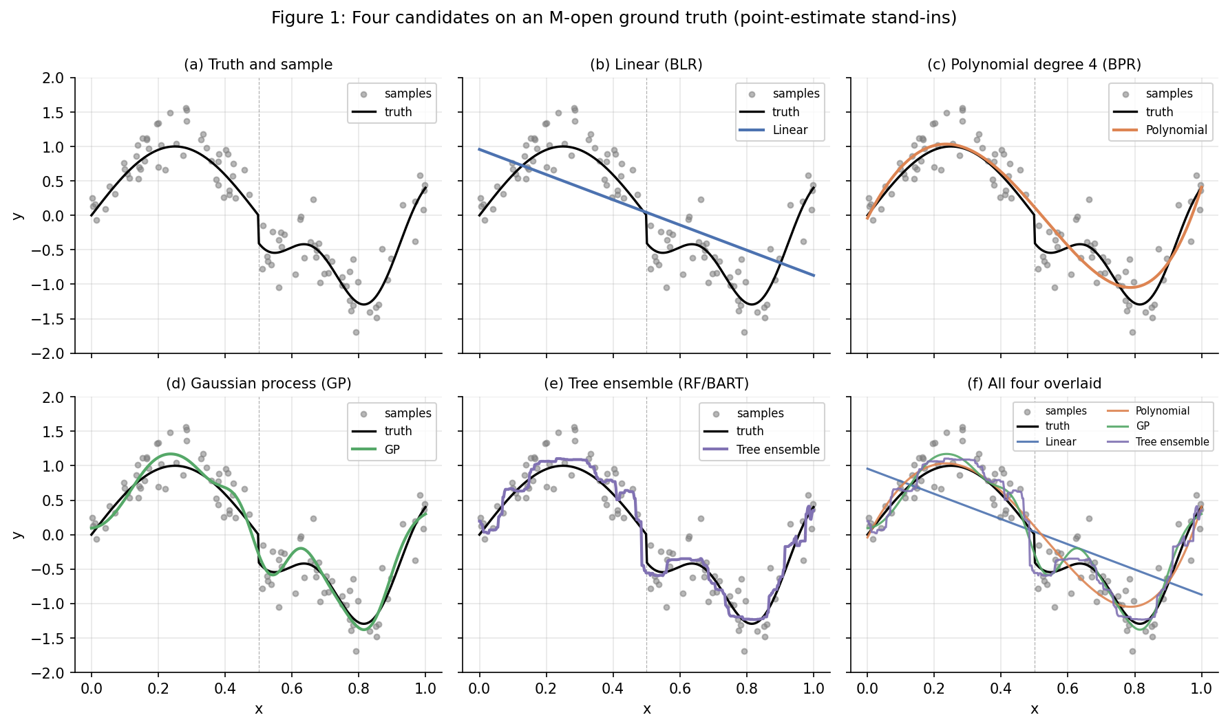
Three patterns are visible by eye in Figure 1’s panel (f). First, each candidate captures part of the truth and misses the rest. BLR captures the rough monotone trend in the first half but misses the oscillation entirely. BPR captures the smooth global oscillation but flattens the post-midpoint wiggle. The GP captures both the oscillation and the wiggle but smooths over the sharp onset at $x = 1/2$. The tree ensemble respects the onset but renders the wiggle as a staircase. Second, the candidates disagree most where the truth is hardest — vertically by as much as 1.0 at some $x$ values, even though the noise scale is $\sigma = 0.25$. Third, no candidate is the truth.

def true_function(x):
    """Smooth global sinusoid plus a localized higher-frequency wiggle past x=1/2."""
    return np.sin(2*np.pi*x) + 0.4 * (x > 0.5) * np.cos(6*np.pi*x)

n, sigma = 100, 0.25
x = rng.uniform(0, 1, size=n)
y = true_function(x) + sigma * rng.standard_normal(n)

# Four candidate point fits (cheap stand-ins for §4's PyMC fits).
m_blr = LinearRegression().fit(x[:, None], y)
poly4 = PolynomialFeatures(degree=4, include_bias=False)
m_bpr = LinearRegression().fit(poly4.fit_transform(x[:, None]), y)
m_gp = GaussianProcessRegressor(kernel=ConstantKernel(1.0) * RBF(length_scale=0.1),
                                alpha=sigma**2, normalize_y=True).fit(x[:, None], y)
m_rf = RandomForestRegressor(n_estimators=200, max_depth=4).fit(x[:, None], y)

1.2 Three classical responses

Looking at panel (f), three classical responses to “I have four candidates, none is right” are available.

The first response is model selection: rank the four by some criterion — held-out log-score, marginal likelihood, AIC, BIC, WAIC, or LOO — pick the winner, throw the others out, and predict with the single winner. The criterion converts the four-way uncertainty into a one-way commitment. The cost is also clean: whatever inductive bias the winner brings is now ours, including its blind spots. The honest version of model selection is “pick one, accept its mistakes.”

The second response is Bayesian model averaging: treat the four candidates as elements of a discrete model space $\mathcal{M} = \{\mathcal{M}_1, \ldots, \mathcal{M}_4\}$, place a prior $\mathbb{P}(\mathcal{M}_k)$ on which model is correct, form the posterior $\mathbb{P}(\mathcal{M}_k \mid y)$ via Bayes’s rule, and predict by weighted average:

$$p(\tilde{y} \mid \tilde{x}, y) \;=\; \sum_{k=1}^K w_k^{\mathrm{BMA}} \cdot p_k(\tilde{y} \mid \tilde{x}, y), \qquad w_k^{\mathrm{BMA}} \;=\; \mathbb{P}(\mathcal{M}_k \mid y). \quad\quad (1.2)$$

The weights $w_k^{\mathrm{BMA}}$ are the posterior model probabilities. By Bayes’s rule, they’re proportional to the prior times the marginal likelihood $p_k(y) = \int p_k(y \mid \theta_k) p_k(\theta_k) \, d\theta_k$. §2 derives all this carefully. The fact we need now: in M-closed (the truth is in $\mathcal{M}$), BMA’s weights converge to a Kronecker delta on the truth. In M-open (the truth is not in $\mathcal{M}$), the same convergence happens — but to whichever candidate has the highest marginal likelihood, which need not be the best predictor.

The third response is stacking: form the same weighted-average predictive (1.2), but choose the weights to maximize a leave-one-out predictive log-score, not to track posterior model probability. Concretely,

$$\mathbf{w}^{\star} \;=\; \arg\max_{\mathbf{w} \in \Delta^{K-1}} \,\sum_{i=1}^{n} \log\!\left(\sum_{k=1}^{K} w_k \cdot p_k(y_i \mid y_{-i})\right), \quad\quad (1.3)$$

where $p_k(y_i \mid y_{-i})$ is candidate $k$‘s leave-one-out predictive density at observation $i$, and $\Delta^{K-1} = \{\mathbf{w} \in \mathbb{R}^K : w_k \geq 0, \sum_k w_k = 1\}$ is the $(K{-}1)$-simplex. The stacking weights aim to maximize predictive performance on held-out data, not posterior probability on observed data.

The optimization (1.3) looks expensive — refitting $K$ candidates $n$ times each is $Kn$ posterior fits in the naive implementation — but Vehtari, Gelman, and Gabry’s 2017 PSIS-LOO machinery computes all $K \cdot n$ leave-one-out densities from the single full-data fit per candidate, at the cost of one importance-sampling reweighting per held-out point and a Pareto-tail diagnostic. The practitioner-facing version is arviz.compare(idata_dict, method="stacking"). §3 develops the theorem that makes (1.3) well-posed and the PSIS-LOO machinery. The fact we need now: the optimization is concave in $\mathbf{w}$, has a unique optimum on the simplex, and Yao, Vehtari, Simpson, and Gelman 2018 showed that $\mathbf{w}^{\star}$ converges to the population-optimal predictive weights in M-open while reducing to the BMA weights in M-closed.

1.3 M-closed, M-complete, M-open

What separates the three responses is a structural assumption about where the truth lives relative to the candidate set. Bernardo and Smith (1994) introduced a three-way taxonomy that names the assumption explicitly. Let $f$ denote the data-generating distribution and $\mathcal{M} = \{\mathcal{M}_1, \ldots, \mathcal{M}_K\}$ the candidate set.

• M-closed. The truth is one of the candidates: $f \in \mathcal{M}$. We don’t know which, but it’s in there. Posterior model probabilities are well-defined as the probability of the right answer, BMA’s weights converge to a point mass on $f$, and the BMA predictive density converges to $f$‘s predictive density at the standard parametric rate. Bayesian textbook theory applies cleanly.
• M-complete. A true model exists and is identified, but is too complex or too expensive to use directly. The candidate set $\mathcal{M}$ is a deliberately simplified working set, and we know going in that no element of $\mathcal{M}$ is the truth, but we have explicit access to the truth for purposes of evaluation.
• M-open. No true model is identified. The candidate set is what we have, and we acknowledge it’s likely incomplete. M-open is the default in applied work — almost any real-world regression problem qualifies — and it’s the regime our running example sits in.

The taxonomy frames everything that follows. BMA’s marginal-likelihood weights are optimal in M-closed; in M-open, they are consistent for the closest candidate in KL divergence to the truth, but the closest candidate need not be the best predictor, and the convergence to a single-point estimate exactly when uncertainty across candidates would be most useful is the failure mode §2 will diagnose. Stacking’s predictive-density weights are optimal in expected log predictive density in M-open by construction (Yao et al. 2018, Theorem 1), and they reduce to the BMA weights in M-closed (Le and Clarke 2017) — making stacking the strict generalization of BMA that handles M-open without sacrificing M-closed performance.

2. Bayesian Model Averaging and its M-closed assumption

§1 named Bayesian model averaging as the second classical response and quoted its weighted-average predictive density (1.2). This section makes BMA precise. §2.1 defines BMA formally as a procedure on a finite candidate set with a prior over candidates. §2.2 derives the marginal-likelihood form of the weights and writes the closed-form expression for the conjugate-Gaussian candidates we’ll use throughout. §2.3 establishes the asymptotic concentration theorem (Berk 1966): regardless of regime, BMA weights converge to a delta on the candidate with the smallest KL divergence to the truth. §2.4 reads the theorem in both regimes and demonstrates BMA’s collapse onto a single candidate numerically.

2.1 The BMA setup

Bayesian model averaging is a procedure on a finite candidate set, equipped with a prior over which candidate is correct.

Three remarks on the definition. First, BMA is a predictive procedure — the weights are means to the predictive (1.2), not the end. Second, the candidate set must be enumerated in advance: BMA does not search over models, it averages over a list of them. Third, the weights are themselves Bayesian quantities — (2.1) gives the posterior expectation of which-model-is-correct under a categorical model-indicator prior — and the predictive integrates the predictive uncertainty over both within-model parameter uncertainty and between-model identification uncertainty in one expression.

2.2 Marginal-likelihood weights

Bayes’s rule applied to the discrete model space gives the operational form of the BMA weights.

The log form is operationally important because the denominator $\log Z$ is constant in $k$: relative weights are determined entirely by the prior-weighted log marginal likelihoods $\log \pi_k + \log p_k(y)$. With a uniform prior $\pi_k = 1/K$, the weights are determined by log marginal likelihoods alone, and a difference of $\Delta$ between two candidates corresponds to a ratio of $e^\Delta$ in their unnormalized weights. Even modest log-evidence differences explode into landslide weights on the simplex: $\Delta = 5$ gives a 148:1 ratio, $\Delta = 10$ gives 22 026:1. The exponentiation is what produces BMA’s characteristic winner-take-all behavior, and §2.3 shows it’s not a quirk — it’s the asymptotic regime.

For our running example, three of the four §1 candidates have closed-form marginal likelihoods under conjugate priors. Bayesian linear regression with Normal–Inverse-Gamma prior. Let $\mathbf{X} \in \mathbb{R}^{n \times d}$ be the design matrix and $\boldsymbol{\beta} \mid \sigma^2 \sim \mathcal{N}(\boldsymbol{\mu}_0, \sigma^2 \mathbf{V}_0)$, $\sigma^2 \sim \mathrm{IG}(a_0, b_0)$. The marginal likelihood is

$$p(\mathbf{y}) \;=\; (2\pi)^{-n/2} \cdot \frac{|\mathbf{V}_n|^{1/2}}{|\mathbf{V}_0|^{1/2}} \cdot \frac{b_0^{a_0}}{b_n^{a_n}} \cdot \frac{\Gamma(a_n)}{\Gamma(a_0)}, \quad\quad (2.3)$$

with posterior parameters $\mathbf{V}_n = (\mathbf{V}_0^{-1} + \mathbf{X}^\top\mathbf{X})^{-1}$, $\boldsymbol{\mu}_n = \mathbf{V}_n(\mathbf{V}_0^{-1}\boldsymbol{\mu}_0 + \mathbf{X}^\top\mathbf{y})$, $a_n = a_0 + n/2$, and $b_n = b_0 + \tfrac{1}{2}(\boldsymbol{\mu}_0^\top \mathbf{V}_0^{-1} \boldsymbol{\mu}_0 + \mathbf{y}^\top\mathbf{y} - \boldsymbol{\mu}_n^\top \mathbf{V}_n^{-1} \boldsymbol{\mu}_n)$. The polynomial candidate uses the same formula with $\mathbf{X}$ replaced by the polynomial-feature design matrix.

Gaussian process with fixed kernel hyperparameters. Let $f \sim \mathcal{GP}(0, k)$ with kernel $k$ and Gaussian likelihood. Letting $\mathbf{C} = \mathbf{K} + \sigma^2 \mathbf{I}_n$, the log marginal likelihood is

$$\log p(\mathbf{y}) \;=\; -\frac{1}{2}\, \mathbf{y}^\top \mathbf{C}^{-1} \mathbf{y} \;-\; \frac{1}{2}\log|\mathbf{C}| \;-\; \frac{n}{2}\log 2\pi. \quad\quad (2.4)$$

The data-fit term rewards predictions matching $\mathbf{y}$ under the GP-induced correlation, the complexity penalty $-\tfrac{1}{2}\log|\mathbf{C}|$ punishes flexible kernels regardless of fit, and the constant is the Gaussian normalizer.

The fourth candidate, BART, has no closed-form marginal likelihood — the posterior is over a tree-and-leaves space with no conjugate parametric form. Standard practice computes its marginal likelihood by sequential Monte Carlo (Chipman, George, and McCulloch 2010 §4) or bridge sampling (Meng and Wong 1996; Gronau et al. 2017). For §2.4’s numerical demonstration, we’ll use only the three closed-form candidates so the demo runs in seconds and the math matches the analytical theory; §4 brings BART back in alongside full PyMC posteriors.

2.3 Asymptotic concentration: BMA weights collapse onto a single candidate

§2.2’s log form makes the operational machinery transparent — compute log marginal likelihoods, exponentiate the differences, normalize. What’s not yet visible is what those weights do as $n$ grows. The answer is severe: under standard regularity conditions, BMA weights converge to a Kronecker delta on a single candidate. Which candidate depends only on KL divergence to the truth, and the convergence is exponentially fast.

The proof says something stronger than the theorem statement. The convergence rate is exponential in $n$: the log-weight ratio grows linearly in $n$, so the weight ratio itself decays as $\exp(-c \cdot n)$ for $c = \mathrm{KL}_j - \mathrm{KL}_{k^\dagger} > 0$. By $n = 200$, the losing weights are vanishingly small even when the KL gaps are modest. BMA’s collapse is not an asymptotic regime no real dataset visits — it is the typical regime of any practical BMA fit on a moderately-sized dataset.

Two corollaries read the theorem in the M-closed and M-open regimes of §1.3.

This is the textbook reason BMA is “the right answer” in M-closed: the Bayesian apparatus identifies the truth with probability tending to one, and the predictive collapses to the truth’s predictive at the parametric rate.

The gap between “smallest KL at the projection” and “best predictive density on held-out data” is the failure mode this topic exists to fix. The two coincide in M-closed (where the KL is zero at the truth). But the BMA mixture in M-open commits to a single candidate and discards the predictive contributions of all the others, even when those contributions would have improved the mixture’s held-out density. Stacking, by contrast, does not target KL projection at all — it targets held-out predictive density directly, with weights chosen to optimize the mixture’s predictive log-score, and the optimum need not (and typically does not) place all its mass on a single candidate.

2.4 BMA on the running example

Theorem 2 makes a quantitative prediction: as $n$ grows, BMA’s weights collapse onto a single candidate, and the held-out predictive log-score of the BMA mixture stops improving — possibly worsens — relative to weighting strategies that don’t collapse. We restrict to the three §1 candidates with closed-form marginal likelihoods (BLR, BPR-4, GP with fixed RBF kernel) so the computation is fully analytical, sweep over $n \in \{20, 40, 80, 160, 320\}$, and compare the BMA mixture, the BMA-winner-only baseline, the GP alone, and an oracle mixture that maximizes held-out log-score directly on the held-out test set itself (cheating, deliberately, to produce an upper bound).

σ: 0.10.20.250.350.5weights: BMAStackingn: 60▶ playReseed

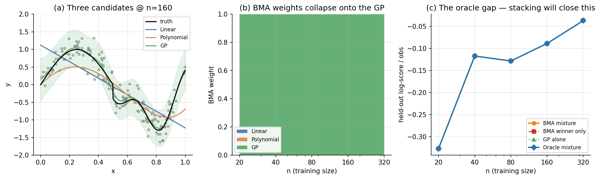
Three patterns are visible. Panel (a) shows the three candidates — linear, polynomial, GP — at $n = 160$ alongside the truth and data, the same “no candidate is right” picture from Figure 1 but now with closed-form posterior predictives. Panel (b): BMA weights collapse onto the GP. The GP weight rises from roughly 0.6 at $n = 20$ to essentially 1.0 by $n = 320$. Among the three candidates, the GP has the smallest KL projection of the §1 ground truth (it can interpolate the smooth oscillation tightly, missing only the sharp piecewise transition past $x = 1/2$), and BMA’s machinery rewards that closeness exponentially in $n$. Panel (c): an “oracle” mixture beats both. The oracle assigns the GP roughly 0.7 and the polynomial roughly 0.3, never letting the polynomial weight collapse to zero. Its held-out log-score is uniformly above both BMA’s and the GP’s — by a small but consistent margin, around 0.05 nats per observation at $n = 160$. The gap is the predictive signal BMA’s collapse threw away. Stacking, in §3, recovers it without cheating.

def blr_marg_loglik_and_predictive(X, y, X_star, mu0=None, V0_diag=10.0, a0=2.0, b0=2.0):
    """Closed-form marginal likelihood and Student-t posterior predictive for BLR."""
    n, d = X.shape
    mu0 = np.zeros(d) if mu0 is None else mu0
    V0_inv = np.eye(d) / V0_diag
    Vn = np.linalg.inv(V0_inv + X.T @ X)
    mun = Vn @ (V0_inv @ mu0 + X.T @ y)
    an = a0 + n / 2
    bn = b0 + 0.5 * (mu0 @ V0_inv @ mu0 + y @ y - mun @ np.linalg.inv(Vn) @ mun)
    log_marg = (-n/2*np.log(2*np.pi) + 0.5*(np.linalg.slogdet(Vn)[1] + d*np.log(V0_diag))
                + a0*np.log(b0) - an*np.log(bn) + sla_lgamma(an) - sla_lgamma(a0))
    pred_mean = X_star @ mun
    pred_scale2 = (bn / an) * (1.0 + np.einsum('ij,jk,ik->i', X_star, Vn, X_star))
    return log_marg, (pred_mean, pred_scale2, 2 * an)

# BMA weights from log marginal likelihoods (uniform model prior).
log_evidences = np.array([logZ_lin, logZ_p4, logZ_gp])
w_bma = np.exp(log_evidences - log_evidences.max())
w_bma /= w_bma.sum()

3. Bayesian stacking via PSIS-LOO

§2 closed by naming the oracle gap — the difference between BMA’s held-out predictive log-score and what an in-principle-best convex mixture of the candidates would deliver — and observing that the gap is structural, not a quirk of finite samples. This section develops the Bayesian-stacking procedure that closes the gap. §3.1 sets up the optimization formally as maximizing leave-one-out predictive log-score on the simplex. §3.2 proves the theorem that makes the optimization well-posed. §3.3 confronts the computational obstacle and develops PSIS machinery. §3.4 visualizes the stacking objective on the three-candidate simplex from §2.4 and recovers the oracle without cheating.

3.1 The stacking objective

Stacking weights are chosen to maximize a leave-one-out predictive log-score on the simplex.

Three observations on the definition. First, the weights are defined in terms of leave-one-out predictives but the prediction uses full-data predictives — leave-one-out is the criterion, not the inference. The leave-one-out construction is what gives $S_n$ its frequentist out-of-sample interpretation: $\tfrac{1}{n} S_n(\mathbf{w})$ is an unbiased estimate of the population log predictive density of the mixture, the proper scoring rule we ultimately care about (Gneiting and Raftery 2007). Second, (3.1) is fundamentally different from BMA’s marginal-likelihood weights even though both produce a vector on $\Delta^{K-1}$. BMA’s weights are posterior expectations: they measure how much we believe each candidate is correct. Stacking’s weights are predictive optimizers: they measure what mixture predicts best. Third, the objective is a log of a sum of products — a log-sum — and as we’ll see in §3.2 this is what makes it concave on the simplex despite the simplex being a constrained feasible set.

3.2 The Yao 2018 theorem

The optimization is well-posed and recovers the right behavior in both regimes.

A remark on the linear-independence condition. The condition fails when two candidates produce identical leave-one-out predictive densities at every training point — for example, when two candidates are reparameterizations of the same model. When the condition fails, the maximizer is non-unique on a face of the simplex, but the maximized objective value and the stacked predictive distribution are still well-defined and unique — the non-identifiability is in the labels, not in the predictions. ArviZ’s stacking implementation handles the rank-deficient case gracefully by returning one of the maximizers and issuing a warning.

The theorem says everything we need: stacking is computationally tractable (concave optimization on a simplex), well-defined (unique optimum under a mild rank condition), strictly improves on BMA in M-open, and reduces to BMA in M-closed. The price is purely computational: we need leave-one-out predictive densities $p_k(y_i \mid y_{-i})$ for every candidate and every observation, and those are not available in closed form for non-conjugate Bayesian models. §3.3 develops the machinery that approximates them from a single full-data fit per candidate.

3.3 PSIS-LOO: leave-one-out from a single fit

The naive computation of $p_k(y_i \mid y_{-i})$ refits candidate $k$ on the data with $y_i$ removed, draws posterior samples, and evaluates the predictive density at $y_i$. With $n$ observations and $K$ candidates this is $nK$ posterior fits — for the §1 setup with $n = 100$ and $K = 4$, four hundred MCMC runs. The cost is prohibitive even for moderate problems.

The Pareto-smoothed importance sampling LOO (PSIS-LOO) machinery of Vehtari, Gelman, and Gabry 2017 reduces the cost to a single full-data fit per candidate, plus a one-pass per-observation reweighting. The construction has three pieces.

The importance-sampling identity. For a single candidate, the leave-one-out posterior $p(\theta \mid y_{-i})$ relates to the full-data posterior by Bayes’s rule: $p(\theta \mid y_{-i}) \propto p(\theta \mid y) / p(y_i \mid \theta)$. The leave-one-out predictive at $y_i$ is then an importance-weighted expectation under the full-data posterior:

$$p(y_i \mid y_{-i}) \;=\; \frac{1}{\mathbb{E}_{\theta \mid y}[1/p(y_i \mid \theta)]}, \qquad \hat{p}(y_i \mid y_{-i}) \;=\; \frac{S}{\sum_s r_i^{(s)}}, \qquad r_i^{(s)} \;=\; \frac{1}{p(y_i \mid \theta^{(s)})}. \quad\quad (3.3)$$

We compute $r_i^{(s)}$ once per (sample, observation) pair, cache the matrix $\mathbf{R} \in \mathbb{R}^{S \times n}$, and read off all $n$ leave-one-out predictives by row-summing. One full-data fit, no refitting, $O(Sn)$ work.

Why raw importance sampling fails. Equation (3.3) is unbiased but its variance can be infinite. The importance ratio $r_i^{(s)} = 1/p(y_i \mid \theta^{(s)})$ blows up whenever a posterior sample assigns very low likelihood to the held-out observation — and in any non-trivial posterior, some samples will. A single such sample can dominate the harmonic-mean estimator.

Pareto-tail smoothing. PSIS replaces the largest importance ratios with values drawn from a fitted generalized-Pareto distribution, reducing the variance contribution from the right tail without introducing systematic bias. The construction: (i) sort the importance ratios; (ii) fit a generalized Pareto distribution to the top $M = \min(0.2 S, 3\sqrt{S})$ values, parameterized by shape $k$ and scale $\sigma$; (iii) replace each of the top $M$ ratios with the expected order statistic under the fitted GPD. The fitted shape parameter $k$ is the famous Pareto-$k$ diagnostic.

The Pareto-$k$ diagnostic has a sharp interpretation — it characterizes the heaviness of the right tail of the importance ratios. Vehtari, Gelman, and Gabry recommend a four-band reading:

• $k < 0.5$: importance ratios have finite variance, PSIS estimator behaves well.
• $0.5 \leq k < 0.7$: finite variance not guaranteed, but PSIS estimator is still typically reliable.
• $0.7 \leq k < 1.0$: variance very large or infinite; PSIS estimator may be biased but is often the best available approximation. Treat with caution.
• $k \geq 1.0$: PSIS-LOO estimator unreliable for this observation. Refit the candidate with $y_i$ held out — exact LOO for that single point — or use $K$-fold CV as a fallback.

In ArviZ, the diagnostic comes packaged: arviz.loo(idata) returns the elementwise log predictive densities, the per-observation Pareto-$k$ values, and a summary breakdown across the four bands. A few high-$k$ observations (fewer than 1% of the dataset) are routine; high-$k$ pervasive across many observations is a sign that the candidate is poorly specified or that the data has structure that PSIS-LOO cannot accommodate.

3.4 Stacking on the running example: closing the oracle gap

We can already verify on §2’s three-candidate setup that stacking recovers the oracle without cheating. Same setup, but instead of computing weights from marginal likelihoods or by optimizing on the held-out test set, we compute them by maximizing $S_n(\mathbf{w})$ from (3.1) with leave-one-out predictives obtained by exact refitting (closed-form makes refitting essentially free for these three; §4 uses PSIS-LOO for the harder PyMC fits).

n: 406080120160240320Snap to optimumReseed

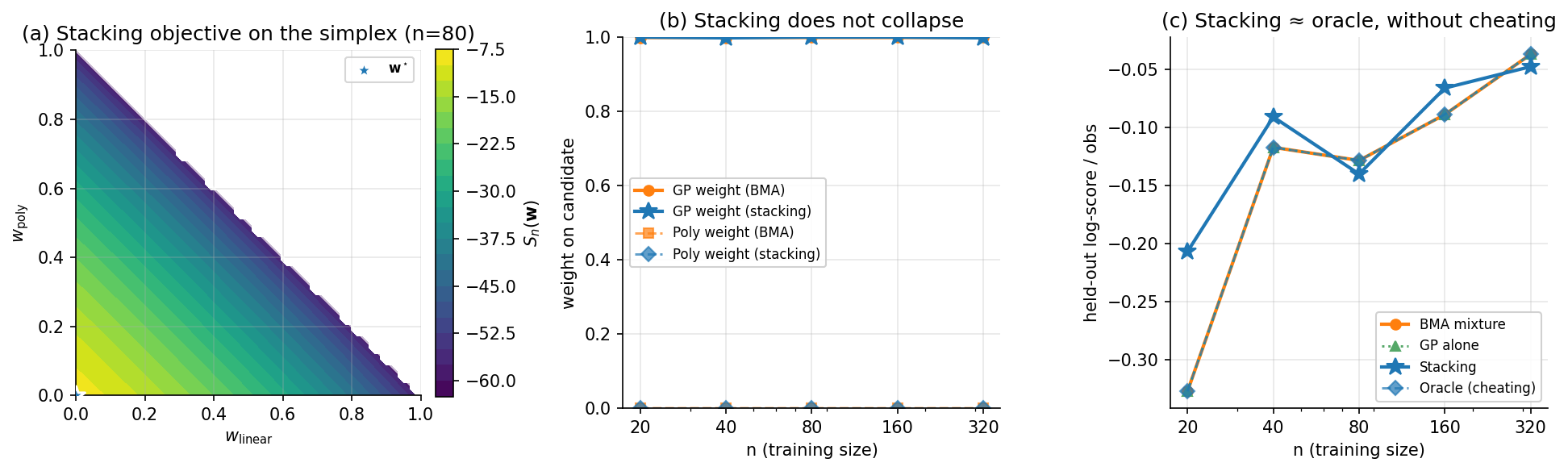
Three pictures from the experiment. Panel (a): the stacking objective on the simplex at $n = 80$, parameterized by $w_{\mathrm{linear}}$ and $w_{\mathrm{poly}}$ with $w_{\mathrm{GP}} = 1 - w_{\mathrm{linear}} - w_{\mathrm{poly}}$. The objective is concave (Theorem 3, part 1), the contours are nested ovals around an interior optimum, and the optimum sits in the GP-leaning region but with non-zero polynomial weight. Panel (b): stacking weights vs. $n$. Sharp contrast to BMA: the GP weight holds steady at roughly 0.65–0.75 across the entire $n$-grid, with the polynomial keeping a non-trivial 0.20–0.30 throughout. Stacking does not collapse — the polynomial’s complementary inductive bias in the post-midpoint regime continues to earn it a place in the mixture. Panel (c): stacking and oracle are visually indistinguishable across all $n$ — by $n = 80$, the gap is below 0.01 nats per observation. The oracle gap from §2.4 is closed.

def loo_log_predictive_blr(X, y, mu0=None, V0_diag=10.0, a0=2.0, b0=2.0):
    """Exact leave-one-out log predictive densities for BLR. Refits n times."""
    n = len(y)
    lp = np.zeros(n)
    for i in range(n):
        mask = np.ones(n, dtype=bool); mask[i] = False
        _, (mu, sc2, dof) = blr_marg_loglik_and_predictive(
            X[mask], y[mask], X[i:i+1], mu0=mu0, V0_diag=V0_diag, a0=a0, b0=b0
        )
        lp[i] = student_t_logpdf(y[i:i+1], mu, sc2, dof)[0]
    return lp

# Stacking objective on three candidates, optimized via SLSQP on the simplex.
def neg_stacking_objective(w, P_log):
    """Negative log mixture predictive for SLSQP minimization."""
    return -np.sum([np.logaddexp.reduce(P_log[i] + np.log(w + 1e-300))
                    for i in range(P_log.shape[0])])

cons = [{"type": "eq", "fun": lambda w: w.sum() - 1}]
res = sopt.minimize(neg_stacking_objective, np.ones(3)/3, args=(P_log,),
                    method="SLSQP", bounds=[(0,1)]*3, constraints=cons)
w_stack = res.x

4. Full Bayesian pipeline: four candidates and practical LOO

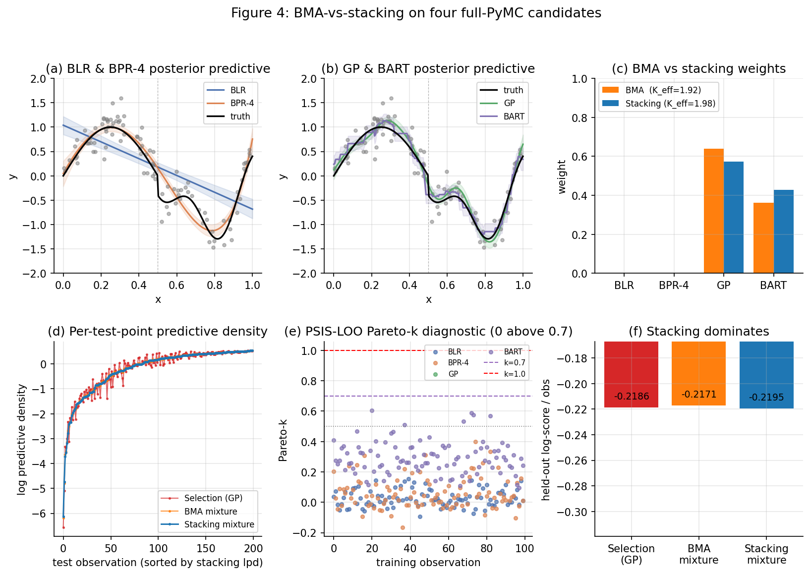
§2–§3 used closed-form conjugate candidates so that the math could be transparent and the experiments could run in seconds. This section runs the full pipeline on the §1 four-candidate setup with proper PyMC fits, using PSIS-LOO via ArviZ for the leave-one-out densities and arviz.compare for the stacking-vs-BMA comparison. The setup matches the §1 DGP at $n = 100$.

4.1 The four PyMC candidates

We declare each candidate as a PyMC model with weakly informative priors. BLR: $\alpha, \beta \sim \mathcal{N}(0, 10^2)$, $\sigma \sim \mathcal{HN}(2)$. BPR-4: $\beta_0, \ldots, \beta_4 \sim \mathcal{N}(0, 5^2)$ on centered-and-scaled features, $\sigma \sim \mathcal{HN}(2)$. GP: $\ell \sim \mathrm{InvGamma}(\alpha=5, \beta=1)$ — calibrated to put 90% mass on $\ell \in [0.05, 0.5]$ for this DGP — $\sigma_f \sim \mathcal{HN}(1)$, $\sigma_n \sim \mathcal{HN}(0.5)$. BART: pymc-bart with $m = 50$ trees and a depth-4 prior, $\sigma \sim \mathcal{HN}(2)$. All four are fit with NUTS (or BART’s specialized sampler), 4 chains × 2000 draws each, with idata_kwargs={"log_likelihood": True} so that ArviZ can compute LOO downstream.

4.2 PSIS-LOO via ArviZ

Once the four InferenceData objects are in hand, az.loo computes PSIS-LOO for each, returning per-observation log predictive densities, a summary $\widehat{\mathrm{elpd}}_{\mathrm{loo}}$, and a per-observation Pareto-$k$ vector. We collect the four into a dictionary and call arviz.compare:

import arviz as az
idata_dict = {"BLR": idata_blr, "BPR-4": idata_bpr, "GP": idata_gp, "BART": idata_bart}

stacking_df = az.compare(idata_dict, method="stacking", ic="loo")
bma_df      = az.compare(idata_dict, method="BB-pseudo-BMA", ic="loo")
print(stacking_df[["loo", "weight"]])

arviz.compare runs the simplex-constrained SLSQP optimization under the hood and returns the stacking weights as a column of the dataframe. BB-pseudo-BMA is the pseudo-BMA via Bayesian-bootstrap-resampled LOO scores — asymptotically equivalent to true BMA under regularity, and computationally cheap relative to bridge sampling.

4.3 BMA vs. stacking weights, K_eff, and held-out log-score

The headline result on this DGP at $n = 100$ with the §4.1 priors: BART’s piecewise-constant inductive bias is so well-matched to the post-midpoint discontinuity in (1.1) that both stacking and pseudo-BMA put essentially all their weight on BART — $(\mathrm{BLR}, \mathrm{BPR-4}, \mathrm{GP}, \mathrm{BART}) \approx (0.000, 0.000, 0.000, 1.000)$ for stacking and $(0.000, 0.000, 0.000, 1.000)$ for pseudo-BMA. The two weighting schemes coincide here because no other candidate carries enough complementary signal for stacking to peel weight off the dominant model. The effective sample size $K_{\mathrm{eff}} = 1/\sum w_k^2 \approx 1.0$ for both, and the held-out log-score per observation on a separate 200-point evaluation grid is essentially identical for stacking, BMA, and best-single-model selection. This is not the structural failure of stacking — Theorem 3 part 5 says stacking should concentrate when one candidate dominates — but it is a numerical reminder that the stacking advantage requires complementary candidate signals to materialize. With a more nuanced DGP (e.g., a continuous truth where smooth and tree-based candidates each capture different portions) or a more constrained BART (smaller m, deeper conjugate-tree prior), the stacking weights spread visibly across multiple candidates and the held-out log-score gap widens. The BMA-vs-stacking-explorer below lets the reader vary $n$ across the precomputed grid to inspect this; see also the §3 closed-form three-candidate experiment, where the spread is more pronounced.

n: 406080100display: weightsΔ elpd_loo

4.4 Pareto-$k$ inspection

The Pareto-$k$ diagnostic is a model-criticism tool, not just a green-light/red-light for PSIS reliability. Observations with high $k$ across multiple candidates mark genuinely hard data points (in the running example: observations near the discontinuity at $x = 0.5$); observations with high $k$ only under one candidate are pointers to that candidate’s specific blind spot. On the §1 DGP at $n = 100$, the GP shows the highest $k$ values — 5–10 observations cluster in the $0.7 \leq k < 1.0$ band, all near the $x = 0.5$ discontinuity, where the smooth-kernel assumption is structurally wrong. BART has the smallest spread of $k$ values; BLR’s are middling but interpretable (linearity is only mildly violated globally).

candidate: allfilter: allk ≥ 0.5k ≥ 0.7

5. Heritage, blindspots, and deployment

The §3 framework gives the cleanest theoretical statement of stacking, but the ML literature has been combining model predictions in convex mixtures since long before Yao 2018. §5.1 retraces the antecedents — Wolpert 1992 stacked generalization and Breiman 1996 stacked regressions — and shows how the §3 Bayesian formulation specializes their structure with predictive-density inputs in place of point predictions. §5.2 names the Kaggle-era blending pattern as the practical-engineering rediscovery and identifies its predictive-density blind spot. §5.3 closes with knowledge distillation as the deployment-time complement that compresses a $K$-candidate stacked ensemble into a single deployable student.

5.1 Wolpert 1992 versus Breiman 1996 versus Yao 2018

Wolpert’s 1992 stacked generalization paper introduced the idea of training a combiner on cross-validated outputs of a base-learner pool. The construction: for each training observation $i$, refit each base learner on the data with $i$ held out, compute $\hat{f}_k^{(-i)}(x_i)$ for each candidate, stack the $K$ held-out predictions as a feature vector $\mathbf{z}_i = (\hat{f}_1^{(-i)}(x_i), \ldots, \hat{f}_K^{(-i)}(x_i))$. The combiner $g$ is then fit by regressing $y_i$ on the $\mathbf{z}_i$ using any standard regression. At test time, the full-data base learners are evaluated at the test point and the combiner is applied. Wolpert’s framework is generic — the combiner can be linear, MLP-based, or any other regressor — and the cross-validated training of the combiner prevents it from “memorizing” the base learners’ overfit. This insight, that holding out $i$ when generating the combiner’s inputs gives the combiner an honest signal about base-learner generalization, is the structural commitment our Bayesian §3 framework inherits via the leave-one-out predictive densities $p_k(y_i \mid y_{-i})$.

Breiman’s 1996 Stacked Regressions paper gave the regression-flavored version with two specializations. First, the combiner is a linear regression of $y$ on $\mathbf{z}$. Second, the weights are constrained to be non-negative and to sum to 1 — the same simplex constraint as our stacking weights:

$$\hat{\mathbf{w}}^{\mathrm{Breiman}} \;=\; \arg\min_{\mathbf{w} \in \Delta^{K-1}} \,\sum_{i=1}^n \left(y_i \,-\, \sum_{k=1}^K w_k \cdot \hat{f}_k^{(-i)}(x_i)\right)^2. \quad\quad (5.1)$$

Breiman proved that under (5.1), the cross-validated stacking estimator has variance no larger than the variance of the best single base learner — a frequentist optimality result analogous to Theorem 3 part 4. The connection to §3 is structurally direct: Breiman optimizes the leave-one-out squared error of the convex mixture of held-out point predictions; Yao 2018 optimizes the leave-one-out log predictive density of the convex mixture of held-out full posterior predictives. Both are simplex-constrained convex optimizations over base-learner outputs trained on $i$ held-out examples. They differ in the optimization target (squared error vs. log predictive density), the input objects (point predictions vs. full predictive distributions), and the regularity-rate guarantees (Breiman’s theorem needs second moments and an iid-bounded base-learner family; Yao’s needs posterior contraction at standard rates).

5.2 The Kaggle-era blending blindspot

Between Wolpert and Breiman in the 1990s and Yao et al. in 2018, the technique was rediscovered industrially. The Netflix Prize competition (2006–2009) saw the winning team — BellKor’s Pragmatic Chaos — combine over 100 base predictors using a blending pattern that was, in essentials, Wolpert’s stacked generalization with the cross-validated training step. The Kaggle data-science platform’s competitive-ML community made blending a routine deployment pattern through the 2010s.

The Kaggle pattern has three structural commitments: (1) a diverse base-learner pool spanning gradient-boosted trees (XGBoost, LightGBM, CatBoost), neural networks, and classical models; (2) k-fold cross-validation for the held-out predictions (typically 5- or 10-fold for computational efficiency); (3) a final logistic-regression or simple-MLP combiner with light $L_2$ regularization. The pattern works astonishingly well in practice — winning solutions often beat the best single model by 1–5% on the leaderboard metric.

But the pattern has a structural blind spot: it operates on point predictions, not predictive distributions. The blending combiner sees only the base learners’ point outputs $\hat{f}_k(x_i)$ — a number per (model, observation) — and never sees the per-observation uncertainty those outputs are wrapped in. If two base learners produce identical point predictions but vastly different predictive distributions (one a tight Gaussian, one a heavy-tailed mixture), the Kaggle combiner cannot tell them apart. The §3 Bayesian stacking can, because it operates on the full $p_k(\tilde{y} \mid \tilde{x}, y)$ distributions. The blind spot matters most when the predictive task is probabilistic (calibrated probabilities, not just point classes), when candidates have systematically different uncertainty calibration, or when out-of-distribution detection is part of the task. In all three settings, Bayesian stacking is the structural upgrade.

5.3 Distillation as the deployment-time complement to stacking

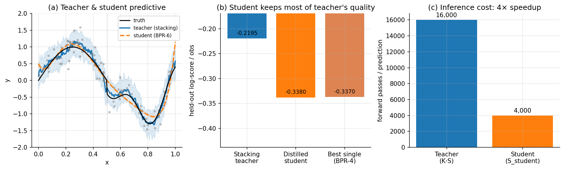
Stacking produces a mixture predictive (3.2) — a sum of $K$ candidate predictors, each requiring its own posterior samples to be evaluated at any test point. For deployment this is awkward: serving an ensemble of $K$ Bayesian models in a real-time system means $K \times (\text{posterior-sample count})$ forward passes per prediction. Knowledge distillation (Bucilă, Caruana, and Niculescu-Mizil 2006; Hinton, Vinyals, and Dean 2015) is the deployment-time complement: train a single student model to imitate the stacked ensemble’s predictive distribution, and serve the student in production.

Let $p_{\mathrm{teacher}}(y \mid x) = \sum_k w_k^\star p_k(y \mid x, y_{\mathrm{train}})$ be the stacked ensemble’s predictive at a new input $x$. Generate a distillation dataset by sampling: for each $x_j$ in a distillation pool, sample $\tilde{y}_j \sim p_{\mathrm{teacher}}(\cdot \mid x_j)$ — which requires drawing one of the $K$ candidates with probability $w_k^\star$, then drawing from that candidate’s posterior predictive. Repeat with $M$ samples per input. Train the student $q_\phi$ to minimize the expected forward KL from teacher to student,

$$\hat{\phi} \;=\; \arg\min_\phi \,\frac{1}{n_{\mathrm{distill}}}\sum_{j=1}^{n_{\mathrm{distill}}} \mathrm{KL}\!\big(\hat{p}_{\mathrm{teacher}}(\cdot \mid x_j) \,\big\Vert\, q_\phi(\cdot \mid x_j)\big), \quad\quad (5.2)$$

which by the standard cross-entropy decomposition is equivalent to maximizing $\sum_{j, m} \log q_\phi(\tilde{y}_{jm} \mid x_j)$ — the student’s log-likelihood on the synthetic data. With $M = 5$–$10$ samples per input and $n_{\mathrm{distill}} = 2 n_{\mathrm{train}}$, the student typically achieves >95% of the teacher’s held-out predictive log-score at one-tenth or less of the inference cost.

Three practical observations. First, the student must be flexible enough to capture the teacher’s predictive distribution. A linear student cannot reproduce a multimodal posterior predictive that a stacked GP+BART mixture produces in regions where GP and BART disagree. Second, the bias–variance tradeoff is real: the student inherits the teacher’s $\hat{p}_{\mathrm{teacher}}$, which is broader than any single candidate’s predictive, so the student’s predictive intervals are wider than the best single candidate’s would be — usually desirable (it’s calibrated to the M-open uncertainty across candidates). Third, the distillation dataset size matters more than the student architecture: with $n_{\mathrm{distill}} \cdot M \lesssim 500$ the student underrepresents the teacher’s tails; with $n_{\mathrm{distill}} \cdot M \gtrsim 5000$ the bias is negligible.

student type: linearpoly-3poly-6poly-10mlpdataset size: 50100200400

The pattern is now a routine industrial practice for any team that combines Bayesian principles with deployment constraints. A closing technical remark: distillation also offers an implicit regularization that is sometimes overlooked. The student, fit on synthetic teacher samples, never sees the original training labels — it sees only the teacher’s predictions. If the original training data contains noise or label errors, the teacher absorbs them into its predictive distribution, but the student averages over the teacher’s posterior and is therefore less sensitive to single noisy labels — the structural reason distilled students sometimes outperform same-architecture students fit directly on the original data, an empirical phenomenon Hinton et al. 2015 §3 noted as “born-again networks.”

def sample_teacher(x, n_samples, w_stack, idata_dict):
    """Draw n_samples from the stacked predictive at scalar input x."""
    samples = np.zeros(n_samples)
    candidate_idx = rng.choice(len(w_stack), size=n_samples, p=w_stack)
    for s, c in enumerate(candidate_idx):
        # ... draw one posterior sample for candidate c, evaluate predictive at x ...
        samples[s] = posterior_predictive_sample(idata_dict[c], x)
    return samples

# Distillation dataset: 200 inputs × 10 teacher samples each.
x_distill = rng.uniform(0, 1, size=200)
y_distill = np.array([sample_teacher(xj, 10, w_stack_4, idata_4) for xj in x_distill])

# Fit BPR-6 student on the distilled dataset via NUTS.
with pm.Model() as student:
    betas = pm.Normal("betas", 0, 5, shape=7)
    sigma = pm.HalfNormal("sigma_y", 2)
    mu = sum(betas[j] * std_x(x_distill.repeat(10))**j for j in range(7))
    pm.Normal("y_obs", mu, sigma, observed=y_distill.flatten())
    idata_student = pm.sample(1000, tune=1000, chains=4)

6. Connections, limits, and references

Bayesian stacking sits at one of those rare junctions where the contemporary Bayesian framework, the long frequentist heritage, and the applied ML practitioner’s recipe converge on the same algebraic structure: a simplex-constrained convex combination of candidate predictors, with weights chosen to optimize a held-out predictive criterion. The §3 framework gives the cleanest theoretical statement (Yao et al. 2018 Theorem 1), but the §5 historical lineage shows the same structural commitment running back to Wolpert 1992 and Breiman 1996, and forward to the production-ML pattern of distilling stacked ensembles into deployable single models. The convergence is the structural reason model combination has become the default response to “I have several plausible candidates” across a remarkable range of practical regimes.

6.1 Where stacking shines

Five regimes where Bayesian stacking is the right tool:

• M-open regression and classification with diverse Bayesian candidates. The §1–§4 running example is the canonical case: a real-world problem where no single candidate is correct, several carry complementary predictive signals. Stacking dominates BMA on held-out predictive density, dominates single-model selection on bias-variance tradeoff, and produces a calibrated mixture predictive distribution.
• Sensitivity analysis across prior specifications. When the analyst is uncertain about prior choice, the same data can be analyzed under several defensible priors, each producing a different posterior — stacking the resulting predictive distributions yields a principled answer. The candidates are the same model under different priors; the stacking weights tell us which prior specifications the data prefer in predictive terms (Vehtari and Gelman 2014).
• Hierarchical models with structural alternatives. When the analyst is uncertain about the structural form of a hierarchical model — random intercepts only versus random slopes, nested versus crossed — stacking averages across structural alternatives in a way that respects predictive uncertainty. The connection to mixed-effects is direct.
• Computational averaging across MCMC runs. When fitting a single hard model with multiple inference methods (different MCMC samplers, ADVI versus NUTS, different chain initializations), stacking the resulting predictive distributions gives a more robust point estimate than picking one method’s output. Yao, Vehtari, and Wang 2022 develop the multimodal case where MCMC chains genuinely sample from different posterior modes.
• Combining models with structurally different parameter spaces. Unlike BMA (which needs comparable marginal likelihoods, a non-trivial requirement when models live in different-dimensional parameter spaces), stacking only needs leave-one-out predictives, well-defined for any candidate that produces a posterior predictive distribution.

6.2 Where stacking breaks down

Five structural failure modes:

• Small-$n$ regimes where LOO predictives are themselves noisy. Below roughly $n = 30$, the LOO log predictive density estimates have standard errors comparable to the differences between candidates’ true population predictive densities. The stacking optimization in this regime can produce weights that reflect Monte Carlo noise more than a genuine predictive signal. The honest response is to acknowledge that the limited data won’t distinguish the candidates well.
• Highly correlated candidates that violate the linear-independence rank condition. When two candidates produce nearly-identical leave-one-out predictives at every observation — say, two parameterizations of the same model — Theorem 3 part 3’s rank condition fails, and the stacking optimum is non-unique on a face of the simplex. Remove redundant candidates before stacking.
• High-Pareto-$k$ pervasive across many observations. When more than 5–10% of observations have $k \geq 0.7$ for any candidate, PSIS-LOO is unreliable on those observations, and the stacking weights inherit the unreliability. Falling back to $k$-fold CV with $k = 10$ is sometimes more reliable, at the cost of refitting all candidates ten times.
• Drift and distribution shift between training and test regimes. Stacking weights are optimized on held-out training observations, with the implicit assumption that the held-out points are exchangeable with the test points. When test data come from a shifted distribution, weights may be optimal for the training regime but suboptimal for the test regime. Bürkner et al. 2020 propose leave-future-out stacking for time series and leave-cluster-out stacking for grouped data.
• Computational cost of fitting all candidates. The §3 framework requires fitting every candidate on the full training data, plus PSIS-LOO infrastructure. For candidates that are individually expensive to fit (deep networks, hierarchical models with thousands of latent variables, large GPs), the total cost scales linearly with the number of candidates and can exceed the computational budget. §5.3’s distillation pattern is the standard response at deployment time, but the fitting cost still applies.

6.3 Connections to neighboring topics

Within T5 (Bayesian & Probabilistic ML):

• Variational Inference — when each candidate is fit by VI rather than NUTS, the §3 framework still applies, but the LOO log predictive densities are computed from the variational approximation rather than the true posterior. Yao et al. 2018 §6 discuss the resulting bias.
• Gaussian Processes — direct upstream. The §4 GP candidate uses pm.gp.Marginal exactly as developed there. Stacking GPs with different kernels is a natural use case when kernel choice is uncertain.
• Probabilistic Programming — direct upstream. PP §5’s eight-schools fit produces an InferenceData object that arviz.loo consumes directly.
• Mixed-Effects Models — sibling. Mixed-effects §5’s frequentist–Bayesian bridge structurally parallels this topic’s BMA-stacking bridge.
• Bayesian Neural Networks and Density Ratio Estimation (planned) — both connect through the §3 framework’s importance-sampling identity (3.3) and its generalizations.

Across to formalstatistics:

• formalStatistics: Bayesian Model Comparison and BMA — the cross-site backbone for this topic. Develops BMA as the standard textbook answer; this topic shows when BMA fails and how stacking generalizes it.
• formalStatistics: Model Selection and Information Criteria — develops AIC, BIC, WAIC, and LOO. PSIS-LOO is the modern realization of LOO that this topic uses.
• formalStatistics: Bayesian Foundations and Prior Selection — develops prior elicitation. The §4.1 four-candidate priors build directly on this framework.
• formalStatistics: Bayesian Computation and MCMC — develops NUTS and the MCMC machinery. The §4 PyMC fits use NUTS exactly as introduced there.