Probabilistic Programming
The PPL abstraction in PyMC, NumPyro, and Stan: trace-based joint log-densities, automatic constrained-to-unconstrained reparameterization, and inference dispatch from NUTS to ADVI to MAP through the eight-schools workflow
Overview
A probabilistic programming language (PPL) is an answer to a structural problem in Bayesian inference: in practice, the modeling step and the inference step have come to be entangled. Running a Gibbs sampler requires full conditionals; running mean-field VI requires deriving the variational updates; running HMC requires the joint log-density and its gradient on unconstrained space. Each of these requires us to do nontrivial calculus on the specific model before we can run the generic algorithm. The PPL move is to cleanly separate the two: the user writes only the generative model, and the language manufactures the joint log-density, the gradients, and the constrained-to-unconstrained reparameterizations the inference engines need.
This topic develops the substrate. §1 motivates the PPL abstraction by computing a Beta–Binomial posterior algebraically and then declaring the same model in PyMC. §2 names the three engine-derived objects (joint log-density, automatic gradient, execution trace) and contrasts PyMC’s PyTensor graph view with NumPyro’s effect-handler trace and Stan’s compiled C++. §3 develops the change-of-variables theorem for the constrained-to-unconstrained transforms HMC needs. §4 dispatches the same generative model to NUTS, ADVI, and MAP and reads the diagnostics. §5 walks the end-to-end Bayesian workflow on Rubin’s eight-schools dataset, including the centered-vs-non-centered reparameterization story. §6 closes with the regimes where PP breaks down and the planned T5 topics that pick up where PP runs out of road.
This is the third topic of T5 Bayesian & Probabilistic ML, after Variational Inference (the projection-based response to intractable posteriors) and Gaussian Processes (the conjugate-with-a-trick response to function-space inference). PP closes the Bayesian-machinery arc by lifting the modeling step into an executable DSL — the same three-line interface that handles the Beta–Binomial in §1 will handle hierarchical models, GLMs, mixture models, and time-series state-space models without per-model derivation work.
1. From explicit Bayes to declarative Bayes
Bayesian inference is a recipe with two parts. We declare a generative model — a prior over parameters and a likelihood that turns parameters into observed data — and then we compute the posterior over the parameters given the data. The first part is modeling: it asks the analyst to commit to assumptions about how the world produced the data. The second part is inference: it’s an integral, , and outside a small list of conjugate pairs it has no closed form.
Probabilistic programming languages are an answer to a structural problem with this recipe: in practice the modeling step and the inference step have come to be entangled. To run a Gibbs sampler we need full conditionals; to run Metropolis–Hastings we need a proposal kernel; to run mean-field VI we need to derive the variational updates. Each of these requires us to do nontrivial calculus on the specific model before we can run the generic algorithm. The PPL move is to cleanly separate the two: the user writes only the model, and the language manufactures the joint log-density, the gradients, and the reparameterizations the inference engines need.
This section makes the move concrete. §1.1 sets up a conjugate Bayesian model — Beta–Binomial — and computes the posterior algebraically, leaning on the prior–likelihood–posterior decomposition from formalStatistics: Bayesian Foundations and Prior Selection . §1.2 declares the same model in PyMC and lets the engine recover the same posterior numerically; the side-by-side comparison is the entire point. §1.3 names the three engine-derived objects that make the recovery possible: the joint log-density, the reparameterization onto unconstrained space, and the execution trace.
1.1 The conjugate playground: Beta–Binomial by hand
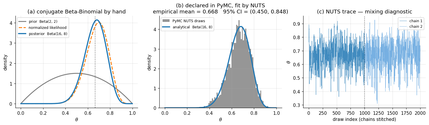
Let be the head probability of a possibly-biased coin. Place a Beta prior on : where is the Beta function and are hyperparameters summarizing prior belief in heads-vs-tails. Flip the coin times independently and observe heads. The likelihood is binomial: Bayes’ rule gives the posterior up to its normalizing constant: where the combinatorial factor and the Beta normalizing constant are absorbed into the proportionality because they don’t depend on . The right-hand side is the kernel of a Beta distribution with parameters , , so the posterior must be exactly that Beta: This is the entire workflow in conjugate-land: prior parameters in, posterior parameters out, no integral computed and no sampler invoked. With , flips, and heads, the posterior is , with mean and a 95% credible interval (computed by inverting the Beta CDF) of approximately .
That this works depends on a happy algebraic accident: the binomial likelihood and the Beta prior have the same functional form in , so when we multiply them the form is preserved. Outside a short list of conjugate pairs — Gaussian–Gaussian, Gamma–Poisson, Dirichlet–multinomial — the denominator integral has no closed form, and direct evaluation of requires either Monte Carlo or optimization.
1.2 The same model, declared
Now we hand the same problem to PyMC. The user-side code is three lines: declare a Beta prior, declare a Binomial likelihood with observed=14 to mark as data rather than a sampled variable, and call pm.sample to run NUTS:
with pm.Model() as model:
    theta = pm.Beta("theta", alpha=2.0, beta=2.0)
    y = pm.Binomial("y", n=20, p=theta, observed=14)
    idata = pm.sample(draws=1000, tune=1000, chains=2)
The histogram of post-warmup posterior draws of should match the analytical density to within Monte Carlo error of order — panel (b) of Figure 1 below is a sanity check that this is what we get.
Notice everything we didn’t do. We didn’t compute the Jacobian of the Beta-to-unconstrained reparameterization NUTS needs. We didn’t differentiate the joint log-density. We didn’t tune the leapfrog step size or the dual-averaging schedule. We didn’t write a Metropolis acceptance ratio. The model spec — three lines — was the entire user-side artifact, and the PPL produced everything else.
For this conjugate problem the PPL is doing more work than the analytical formula needs. The point isn’t that PPLs are necessary here — they aren’t. The point is that the same three-line interface will work when we change the model in ways that destroy conjugacy, and almost any realistic model destroys conjugacy.
1.3 What separates a probabilistic program from a simulator
A simulator is a piece of code that, when run, generates a sample from some distribution. A probabilistic program is a simulator plus three more capabilities, each of which the rest of the topic unpacks:
- Log-density tracing. The engine can run the program and, instead of just emitting samples, emit the joint log-density as a function of the sampled variables. This is what lets us evaluate up to an additive constant for any candidate — the input that NUTS, ADVI, and MAP all need. (Treated in §2.)
- Observation conditioning. The engine can mark some variables as observed — in the example above — at which point it stops sampling them and instead accumulates their log-density into the joint. This is the operational meaning of “conditioning on data”: the program no longer simulates ; it scores how plausible the observed value of is under each candidate parameter. (Also treated in §2.)
- Constrained-to-unconstrained reparameterization. The variable lives on a bounded interval, but HMC/NUTS run on unconstrained . The engine reparameterizes via , computes the Jacobian correction, and presents an unconstrained log-density to the sampler. (Treated in §3.)
These three capabilities — and the fact that the engine derives them automatically from the generative model — are what makes the difference between a Python simulator and a probabilistic program.
2. Anatomy of a probabilistic program
The PPL recovery in §1.2 looked magical — three lines of model spec, no derivations, and out came a posterior. This section unpacks the magic. A probabilistic program produces three engine-derived objects from the generative model: the joint log-density, its automatic gradient, and the execution trace that ties the first two together. Naming these objects and watching how the engine constructs them is the substance of §2.
We work with a slightly larger running example than §1’s Beta–Binomial. Let be real-valued observations and consider the two-parameter model where we have parameterized the likelihood scale by so the latent space is unconstrained — keeping the §3 transform discussion separate from §2’s tracing discussion. §2.1 names the joint log-density and shows how it factorizes over the program’s data-flow graph. §2.2 shows the same density computed two ways: by walking a NumPyro effect-handler trace, and by evaluating a PyMC compiled-graph callable. §2.3 explains observation conditioning as a trace operation. §2.4 closes with Stan’s compiled-C++ contrast — the same abstraction with a different implementation strategy.
2.1 The joint log-density factorizes over the program
A probabilistic program defines a directed acyclic graph (DAG) of named random variables: each sample site introduces a latent variable conditional on its parents, and each observe site introduces an observed variable conditional on its parents. The chain rule for joint distributions on a DAG gives a clean factorization.
Theorem 1 (Joint density factorization).
Let be the random variables encountered during one execution of a probabilistic program in topological order, and let denote the parents of in the program’s data-flow graph. The joint density factorizes as
Proof.
Apply the chain rule for joint densities iteratively in topological order: The DAG structure asserts that is conditionally independent of its non-descendants given . The set , being the predecessors in topological order, contains no descendants of and so is partitioned into and non-descendant non-parents. Conditional independence collapses the second group out of the conditioning set, leaving . The product then matches (2.1).
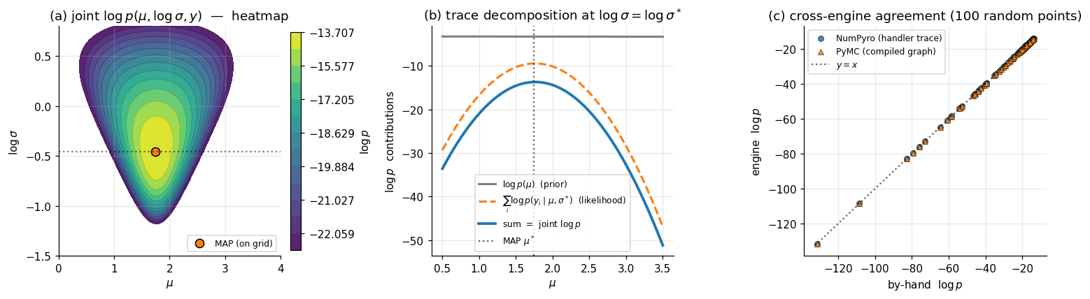
∎For our running model, named sites — , , and (the observation node carrying the full -vector) — with and . The log of (2.1) gives Each summand is a closed-form Normal log-pdf the engine can evaluate from primitive operations; the sum is what the inference engines (NUTS, ADVI, MAP) plug into. Panel (a) of Figure 2 plots this log-density as a heatmap on space; panel (b) decomposes a 1D slice through the heatmap into its prior and likelihood components, exactly as the trace dictionary stores them.
2.2 The trace abstraction: two implementation strategies
The factorization in (2.1) tells us what to compute. Two distinct implementation strategies do the actual computation.
NumPyro: effect-handler trace. At every numpyro.sample("name", dist, ...) call, NumPyro invokes a messenger — a Python context manager — that intercepts the call and dispatches based on which handlers are active. Without any handler, the call samples a value and returns it. With a seed handler, the call uses a deterministic JAX PRNG key. With a condition({"name": value}) handler, the call returns the supplied value rather than sampling. With a trace handler, every sample call is recorded into a dictionary mapping site name to a four-field record: {"type": "sample", "value": ..., "fn": <distribution>, "is_observed": bool}. A single execution of the program under a stack of trace + condition + seed handlers produces a complete record from which the joint log-density follows by accumulating tr[name]["fn"].log_prob(tr[name]["value"]).sum() across all sites. The trace is the operational form of the factorization in (2.1).
PyMC: PyTensor symbolic graph. PyMC takes a different approach. The with pm.Model() as model: context manager builds, behind the scenes, a PyTensor symbolic computation graph whose nodes correspond to the named random variables. At graph-build time, each pm.Distribution("name", ...) call registers a node and a log-prob expression. After the context exits, model.compile_logp() compiles the symbolic graph into a callable Python function that, given a dictionary of parameter values, returns the joint log-density as a single float. The compile step is one-time; the resulting callable runs in C-speed inner loops via PyTensor’s backend (defaulting to NumPy with optional Numba/JAX backends). PyMC’s callable computes (2.1) every time it’s invoked, but the work of deriving the callable from the model spec happens once during compilation.
The two strategies differ in when the program is interpreted — once per execution under handlers (NumPyro), or once at compile time with the resulting graph reused (PyMC) — but both compute the same mathematical object. The cross-engine sanity check in panel (c) of Figure 2 verifies this empirically: at random points in space, the NumPyro-trace log-density and the PyMC-compiled log-density agree to machine precision.
2.3 Observation conditioning is a trace operation
What does observed=y_data actually do? Operationally, it’s a switch on the trace handler: at an observed site, the engine replaces the sampling step with a likelihood-evaluation step. The site still contributes its log-prob to the joint, but the contribution is computed at the supplied data value rather than at a sampled value.
In NumPyro: numpyro.sample("y", dist.Normal(mu, sigma), obs=y_data) is the syntactic marker. At trace time, the messenger sees obs is not None and stores {"type": "sample", "value": y_data, "is_observed": True, ...} in the trace dict. The log-prob accumulator treats observed and unobserved sites identically — both contribute fn.log_prob(value).sum(). The only difference is that the observed value comes from the user, not from a draw.
In PyMC: passing observed=y_data to a distribution constructor flags the variable as data-rather-than-parameter at graph-build time. The compile_logp() callable does not accept the observed variable in its input dict; the observed value is baked into the compiled graph as a constant.
This is the operational meaning of “conditioning on data” in the context of PPLs: the program, run in its unconditioned form, would simulate ; under the observation handler, it scores the supplied against the model. Bayes’ rule never appears explicitly in the engine code — it falls out of (2.2) once we identify the latent variables (whose values vary as we explore the posterior) and the observed variables (whose values are fixed at the data).
2.4 Stan’s compiled-C++ contrast
Stan takes the PyMC strategy further: rather than compiling a Python-callable graph, it compiles the model to standalone C++. A Stan program is a text file in Stan’s domain-specific syntax, with data, parameters, and model blocks declaring the observed inputs, the latent variables, and the joint log-density (via target += ... accumulator statements):
data {
  int<lower=1> N;
  vector[N] y;
}
parameters {
  real mu;
  real log_sigma;
}
model {
  mu ~ normal(0, 10);
  log_sigma ~ normal(0, 1);
  y ~ normal(mu, exp(log_sigma));
}
The Stan transpiler reads the model block, generates C++ source that computes the joint log-density and its gradient via reverse-mode automatic differentiation (Stan’s templated var type), and compiles the C++ to a binary. The binary exposes a log-density-and-gradient function that NUTS, ADVI, and L-BFGS all call. Stan’s compile step is heavier than PyMC’s — a full C++ compilation versus PyTensor’s lighter graph compilation — which is why we don’t run live Stan models in this notebook; the compile time alone exceeds our 60-second budget.
The three implementations — NumPyro’s runtime handler trace, PyMC’s PyTensor symbolic graph, Stan’s compiled C++ — produce the same mathematical object: an evaluable joint log-density with an automatic gradient. The choice between them is engineering, not mathematics. NumPyro’s handler approach makes program semantics explicit and supports complex control flow (recursion, dynamic shapes) most naturally. PyMC’s graph approach gives intermediate compile cost with good interactive iteration. Stan’s compiled approach is the most performant per evaluation and the most rigid about model structure. In §4 we’ll dispatch the same model to PyMC’s NUTS and to NumPyro’s NUTS and watch the same posterior emerge from both.
3. Constrained-to-unconstrained transforms
The three engine-derived objects of §2 — joint log-density, gradient, execution trace — are enough to run gradient-based inference if the latent variables already live in unconstrained . They don’t, in general. A Beta variable lives in . A scale parameter lives in . A correlation matrix lives in a positive-definite cone. A simplex variable lives on the standard simplex. None of these admit unconstrained gradient steps without leaving the constraint set.
The PPL fix is automatic reparameterization: every constrained random variable is silently mapped via a smooth invertible transform to an unconstrained space, the change-of-variables formula adjusts the log-density to compensate, and inference runs on the unconstrained representation. The user writes pm.Beta("theta", 2, 2) and the engine works internally with , adding to the log-density to absorb the Jacobian factor.
§3.1 states and proves the change-of-variables theorem for densities — the single result that makes the entire mechanism work. §3.2 walks through the three transforms PPLs use most often: positive-real via the log transform, bounded interval via logit, and simplex via stick-breaking. The first two get full Jacobian computations; the third is large enough that we state the result and reference the standard derivation. §3.3 explains why HMC needs unconstrained representation operationally and shows how PyMC, NumPyro, and Stan implement the transform table.
3.1 The change-of-variables theorem
Theorem 2 (Change of variables for densities).
Let be a random variable on with density (with respect to Lebesgue measure on ). Let be a smooth bijection with smooth inverse , and let . Then has density where is the Jacobian matrix of at . Equivalently,
Proof.
For any measurable set in the image of , Apply the multivariable change of variables for integrals: substitute , so that : Since this holds for every measurable in the image of , we identify the integrand as the density of : The second equality in the theorem statement follows from the chain-rule identity (with ), so . Taking logs gives (3.1).
∎The two equivalent forms in (3.1) appear in different PPL implementations. The "" form is convenient when the engine starts on the unconstrained side and is generating the constrained version (as in the user-side pm.Normal("eta", 0, 1) + deterministic theta = pm.Deterministic("theta", pm.math.sigmoid(eta)) idiom). The "" form is convenient when the engine starts on the constrained side and is generating the unconstrained version automatically — which is what happens for every constrained variable PyMC and NumPyro touch. Both forms are equivalent up to a sign convention on what “the transform” is taken to be.
3.2 Three transforms in the wild
Positive-real via the log transform
For , take and . The Jacobian is scalar: , so , and (3.1) gives The "" — equivalently, "" — is the Jacobian correction.
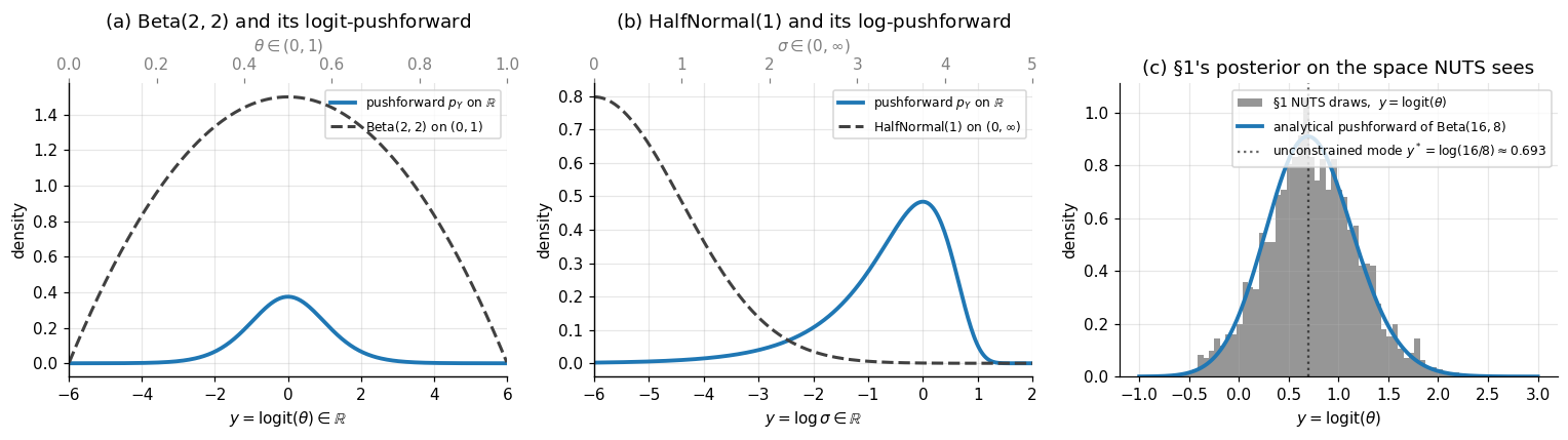
Worked example: half-normal. If with density for , then This density is well-defined on all of . It integrates to 1 — by construction; that’s what the Jacobian factor enforces — and it has tails decaying like for and like for . We verify the unit-integral property numerically in panel (b) of Figure 3 below.
Bounded interval via the logit transform
For , take and . The derivative of the inverse is so , and (3.1) gives The "" is the Jacobian correction.
Worked example: Beta. If with density , the unconstrained log-density is using . The pushforward (3.2) is a smooth bell-curve on for any . Its mode is at — found by setting the derivative of (3.2) to zero, which gives , i.e., . Notice that this differs from the mode of on the constrained space, which is (the standard mode of a Beta density). The two modes are not related by : in general. This is a feature of nonlinear reparameterization — modes are not reparameterization-invariant. (Posterior means are also not reparameterization-invariant: unless is affine.)
Panel (c) of Figure 3 verifies (3.2) by histogramming the §1 NUTS draws of on the logit-transformed scale and overlaying the analytical pushforward density. The agreement is the operational confirmation that PyMC’s NUTS — which sampled the unconstrained representation under the hood — produced draws whose constrained-side post-image matches the analytical conjugate posterior.
Simplex via stick-breaking
For , the standard PPL transform is Stan’s stick-breaking parameterization. Map to by where the shift centers the transform at the simplex centroid (i.e., at , the corresponding ). The Jacobian is lower-triangular, with diagonal entries so its determinant is the product of these diagonals. The full derivation appears in Stan’s Reference Manual (Stan Development Team 2024, §10.7); we use the result operationally without reproving it.
The simplex transform shows that the engine’s transform table is not always a one-line affair — for the simplex, Jacobian terms get added to the log-density. PyMC’s simplex_transform, NumPyro’s StickBreakingTransform, and Stan’s simplex declaration all implement essentially the same mapping under the hood.
3.3 What the engine does, and why HMC needs it
HMC and NUTS simulate Hamiltonian dynamics in the parameter space, taking discrete leapfrog steps that mix gradient evaluations of the log-density with momentum updates. Two operational facts make unconstrained representation essential:
-
Boundary crossings break the dynamics. A leapfrog step from with positive momentum can land at , outside the support of a Beta. The log-density is undefined there, the gradient is undefined, and the proposal is either rejected outright or — worse — produces a NaN that poisons the chain. Reparameterizing to moves the boundary to infinity and removes this failure mode entirely.
-
The unconstrained Hessian sets the step size. NUTS’s dual-averaging step-size adaptation tunes a single scalar to match the local curvature of the log-density. On constrained spaces, that curvature spikes near the boundary — a has finite log-density derivative in the interior but its derivative diverges at or . The unconstrained representation flattens these spikes (the Jacobian terms cancel the boundary singularities), giving a smoother target that adaptive HMC can tune to a single .
The PPL implementation is a transform table indexed by distribution support:
- PyMC registers a
default_transformper distribution class:Intervalfor Beta and Uniform,LogTransformfor HalfNormal and Gamma,LogOddsTransformfor Bernoulli probabilities,SimplexTransformfor Dirichlet,CholeskyCovTransformfor LKJ. The transform is applied automatically; users override withtransform=Noneif they want to supply their own. - NumPyro dispatches via the distribution’s
supportattribute:dist.constraints.unit_intervaltriggersSigmoidTransform,dist.constraints.positivetriggersExpTransform,dist.constraints.simplextriggersStickBreakingTransform, and so on. - Stan uses static type declarations:
real<lower=0>triggers thelogtransform,real<lower=0, upper=1>triggerslogit,simplex[K]triggers stick-breaking,cov_matrix[K]triggers Cholesky-LKJ. The transforms are baked into the generated C++ at compile time.
In all three, the user writes a model on constrained space, and the engine’s NUTS / ADVI / MAP / Pathfinder runs on the unconstrained representation with the Jacobian-corrected log-density. The user never sees the unconstrained variables unless they explicitly ask for them — idata.posterior contains constrained samples, and the unconstrained sister-arrays (e.g., theta_interval__) are stripped from the user-facing output by default.
4. Inference dispatch: NUTS, ADVI, and MAP
The previous three sections built the substrate — the program-as-density abstraction, the trace machinery, the constrained-to-unconstrained transforms — that lets a PPL evaluate and at any candidate . With those primitives in hand, any gradient-based inference algorithm can run on any model the user writes. This section makes the dispatch claim concrete: take a single Bayesian logistic regression model on Iris and fit it three different ways without changing the model spec.
The three engines are NUTS (the No-U-Turn Sampler — exact MCMC up to discretization error), ADVI (Automatic Differentiation Variational Inference — mean-field Gaussian variational approximation), and MAP (maximum a posteriori — point estimate at the mode). NUTS gives the gold-standard posterior at the highest cost; ADVI gives an approximate posterior at intermediate cost; MAP gives a single point at minimal cost. The three exist on a Pareto front of fidelity vs. compute, and the PPL exposes all three from the same model declaration.
We treat each method’s internal mechanics lightly here. NUTS’s convergence theory and detailed-balance proofs live in formalStatistics: Bayesian Computation and MCMC ; ADVI’s ELBO derivation and the reparameterization gradient live in Variational Inference. What we focus on here is the PPL-level observation that none of those internals matter for the user: the same pm.fit(method="advi") and pm.sample() calls work for any model.
§4.1 sets up the running example: Bayesian logistic regression on the Iris versicolor-vs-virginica subset, using petal length and petal width as features. §4.2 walks through NUTS operationally — what no-U-turn means, what dual-averaging does, what divergent transitions signal. §4.3 does the same for ADVI: mean-field Gaussian family, ELBO objective, reparameterization gradient. §4.4 covers MAP via L-BFGS optimization. §4.5 fits the model three times and reads off the diagnostics.
4.1 The running example: Bayesian logistic regression on Iris
Iris (Fisher 1936) is a 150-row dataset with three plant species and four measurements per plant. We restrict to the versicolor-vs-virginica binary subset (classes 1 and 2; 100 rows total) and use the two most discriminative features: petal length and petal width. Both are continuous and roughly Gaussian within each class. The classes overlap mildly — versicolor’s largest petals are smaller than virginica’s smallest — making this a non-trivial but tractable classification problem.
The Bayesian logistic regression model declares an intercept , two slope coefficients , and a Bernoulli likelihood: where is the logistic function (which doubles as the logit-inverse from §3) and is the standardized feature vector for example . Standardizing the features (zero mean, unit standard deviation) puts the slope coefficients on a comparable scale and makes the prior appropriately diffuse.
The latent space is 3-dimensional and unconstrained — none of have constraints, so §3’s transform machinery doesn’t activate. This keeps the dispatch comparison clean: any difference between the three methods comes from the inference algorithm, not from the constraint handling.
4.2 NUTS in 30 seconds
The No-U-Turn Sampler (Hoffman & Gelman 2014) is the dominant default sampler in modern PPLs. It generates posterior samples via Hamiltonian Monte Carlo (HMC), simulating Hamiltonian dynamics with the negative log-density playing the role of potential energy; the gradient from §2 is exactly the force field. HMC produces highly uncorrelated samples by following long trajectories that traverse the posterior efficiently — but vanilla HMC requires two hyperparameters: a leapfrog step size and a trajectory length . NUTS’s “no-U-turn” innovation is to choose adaptively: at each iteration, it doubles the trajectory length until the trajectory makes a U-turn (the position vector and the momentum vector point in opposing directions), then samples uniformly from the trajectory. Dual-averaging step-size adaptation tunes during a warmup phase to hit a target acceptance rate (default 0.8 in PyMC, 0.95 in Stan).
Two diagnostics matter for NUTS:
- Potential-scale-reduction factor measures inter-chain agreement. We run multiple chains from different starting points and compare the variance of within-chain means to the variance of the pooled samples; as chains converge to the same distribution. PyMC and ArviZ flag as concerning. Companion: effective sample size (ESS), which counts how many uncorrelated draws the chain is worth — a small ESS means high autocorrelation and unreliable Monte Carlo estimates.
- Divergent transitions. Discrete leapfrog steps approximate continuous Hamiltonian dynamics; in regions of high curvature (the funnel region of a hierarchical model, for example), the leapfrog approximation breaks down and the integrator’s energy diverges. PyMC counts these “divergent transitions” and reports them. Even a handful of divergences () signals that the posterior has geometry NUTS is struggling to traverse, and the user should investigate before trusting the output.
The full convergence theory — when does HMC converge, at what rate, on what classes of distributions — is the subject of formalStatistics: Bayesian Computation and MCMC . Here we just call pm.sample(...) and read the diagnostics off the resulting idata.
4.3 ADVI in 30 seconds
Automatic Differentiation Variational Inference (Kucukelbir et al. 2017) is the variational engine that ships with every modern PPL. It does three things mechanically:
- Reparameterize. Map the constrained latent variables onto unconstrained using §3’s transform table.
- Posit a mean-field Gaussian variational family. Approximate the posterior on unconstrained space by , parameterized by a mean and log-standard-deviation per dimension.
- Optimize the ELBO via stochastic-gradient ascent with the reparameterization trick. At each step, draw , evaluate the ELBO via Monte Carlo, and update along the gradient.
The reparameterization trick — with — moves the randomness outside the gradient, letting reverse-mode autodiff differentiate through the sampling step. This is the same machinery developed in detail in Variational Inference §4.
ADVI is faster than NUTS by a factor that depends on model size and ELBO convergence speed — typically 5–50× for small models, 100–1000× for big ones. Its cost is structural: the mean-field Gaussian family is the simplest possible variational family, and posteriors with strong cross-correlations between parameters or with non-Gaussian shapes (multimodality, heavy tails, funnels) get distorted by it. The ADVI fit and the NUTS fit will agree to within sampling noise on well-behaved unimodal posteriors and disagree visibly on pathological ones.
The ADVI diagnostic is the ELBO trajectory (or, equivalently, the loss trajectory if the optimizer is minimizing ): a stable, monotonically decreasing loss curve that flattens at a plateau is what we want; a still-decreasing curve at the end of training is a signal to keep going.
4.4 MAP in 30 seconds
The maximum a posteriori (MAP) estimate is the mode of the posterior:
In a PPL, MAP reduces to a single call to a numerical optimizer (PyMC defaults to L-BFGS) that maximizes the same compile_logp callable from §2. There’s no sampling, no variational family, no warmup — just a deterministic optimization that returns a single point.
MAP is fast. It’s also lossy: the entire posterior is collapsed to a point, with no uncertainty estimate. For Gaussian posteriors the MAP is the mean (which is also the mode); for asymmetric posteriors it’s the mode but neither the mean nor the median; for multimodal posteriors it’s whichever mode the optimizer happened to land in. MAP is what classical penalized-likelihood methods compute when you write LogisticRegression(C=...) in scikit-learn — the penalty is a Gaussian prior in disguise, and the regularized solution is the MAP estimate. The PPL gives MAP as a sanity-check option and as a fast initial point for the more expensive methods.
4.5 The dispatch comparison
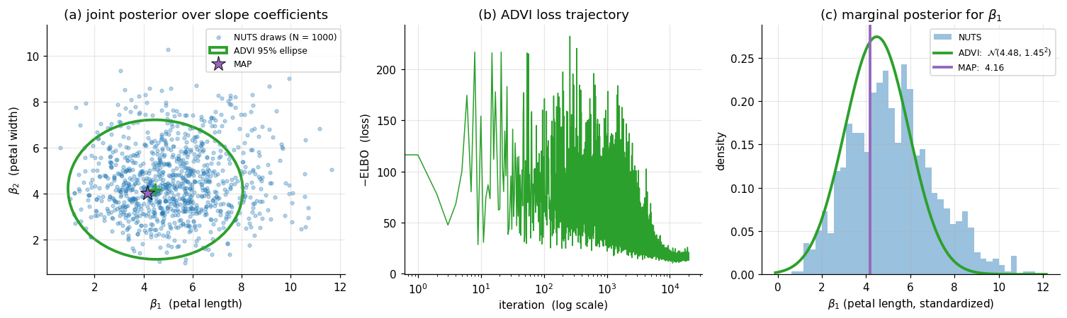
The same model declared in §4.1 is fitted three ways. Figure 4 below shows: (a) the joint posterior over — NUTS draws as a scatter, ADVI’s mean-field Gaussian as a 95%-credible ellipse, MAP as a single star; (b) the ADVI loss trajectory across optimization iterations, showing convergence; (c) the marginal posterior for from each method.
For this problem (a tractable 3-parameter logistic regression with 100 well-separated rows), the three methods agree closely. NUTS converges with and zero divergences. ADVI’s mean-field marginals are slightly tighter than NUTS’s — mean-field underestimates marginal variance when parameters are correlated, and here the petal-length and petal-width slopes have a mild negative correlation that ADVI’s diagonal covariance ignores — and the ADVI ellipse in panel (a) is conspicuously axis-aligned compared to the tilted NUTS scatter. MAP lies essentially at the NUTS posterior mean. The agreement is not coincidence: Iris with continuous features and a moderately informative prior produces a near-Gaussian posterior, exactly the regime where all three methods converge to the same answer at very different costs.
The pedagogical takeaway is twofold. First, the dispatch works: writing the model once and fitting it three ways gave us three matching answers, with no model-specific derivation. Second, the methods are not interchangeable — they’re a Pareto front. NUTS gives uncertainty quantification and is exact up to discretization; ADVI gives uncertainty quantification but is structurally limited by the variational family; MAP gives no uncertainty quantification but is the cheapest. The right choice depends on what the analysis needs. §5 will encounter a model where the three methods don’t all agree, and the disagreement will tell us something useful about the posterior.
5. The Bayesian workflow on eight schools
The dispatch in §4 worked because the posterior was tame — a near-Gaussian, well-conditioned, single-mode logistic regression. Real models often aren’t tame. Hierarchical models in particular have a notorious geometry: when partial-pooling weakens, the posterior pinches into a funnel whose curvature defeats fixed-step-size HMC. This section walks through the iconic example — Rubin’s (1981) eight-schools dataset — and uses it to demonstrate the full Bayesian workflow that PPLs make accessible: declare the model, run a prior predictive check to verify the prior is sensible, fit by NUTS, diagnose, reparameterize the model when diagnostics flag a problem, refit, and finish with a posterior predictive check.
The reparameterization beat is the substantive content. The “centered vs. non-centered” parameterization story is one of the most-cited PPL workflow lessons, because it’s a case where the user has to know enough about the sampler’s geometry to rewrite the model in an equivalent form NUTS can handle. The two parameterizations define the same joint distribution — they describe the same generative process and produce the same posterior on the user-facing parameters — but they offer NUTS different geometries to traverse. PPLs make the rewrite a one-line code change, which is a non-trivial part of why this workflow lesson is teachable at all.
§5.1 introduces the eight-schools data and the standard hierarchical model, with a prior predictive check that puts the prior on a calibration loop. §5.2 fits the centered parameterization with NUTS and watches divergent transitions cluster in the funnel region. §5.3 rewrites the model in non-centered form — algebraically equivalent, geometrically different — and refits cleanly. §5.4 closes with a posterior predictive check that reads the fitted model back against the observed data.
5.1 The data, the model, and a prior predictive check
Rubin (1981) reported the results of an experimental study of “Scholastic Aptitude Test” coaching at schools. Each school ran a randomized controlled trial of a coaching program; for each school we observe an estimated treatment effect (the difference in mean test-score gains between coached and control students at school ) and the standard error of that estimate, computed from the within-school sample sizes and variability:
| School | A | B | C | D | E | F | G | H |
|---|---|---|---|---|---|---|---|---|
| 28 | 8 | -3 | 7 | -1 | 1 | 18 | 12 | |
| 15 | 10 | 16 | 11 | 9 | 11 | 10 | 18 |
The standard hierarchical model treats each school’s true effect as a draw from a population-level distribution with unknown mean and standard deviation : The likelihood treats as known (from the school-level standard errors). Inference produces a joint posterior over — ten unknowns total. The hyperprior on is the partial-pooling lever: small pools the school-level estimates aggressively toward , large pools weakly. The full Bayesian story behind this pooling is in formalStatistics: Hierarchical Bayes and Partial Pooling .
Prior predictive check. Before running inference, the workflow demands a sanity check on the prior: simulate -vectors from the prior and verify they’re consistent with the kind of data we expect to see. For a coaching study, measures a test-score gain in points. If the prior generates values like , the prior is too diffuse and we should retighten before fitting; if the prior generates values like , the prior is too tight. PyMC’s pm.sample_prior_predictive does this with no extra modeling work — the engine reverses the trace machinery from §2 and generates draws from the prior and the prior predictive .
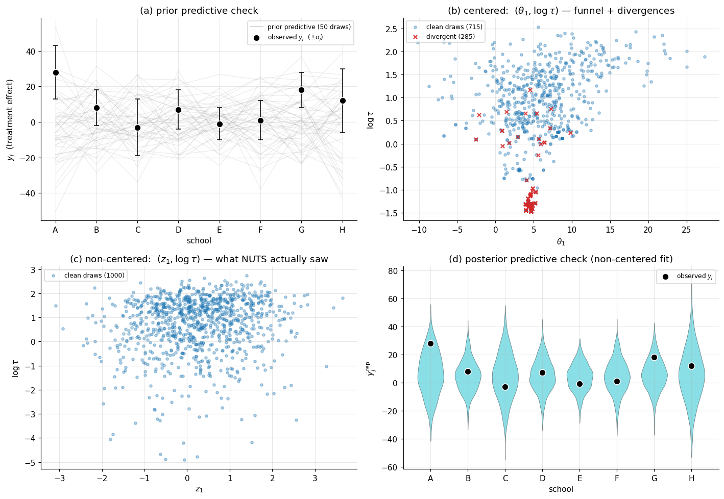
Panel (a) of Figure 5 below overlays 50 prior-predictive draws against the observed vector. The prior generates -values mostly in the range , comfortably containing the observed range . The prior is appropriate without being uninformative — it doesn’t insist on small effects, but it doesn’t license arbitrarily large ones either.
5.2 The centered fit and the funnel
The model spec above is the centered parameterization: each is declared as a draw from , with , , all simultaneously latent. This is the natural way to write the model — it matches the generative story directly. We fit it with NUTS at default settings.
The diagnostics flag trouble. The chain runs and produces samples, but the divergent-transition counter is non-zero — several hundred divergences across 1000 post-warmup draws (the verified notebook reports 285). The for is . The effective sample size for is small, often a few hundred against the nominal 1000 draws. Something is wrong.
The geometric diagnosis is the funnel. The conditional distribution has standard deviation . When is small, is pinched tightly around ; when is large, is loose. As a result, the joint density has a funnel shape: wide at the top ( large), tight at the bottom (). The funnel’s curvature changes rapidly with , and the leapfrog integrator’s fixed step size — even after dual-averaging adaptation — cannot adapt locally. In the wide region, is appropriately tuned; in the narrow region, is far too large, the leapfrog steps overshoot, the integrator’s energy diverges, and PyMC flags a divergent transition.
Panel (b) of Figure 5 plots the centered fit’s draws of as a scatter, with the divergent transitions highlighted in red. The funnel shape is unmistakable: the wide top has dense sampling, the narrow bottom has sparse sampling, and the divergences cluster precisely at the transition between the two — exactly where the integrator’s step size mismatches the local curvature.
The pedagogical point: divergent transitions are not a sampler bug. They’re a signal that the parameterization the user wrote down has a geometry NUTS struggles with. The fix is on the user’s side, not the sampler’s. (Increasing target_accept toward 1 reduces globally, which mitigates divergences at the cost of slower exploration; this is a workaround, not a structural fix.)
5.3 The non-centered reparameterization
The standard fix is the non-centered parameterization. Rather than declare directly, introduce a standard-Normal auxiliary and define as a deterministic transformation of the latents. The user-side code change is three lines:
# centered (struggles with the funnel):
theta = pm.Normal("theta", mu=mu, sigma=tau, shape=J)

# non-centered (clean fit):
z = pm.Normal("z", 0, 1, shape=J)
theta = pm.Deterministic("theta", mu + tau * z)
The two models declare the same joint distribution. To see this, integrate out of the non-centered prior: with implies , exactly the centered prior on . The two models are probabilistically equivalent.
But they are not geometrically equivalent from NUTS’s perspective. In the centered parameterization, NUTS samples jointly, and the joint posterior has the funnel. In the non-centered parameterization, NUTS samples jointly, and under the prior the are independent of . After conditioning on data, the are weakly correlated with — but the joint posterior is a roughly rectangular blob, not a funnel. NUTS traverses it without difficulty.
Panel (c) of Figure 5 plots the non-centered fit’s draws of — the parameter NUTS actually saw — and the contrast with panel (b) is the punchline: the funnel is gone. The post-hoc values reproduce the same marginal posterior on that the centered fit produces (they have to — the models are probabilistically equivalent), but the geometry NUTS navigated to compute that posterior is rectangular rather than funnel-shaped.
The non-centered fit’s diagnostics are clean: zero divergences, for all parameters, full-strength effective sample size. The reparameterization is purely a user-side change to the model code; the engine’s behavior is identical. This is the gift of the PPL abstraction: the rewrite is a 3-line code edit, and the engine’s machinery happily runs on the rewritten model with no further intervention.
5.4 The posterior predictive check
The fit is done. Before trusting it, we run a posterior predictive check (PPC): generate replicated datasets from the posterior predictive distribution and compare them to the observed . If the model is well-specified, the observed should look like a typical draw from . If it doesn’t, the model is mis-specified somewhere, and the prose typically traces the mismatch back to a specific modeling assumption.
PyMC’s pm.sample_posterior_predictive computes the posterior predictive draws by reversing the trace machinery: for each posterior draw of , sample a fresh . The result is a 2D array of shape (chain, draw, school) containing posterior predictive replicates.
Panel (d) of Figure 5 shows the PPC overlay: for each school , the posterior predictive distribution of is shown as a violin (kernel density estimate of the predictive draws), with the observed marked as a single black dot. If the model is well-specified, each black dot lands within the bulk of its corresponding violin. For eight schools, the observed values lie within the bulk of the predictive distributions for all eight — the model is calibrated. School A (with , the largest observed effect) lies further into the right tail of its violin than the other schools, hinting at mild over-shrinkage from partial pooling, but nothing pathological.
A failed PPC tells us about the model. A common pattern: posterior predictive draws are systematically too narrow or too tight, indicating the likelihood doesn’t capture the true data dispersion. Another: the PPC reproduces the marginal mean of but mismatches the tails, indicating that the Gaussian likelihood assumption is incorrect and a heavier-tailed likelihood (Student-) might be more appropriate. The PPC turns “is my model good?” from a vague worry into a specific diagnostic question.
The eight-schools workflow is now complete. We declared a model, ran a prior predictive check (panel a), fit it twice — first in a parameterization NUTS struggled with (panel b), then in an algebraically-equivalent rewrite that NUTS handled cleanly (panel c) — and verified the fit with a posterior predictive check (panel d). The whole loop is the Bayesian workflow the PPL was designed to enable: declarative modeling, multiple inference engines accessible from one model spec, runnable diagnostics at every step, and the freedom to rewrite the model when the diagnostics demand it.
6. Limits, alternatives, and connections
A working PPL is a remarkable artifact: it lifts Bayesian inference from a per-model derivation exercise to a declarative-programming problem. Three lines of model spec and three more for pm.sample produce a posterior. Five lines of model spec and one more for pm.sample_posterior_predictive produce a calibrated predictive distribution. The same three lines of model spec, fed to pm.fit(method="advi") instead of pm.sample, produce an approximate posterior in seconds rather than minutes. The PPL has done what every good abstraction does: it’s let us forget about the implementation while we do the modeling.
It’s not a universal solvent. PPLs work brilliantly on small-to-medium hierarchical models, GLMs, mixture models, time-series state-space models, and most moderately-sized custom Bayesian models — the bread-and-butter of applied Bayesian work. They struggle on large-data regimes, on intractable likelihoods, on high-dimensional latent variables, and on models with discrete latent structure. This section names the regimes where PP shines and the regimes where it doesn’t, and points to the tools that take over when PP runs out of road.
6.1 Where PP shines
The PPL sweet spot is the regime where the user has more domain knowledge to encode than computational resources to spend. Specifically:
- Hierarchical models with up to a few thousand parameters and the partial-pooling structure §5 demonstrated. The eight-schools example scales to thousands of schools without a structural change to the model spec; only the runtime changes.
- Generalized linear models and their Bayesian extensions — logistic, Poisson, multinomial, ordinal, censored, robust. The §4 Iris example was Bayesian logistic regression; swapping to Poisson regression is a one-symbol change.
- Mixture models and latent-class models for clustering and density estimation, where the discrete cluster assignment is marginalized out in the likelihood. PyMC’s and NumPyro’s
pm.Mixture/dist.Mixtureprimitives handle the marginalization automatically. - State-space models — linear-Gaussian, switching, hidden-Markov, autoregressive. Stan is particularly strong here; PyMC’s coverage is improving steadily.
- Bayesian model comparison via predictive performance (LOO-CV, WAIC). ArviZ provides these on top of any PyMC fit.
In all of these, the workflow we walked through in §5 — declare, prior PC, fit, diagnose, refit if needed, posterior PC — runs cleanly with the PPL as substrate.
6.2 Where PP breaks down
Five structural failure modes:
- Large-data regimes. HMC’s gradient evaluation requires a full pass through the data per leapfrog step. For observations, even one HMC iteration takes too long for the sampler to be practical. The standard response is stochastic-gradient MCMC (SG-MCMC) — replace the full-data gradient with a mini-batch estimate, accept the resulting bias, and explore the posterior with a stochastic Langevin or stochastic Hamiltonian dynamic. This is the subject of stochastic-gradient-mcmc.
- Intractable likelihoods. When has no closed form — as in many simulator-based models in epidemiology, ecology, and physics — the engine cannot evaluate the joint log-density and the §2 trace machinery breaks. The standard responses are approximate Bayesian computation (ABC), simulation-based inference (SBI; e.g., neural posterior estimation), and likelihood-free Bayesian methods. None of these fit naturally into a PPL.
- High-dimensional latent variables. When the latent dimension exceeds a few thousand — image-scale models, large neural networks — HMC’s per-iteration cost grows superlinearly and ADVI’s mean-field assumption becomes structurally inadequate. Bayesian neural networks live in this regime; the responses are Laplace approximation at the MAP, MC-dropout as an implicit variational approximation, deep ensembles as a non-Bayesian uncertainty proxy, and Stein variational gradient descent. This is the subject of
bayesian-neural-networks(coming soon). - Discrete latent variables. HMC and ADVI both rely on continuous gradients. Models with discrete latents — variable selection, model averaging, latent-class models that don’t admit closed-form marginalization — require either Gibbs sampling or auxiliary-variable tricks. PyMC’s
pm.NUTSfalls back to Metropolis or Gibbs for discrete variables, but performance degrades. Stan’s response is to require the user to marginalize discrete latents analytically before passing to the sampler. - Multimodal posteriors. HMC can get stuck in a single basin. Tempered transitions, parallel tempering, and sequential Monte Carlo (SMC) are the responses. PyMC has
pm.sample_smcfor this; it runs much slower than NUTS but handles multimodality.
The honest summary: a PPL is great at the workflow we walked through in §§1–5, and it’s not the right tool for at least four well-defined regimes outside that workflow. Knowing when to reach for a PPL — and when to reach for SG-MCMC, ABC, Laplace, or SMC instead — is part of becoming a competent Bayesian modeler.
6.3 Connections to neighboring topics
Within formalML’s T5 Bayesian & Probabilistic ML track:
- Variational Inference is upstream: §4.3’s ADVI relies on the variational-objective and reparameterization-gradient machinery developed there.
- Gaussian Processes is a sibling: the conjugate-Gaussian-likelihood case where closed-form posterior inference is available without a PPL. PyMC and NumPyro both expose GP modules (
pm.gp,numpyro.contrib.gp) that wrap the closed-form expressions in the PPL idiom. - Bayesian Neural Networks (coming soon) is downstream: when latent dimensions get into the thousands and ADVI breaks structurally, the PP workflow needs the heavier machinery developed there.
- Sparse Bayesian Priors is a natural follow-up: horseshoe and regularized-horseshoe priors are notoriously HMC-hostile in their naive parameterizations, and the §5 reparameterization story extends to them. The Sparse Bayesian Priors topic §6 develops the funnel pathology and the Piironen-Vehtari regularization fix in full geometric detail.
- Meta-Learning (coming soon) and Stochastic-Gradient MCMC are responses to the failure modes in §6.2.
Across to formalstatistics:
- formalStatistics: Bayesian Foundations and Prior Selection develops the prior–likelihood–posterior decomposition the PPL automates.
- formalStatistics: Bayesian Computation and MCMC supplies the HMC/NUTS theory PP defers to.
- formalStatistics: Hierarchical Bayes and Partial Pooling develops why partial-pooling models like §5’s eight-schools work, and what the partial-pooling regime gives us over no-pooling and complete-pooling.
PP is the bridge between the Bayesian theory the formalstatistics topics develop and the modern Bayesian-ML applications the rest of the formalML T5 track will build on.
Connections
- §4.3's ADVI dispatch reuses the variational-objective and reparameterization-gradient machinery developed in variational-inference. The mean-field Gaussian family ADVI fits is exactly the family discussed there; the structural cost (axis-aligned ellipses, marginal-variance underestimation under correlation) shows up visibly in §4.5's Iris dispatch comparison. variational-inference
- GPs are the conjugate-Gaussian-likelihood case where closed-form posterior inference is available without a sampler. PyMC and NumPyro both expose GP modules (`pm.gp`, `numpyro.contrib.gp`) that wrap the closed-form expressions in the PPL idiom — the same three-line interface that handles the Beta–Binomial in §1 handles the GP regression posterior on the same footing. gaussian-processes
- §4.3's ADVI minimizes reverse KL between the variational family and the posterior, exactly the projection developed in kl-divergence. Mean-field's mode-seeking pathology — visible as the axis-aligned ADVI ellipse in §4.5 — is one face of reverse-KL's mode-seeking asymmetry. kl-divergence
- ADVI's optimization (stochastic gradient ascent on the ELBO) and MAP's optimization (L-BFGS on the joint log-density) both reduce to the gradient-descent machinery developed there. PP makes the same `compile_logp` callable available to either optimizer without the user touching gradient code. gradient-descent
References & Further Reading
- book Pattern Recognition and Machine Learning — Bishop (2006) Chapters 10 (variational inference) and 11 (sampling methods) supply the algorithmic substrate PP automates (Springer).
- paper The Use of Multiple Measurements in Taxonomic Problems — Fisher (1936) The Iris dataset used in §4's logistic-regression dispatch comparison (Annals of Eugenics).
- book Bayesian Data Analysis — Gelman, Carlin, Stern, Dunson, Vehtari & Rubin (2013) BDA3 — the standard reference for the Bayesian workflow §5 walks through (Chapman and Hall/CRC).
- paper Estimation in Parallel Randomized Experiments — Rubin (1981) The original eight-schools dataset and hierarchical model used in §5 (Journal of Educational Statistics).
- paper A Conceptual Introduction to Hamiltonian Monte Carlo — Betancourt (2017) The standard pedagogical treatment of HMC. §4.2 is a 30-second sketch; this is the long version (arXiv).
- paper Hamiltonian Monte Carlo for Hierarchical Models — Betancourt & Girolami (2015) The centered-vs-non-centered reparameterization paper — the §5 funnel-diagnosis story comes from here (Chapman and Hall/CRC).
- paper Inference from Iterative Simulation Using Multiple Sequences — Gelman & Rubin (1992) The original $\hat{R}$ paper. §4.2's potential-scale-reduction-factor diagnostic is from here (Statistical Science).
- paper The No-U-Turn Sampler: Adaptively Setting Path Lengths in Hamiltonian Monte Carlo — Hoffman & Gelman (2014) The NUTS paper. §4.2's no-U-turn criterion and dual-averaging step-size adaptation are from here (JMLR).
- paper Auto-Encoding Variational Bayes — Kingma & Welling (2014) The reparameterization-trick paper. §4.3's ADVI sketch invokes the gradient estimator developed here (ICLR).
- paper Automatic Differentiation Variational Inference — Kucukelbir, Tran, Ranganath, Gelman & Blei (2017) The ADVI paper. §4.3 is a 30-second sketch of the algorithm developed here (JMLR).
- paper MCMC Using Hamiltonian Dynamics — Neal (2011) The standard book chapter on HMC. §4.2 leans on Neal's exposition (Handbook of Markov Chain Monte Carlo).
- paper A General Framework for the Parametrization of Hierarchical Models — Papaspiliopoulos, Roberts & Sköld (2007) The non-centered parameterization in its general form. §5.3's three-line rewrite is one instance of the framework developed here (Statistical Science).
- paper Rank-Normalization, Folding, and Localization: An Improved $\hat{R}$ for Assessing Convergence of MCMC — Vehtari, Gelman, Simpson, Carpenter & Bürkner (2021) The modern $\hat{R}$ — what ArviZ actually computes. §4.2's diagnostic discussion uses this version (Bayesian Analysis).
- paper Pathfinder: Parallel Quasi-Newton Variational Inference — Zhang, Carpenter, Gelman & Vehtari (2022) Pathfinder — a fast variational alternative competitive with ADVI on well-behaved posteriors (JMLR).
- paper Stan: A Probabilistic Programming Language — Carpenter, Gelman, Hoffman, Lee, Goodrich, Betancourt, Brubaker, Guo, Li & Riddell (2017) The Stan paper. §2.4's compiled-C++ contrast leans on the architecture described here (Journal of Statistical Software).
- paper Composable Effects for Flexible and Accelerated Probabilistic Programming in NumPyro — Phan, Pradhan & Jankowiak (2019) The NumPyro paper. §2.2's effect-handler trace abstraction is exactly NumPyro's design (arXiv).
- paper Probabilistic Programming in Python Using PyMC3 — Salvatier, Wiecki & Fonnesbeck (2016) The PyMC paper. §2.2's PyTensor symbolic-graph approach is what this paper introduced (PeerJ Computer Science).
- book Stan Reference Manual, version 2.34 — Stan Development Team (2024) The Stan transform-table reference. §3.2's stick-breaking simplex transform follows §10.7 here verbatim.