Gaussian Processes

Overview

A Gaussian process is a probability distribution over functions, specified by a mean and a kernel, with the property that every finite collection of function values is jointly multivariate Normal. The function-space view it makes possible — place the prior on the function, not on the parameters — is the canonical Bayesian regression model and the second pillar of the T5 Bayesian & Probabilistic ML track, building on the variational machinery of Variational Inference. Given a kernel, the posterior over function values at any test inputs is a closed-form multivariate Normal computable from kernel evaluations alone, with calibrated uncertainty for free in the conjugate-Gaussian-likelihood case.

This topic develops the substrate. §1 motivates the move from parametric Bayesian regression to function-space priors. §2 fixes the GP definition and verifies that positive-definite kernels yield internally consistent finite-dimensional joints. §3 derives the conjugate-Gaussian regression posterior in closed form via multivariate-Normal conditioning. §4 surveys the kernel zoo and the inductive bias each kernel encodes. §5 turns the kernel hyperparameters from quantities we set by hand into quantities we learn from the marginal likelihood. §6 closes with the $O(n^3)$ Cholesky bottleneck and three structural responses — Nyström, sparse variational GPs, and random Fourier features — plus connections to the rest of formalML and forward-link topics on the T5 roadmap.

1. From parametric Bayes to function-space priors

Bayesian regression starts with a parametric model. Pick a fixed basis $\boldsymbol\phi(\mathbf{x}) = (\phi_1(\mathbf{x}), \ldots, \phi_D(\mathbf{x}))^\top$ — polynomials, splines, RBFs at fixed centers — write the regression function as a linear combination $f(\mathbf{x}) = \mathbf{w}^\top \boldsymbol\phi(\mathbf{x})$, place a Gaussian prior on the weights $\mathbf{w} \in \mathbb{R}^D$, and the posterior is the standard conjugate-Gaussian update from formalStatistics: Bayesian Foundations . The procedure is clean and closed-form. Its weakness is structural: by committing to a fixed $D$-dimensional basis up front, we have committed to a $D$-dimensional family of regression functions, and no amount of data will let $f$ wander outside it.

Gaussian processes lift that commitment. Rather than choosing a basis and a prior over its coefficients, place the prior directly on the function $f$ — a probability distribution over a far richer space — and never name a basis at all. This section makes the move precise. §1.1 unpacks the parametric starting point and observes a fact that motivates everything that follows: parametric Bayesian regression already puts a Gaussian distribution on functions. §1.2 shows what’s wrong with that distribution — its covariance has a built-in low-rank constraint that the basis dimension cannot exceed. §1.3 reads the constraint as a permission slip: skip the basis, choose the covariance directly, and the function-space prior we get is exactly a Gaussian process.

1.1 Bayesian linear regression already puts a Gaussian prior on functions

Let $\mathbf{x} \in \mathcal{X}$ denote an input — we will mostly take $\mathcal{X} = \mathbb{R}$ or $\mathbb{R}^d$ in this topic — and let $\boldsymbol\phi : \mathcal{X} \to \mathbb{R}^D$ be a fixed feature map. Two running examples: the cubic polynomial map $\boldsymbol\phi(x) = (1, x, x^2, x^3)^\top$, and an RBF basis at fixed centers $c_1, \ldots, c_K$ with width $\omega > 0$, $\boldsymbol\phi(x)_k = \exp\!\bigl(-(x - c_k)^2 / (2\omega^2)\bigr)$. The Bayesian linear-regression model is $f(\mathbf{x}) \;=\; \mathbf{w}^\top \boldsymbol\phi(\mathbf{x}), \qquad y_i \;=\; f(\mathbf{x}_i) + \varepsilon_i, \qquad \varepsilon_i \stackrel{\mathrm{iid}}{\sim} \mathcal{N}(0, \sigma_n^2),$ with a Gaussian prior on the coefficients $\mathbf{w} \sim \mathcal{N}(\mathbf{0}, \boldsymbol\Sigma_w)$ and Gaussian observation noise of variance $\sigma_n^2 > 0$. We use $\sigma_n$ for noise throughout the topic and reserve $\sigma_f$ for kernel signal variance once it appears in §2.

The prior on $\mathbf{w}$ induces a prior on $f$. Evaluating $f$ at any single input $\mathbf{x}^*$ gives $f(\mathbf{x}^*) = \mathbf{w}^\top \boldsymbol\phi(\mathbf{x}^*)$, a linear functional of the Gaussian random vector $\mathbf{w}$, so it is itself a Gaussian random variable with mean zero and variance $\boldsymbol\phi(\mathbf{x}^*)^\top \boldsymbol\Sigma_w \boldsymbol\phi(\mathbf{x}^*)$. The same calculation applies jointly to any finite collection of inputs $\mathbf{x}_1^*, \ldots, \mathbf{x}_n^*$: stack the function values into $\mathbf{f}^* = (f(\mathbf{x}_1^*), \ldots, f(\mathbf{x}_n^*))^\top \in \mathbb{R}^n$ and the feature evaluations into $\boldsymbol\Phi^* \in \mathbb{R}^{n \times D}$ with rows $\boldsymbol\phi(\mathbf{x}_i^*)^\top$. Then $\mathbf{f}^* = \boldsymbol\Phi^* \mathbf{w}$, a linear map of the Gaussian $\mathbf{w}$, jointly Gaussian: $\mathbf{f}^* \;\sim\; \mathcal{N}\!\bigl(\mathbf{0},\; \boldsymbol\Phi^* \boldsymbol\Sigma_w (\boldsymbol\Phi^*)^\top\bigr).$ Reading the entries: $\mathbb{E}[f(\mathbf{x})] = 0$ and $\mathrm{Cov}\bigl[f(\mathbf{x}),\, f(\mathbf{x}')\bigr] \;=\; \boldsymbol\phi(\mathbf{x})^\top \boldsymbol\Sigma_w \boldsymbol\phi(\mathbf{x}').$

This is the function-space view of parametric Bayes. The prior on $\mathbf{w}$ — a distribution over a $D$-dimensional weight vector — is equivalent to a particular distribution over functions, characterized by the property that the joint distribution of $(f(\mathbf{x}_1), \ldots, f(\mathbf{x}_n))$ at any finite set of inputs is multivariate Normal with the covariance just displayed. We never had to leave the space of weight vectors to do calculations, but as a pure mathematical object, the prior over $f$ is what the model has put on the table.

1.2 The covariance is finite-rank by construction

The function-space prior we just wrote down has a structural property worth staring at. Define the bivariate function $k_\phi(\mathbf{x}, \mathbf{x}') = \boldsymbol\phi(\mathbf{x})^\top \boldsymbol\Sigma_w \boldsymbol\phi(\mathbf{x}')$. For any finite collection of inputs $\mathbf{x}_1, \ldots, \mathbf{x}_n$, the implied $n \times n$ covariance matrix factors as $\mathbf{K} = \boldsymbol\Phi \boldsymbol\Sigma_w \boldsymbol\Phi^\top$, where $\boldsymbol\Phi \in \mathbb{R}^{n \times D}$ has rows $\boldsymbol\phi(\mathbf{x}_i)^\top$. The rank of a product of matrices is bounded by the rank of any factor, so $\mathrm{rank}(\mathbf{K}) \;\le\; D.$ Whenever we evaluate at $n > D$ inputs, the implied $n$-dimensional Gaussian over $(f(\mathbf{x}_1), \ldots, f(\mathbf{x}_n))$ is degenerate — its support is a $D$-dimensional affine subspace of $\mathbb{R}^n$, and at least $n - D$ of its eigenvalues are exactly zero. The function-space prior knows that all values of $f$ collapse onto a $D$-dimensional surface no matter how many points we look at it from.

This is the structural cost of having committed to a finite basis. In a low-data regime ($n < D$), we won’t notice — the covariance is full-rank on the points we have. In a moderate-data regime ($n \approx D$), the model is right at the edge of capacity and is prone to interpolating noise. In a large-data regime ($n \gg D$), the function class is too small to host the truth, and the posterior concentrates on the closest member of the $D$-dimensional family no matter how badly that member misses. Adding basis functions is the obvious response, but it pushes the choice elsewhere: how many, where centered, of what width. The model designer pays in basis selection what they save in inference.

1.3 The function-space view: place the prior on $f$ directly

Reading §1.1–§1.2 more carefully, we notice something useful. The function-space prior on $f$ is fully characterized — for the purposes of any computation we will ever do — by the bivariate function $k_\phi(\mathbf{x}, \mathbf{x}') = \mathrm{Cov}[f(\mathbf{x}), f(\mathbf{x}')]$ and the mean function $\mu(\mathbf{x}) = \mathbb{E}[f(\mathbf{x})] = 0$. We never store an entire function in memory; we only ever evaluate it at finitely many inputs. So the operational specification of a prior over functions only needs to provide, for any finite collection of inputs, a joint distribution over the function values. The Gaussian-process move drops the feature map.

A Gaussian process is a distribution over functions $f : \mathcal{X} \to \mathbb{R}$ specified by a mean function $\mu : \mathcal{X} \to \mathbb{R}$ and a kernel $k : \mathcal{X} \times \mathcal{X} \to \mathbb{R}$, with the property that for any finite collection of inputs $\mathbf{x}_1, \ldots, \mathbf{x}_n \in \mathcal{X}$, the joint distribution of $(f(\mathbf{x}_1), \ldots, f(\mathbf{x}_n))$ is multivariate Normal with mean vector $\boldsymbol\mu_i = \mu(\mathbf{x}_i)$ and covariance matrix $\mathbf{K}_{ij} = k(\mathbf{x}_i, \mathbf{x}_j)$. We will write $f \sim \mathrm{GP}(\mu, k)$ and (throughout this topic, unless otherwise noted) take $\mu \equiv 0$ for simplicity. The $D$-dimensional basis is gone. The kernel is the only thing we choose.

What changes? Two things, both consequential.

The kernel need not be finite-rank. The kernel $k_\phi$ from a parametric model is bilinear in a $D$-dimensional feature representation, so as a kernel matrix on $n$ inputs its rank is capped at $D$. Many natural kernels — the squared-exponential $k(\mathbf{x}, \mathbf{x}') = \sigma_f^2 \exp\!\bigl(-\|\mathbf{x} - \mathbf{x}'\|^2 / (2\ell^2)\bigr)$, the Matérn family, the periodic kernel — have no such cap. As kernel matrices on $n$ inputs they are generically full-rank, and the function-space prior they induce is correspondingly richer.

Validity now requires an argument. The parametric model gave us the function-space prior for free, because its construction (sample $\mathbf{w}$, plug into $f(\mathbf{x}) = \mathbf{w}^\top \boldsymbol\phi(\mathbf{x})$) builds a single random function whose finite-dimensional marginals automatically agree. The GP construction goes the other way: it specifies the finite-dimensional marginals first and asks whether some random function has them as its marginals. Whether such a function exists, and whether the marginals are mutually consistent — for example, the marginal of the joint over $(f(\mathbf{x}_1), f(\mathbf{x}_2))$ obtained by integrating out $f(\mathbf{x}_2)$ must equal the directly-specified marginal of $f(\mathbf{x}_1)$ — is the content of the Kolmogorov extension theorem. §2 makes this precise and uses it to verify that any positive-definite kernel does in fact define a Gaussian process.

Figure 1 below shows what the move buys us. Reading the columns left to right is the structural lift the rest of this topic exploits.

D (poly): 4K (RBF): 6ℓ (GP): 0.70

Reading left to right is the structural lift §1 develops: the same plot conventions, increasing functional richness. The polynomial family is D-dimensional; the RBF family is K-dimensional; the GP family is infinite-dimensional. Drag the sliders to feel each axis.

The question §2 takes up is what it means, formally, to place a probability distribution on a space of functions in the first place — and which kernels qualify. §3 develops the closed-form posterior given data. §4 surveys the kernels that do most of the practical work. §5 turns the kernel hyperparameters from quantities we set by hand into quantities we learn from the marginal likelihood. §6 closes with the $O(n^3)$ bottleneck that comes free with the construction and three responses to it.

2. Gaussian processes as priors over functions

§1 closed with a definition we have not yet earned: a Gaussian process is a distribution over functions specified by a mean and a kernel, with the property that every finite collection of function values is jointly Gaussian. Two questions are open. Which bivariate functions $k(\mathbf{x}, \mathbf{x}')$ qualify as kernels? And, given a kernel, does an actual probability distribution over functions exist whose finite-dimensional marginals match the prescription? §2.1 fixes the formal definition. §2.2 identifies the answer to both questions — positive-definiteness — and proves that PD kernels yield internally consistent finite-dimensional joints, so by the Kolmogorov extension theorem a Gaussian process exists. §2.3 surveys three canonical kernels with prior-samples pictures, deferring the full design discussion to §4. §2.4 sketches the spectral / Mercer view that justifies §1.3’s “infinite-dimensional” claim.

2.1 The definition

The notation deserves explicit unpacking. The index set $\mathcal{X}$ is whatever space the inputs live in — $\mathbb{R}$ for time series, $\mathbb{R}^d$ for tabular data, a graph or string set in more exotic applications. A stochastic process indexed by $\mathcal{X}$ is, formally, a collection of real-valued random variables on a common probability space; informally, a single random function $f : \mathcal{X} \to \mathbb{R}$ whose value at each input is a random variable. The Gaussian-process definition is a constraint on the family of finite-dimensional joint distributions of the process — the full distribution over functions is implied, not directly named. Whether the implied distribution actually exists for a given choice of $\mu$ and $k$ is the §2.2 question.

Throughout this topic — except in §5 where the mean function is briefly relevant for hyperparameter learning — we will take $\mu \equiv 0$. The zero-mean simplification costs nothing in generality: any GP with non-zero mean function $\mu$ is the sum of a deterministic function $\mu$ and a centered GP with the same kernel, and most computations reduce to the centered case after subtracting $\mu$.

2.2 Positive-definite kernels and consistency

For Definition 1 to make sense, the kernel matrix $\mathbf{K}_{S,S}$ must be a valid covariance matrix — symmetric and positive semi-definite — for every finite $S$. The condition on the kernel that achieves this has a name.

This is exactly the condition that the kernel matrix $\mathbf{K}_{S,S}$ is symmetric positive semi-definite for every finite $S$, which is exactly the condition for $\mathcal{N}(\boldsymbol\mu_S, \mathbf{K}_{S,S})$ to be a well-defined multivariate Normal distribution. The strict-PD case adds equality only at $\mathbf{c} = \mathbf{0}$, which makes every $\mathbf{K}_{S,S}$ strictly PD and is what we tacitly assume in §3 when we invert kernel matrices.

PD-ness of each individual matrix is necessary, but it is not obviously sufficient for a Gaussian process to exist — we also need the family of multivariate Normals defined across all finite $S$ to be internally consistent. Specifically, if $S' \subset S$ and we write down the joint over $S'$ both directly via the kernel and indirectly by marginalizing the joint over $S$, the two answers must match. They do.

The Kolmogorov extension theorem now bridges from consistency to existence: any consistent family of finite-dimensional distributions extends uniquely to a probability measure on the path space $\mathbb{R}^\mathcal{X}$. We will not prove the extension theorem itself — that’s measure-theoretic machinery rightly developed in formalStatistics: Random Variables — but we use its conclusion: a positive-definite kernel together with a mean function determines a Gaussian process.

The converse direction is immediate. Every kernel that arises from a Gaussian process is positive-definite, because the implied kernel matrix $\mathbf{K}_{S,S}$ is the covariance matrix of a real-valued random vector $\mathbf{f}_S - \boldsymbol\mu_S$ and is therefore symmetric PSD. So PD kernels and centered Gaussian processes are in one-to-one correspondence — picking a kernel and picking a centered GP are the same act.

2.3 A first kernel zoo

We will not attempt a full kernel-design treatment here — that’s §4. But three kernels recur often enough to introduce now, both because §3’s derivation needs a concrete example to compute against and because the prior-samples picture they generate (Figure 2 below) drives home the point that the kernel choice is the main design knob in a GP model.

Squared-exponential (or RBF, or Gaussian) kernel. The most-used kernel in the GP literature, defined for $\mathbf{x}, \mathbf{x}' \in \mathbb{R}^d$ by $k_{\mathrm{SE}}(\mathbf{x}, \mathbf{x}') \;=\; \sigma_f^2 \exp\!\left(-\frac{\|\mathbf{x} - \mathbf{x}'\|^2}{2\,\ell^2}\right).$ Two hyperparameters: the signal variance $\sigma_f^2 > 0$ (the marginal variance $\mathrm{Var}[f(\mathbf{x})] = k_{\mathrm{SE}}(\mathbf{x}, \mathbf{x}) = \sigma_f^2$) and the lengthscale $\ell > 0$ (the input-distance over which $f$ varies appreciably). Samples are infinitely differentiable.

Matérn-$\nu$ kernel. A one-parameter family parametrized by smoothness $\nu > 0$. The two practical instantiations have closed-form expressions; let $r = \|\mathbf{x} - \mathbf{x}'\|$ and write $k_{\mathrm{Mat32}}(\mathbf{x}, \mathbf{x}') \;=\; \sigma_f^2 \!\left(1 + \frac{\sqrt{3}\, r}{\ell}\right) \exp\!\left(-\frac{\sqrt{3}\, r}{\ell}\right), \qquad k_{\mathrm{Mat52}}(\mathbf{x}, \mathbf{x}') \;=\; \sigma_f^2 \!\left(1 + \frac{\sqrt{5}\, r}{\ell} + \frac{5 r^2}{3 \ell^2}\right) \exp\!\left(-\frac{\sqrt{5}\, r}{\ell}\right).$ Samples from a Matérn-$\nu$ GP are $\lceil \nu \rceil - 1$ times mean-square differentiable; the limit $\nu \to \infty$ recovers the squared-exponential. §4 develops the full Matérn family.

Periodic kernel. For one-dimensional inputs, the periodic kernel of MacKay 1998 is $k_{\mathrm{per}}(x, x') \;=\; \sigma_f^2 \exp\!\left(-\frac{2 \sin^2\!\bigl(\pi |x - x'| / p\bigr)}{\ell^2}\right),$ with an additional period hyperparameter $p > 0$. Samples are exactly $p$-periodic.

Verifying that each is positive-definite uses Bochner’s theorem: a stationary kernel on $\mathbb{R}^d$ is PD iff it is the inverse Fourier transform of a non-negative finite Borel measure (the spectral density of the kernel). For the squared-exponential the spectral density is itself Gaussian; for Matérn-$\nu$ it is Student’s-$t$-shaped; for the periodic kernel it is a discrete measure on integer multiples of $1/p$. We invoke Bochner without proof and treat the three kernels’ positive-definiteness as established.

KernelSquared-exponentialMatérn-1/2Matérn-3/2Matérn-5/2Periodicℓ: 0.70

Smaller ν gives rougher samples (Matérn-1/2 is Brownian-motion-like; ν → ∞ gives the analytic SE limit). Lengthscale ℓ tunes the spatial correlation distance, independently of smoothness. Periodic samples agree exactly across one period; the kernel encodes that as inductive bias rather than a fitted property.

2.4 The infinite-dimensional view

§1.3 made an informal claim that GP priors are infinite-dimensional in a way the parametric model is not. The spectral / Mercer view of kernels makes the claim formal. Treat the kernel $k$ as the kernel of an integral operator $T_k$ acting on functions $g$ via $(T_k g)(\mathbf{x}) \;=\; \int_\mathcal{X} k(\mathbf{x}, \mathbf{x}')\, g(\mathbf{x}')\, d\rho(\mathbf{x}'),$ for some reference measure $\rho$ on $\mathcal{X}$. Mercer’s theorem — the spectral theorem for compact self-adjoint operators applied here — says that under mild regularity conditions on $k$ and $\mathcal{X}$, the operator $T_k$ has a spectral decomposition with non-negative eigenvalues $\lambda_1 \geq \lambda_2 \geq \cdots \geq 0$ and orthonormal eigenfunctions $\psi_1, \psi_2, \ldots$, giving the kernel expansion $k(\mathbf{x}, \mathbf{x}') \;=\; \sum_{i=1}^\infty \lambda_i\, \psi_i(\mathbf{x})\, \psi_i(\mathbf{x}').$ The connection to the parametric model is then the Karhunen-Loève expansion: a centered GP with kernel $k$ has the equivalent series representation $f(\mathbf{x}) \;=\; \sum_{i=1}^\infty \sqrt{\lambda_i}\, Z_i\, \psi_i(\mathbf{x}), \qquad Z_i \stackrel{\mathrm{iid}}{\sim} \mathcal{N}(0, 1),$ with the series converging in $L^2$. Reading this carefully: the GP is a parametric Bayesian regression model — but one with countably infinitely many features $\psi_i$ and weight prior variances $\lambda_i$. The §1.2 finite-rank obstruction is gone exactly because there are infinitely many features with positive prior variance; the rank cap moves from $D$ to $\infty$.

The Mercer expansion is also the spectral lens through which §6’s Nyström approximation works: truncating the eigenexpansion at the top $m$ eigenvalues produces a rank-$m$ kernel approximation, equivalent to the parametric model with $D = m$ features. The connection to formalML’s PCA and Low-Rank Approximation is direct: Nyström is principal-component analysis of the kernel matrix, with the truncation error controlled by the discarded tail $\sum_{i=m+1}^\infty \lambda_i$.

This subsection is a sketch, not a proof. The full theorem is the spectral theorem for self-adjoint compact operators on a Hilbert space, which we point to via formalML’s Spectral Theorem topic. For our purposes the Mercer expansion is conceptual scaffolding: the right answer to “what does it mean for a GP to be infinite-dimensional?” is that the implied feature representation is the eigenbasis of the kernel operator, with countably infinitely many features.

3. Conjugate GP regression

§1 motivated the move to function-space priors; §2 verified that positive-definite kernels actually define such priors. Now we put a GP prior to work. Given a kernel $k$, training inputs $X$, noisy observations $\mathbf{y}$, and test inputs $X^*$, what is the posterior distribution over $f$ at the test inputs? The answer is a closed-form multivariate Normal — the operational reason GPs are attractive — and the derivation is one careful application of the multivariate-Normal conditioning formula. §3.1 sets up the joint distribution. §3.2 proves the conditioning lemma in the form we need and reads the GP regression posterior off as a corollary. §3.3 unpacks what the formula is telling us. §3.4 runs it on a synthetic 1D problem. §3.5 closes with the $O(n^3)$ Cholesky bottleneck that motivates §6.

3.1 The setup

The data are $\mathcal{D} = \{(\mathbf{x}_i, y_i)\}_{i=1}^n$ with inputs $\mathbf{x}_i \in \mathcal{X}$ and noisy real-valued observations $y_i \;=\; f(\mathbf{x}_i) + \varepsilon_i, \qquad \varepsilon_i \stackrel{\mathrm{iid}}{\sim} \mathcal{N}(0, \sigma_n^2),$ with the latent function $f \sim \mathrm{GP}(0, k)$. The noise is Gaussian — non-Gaussian likelihoods break conjugacy — and additive and homoscedastic.

Stack training inputs into the index set $X = \{\mathbf{x}_1, \ldots, \mathbf{x}_n\}$ and observations into $\mathbf{y} = (y_1, \ldots, y_n)^\top$. The latent function values at training inputs are $\mathbf{f} = (f(\mathbf{x}_1), \ldots, f(\mathbf{x}_n))^\top$, related to $\mathbf{y}$ by $\mathbf{y} = \mathbf{f} + \boldsymbol\varepsilon$ with $\boldsymbol\varepsilon \sim \mathcal{N}(\mathbf{0}, \sigma_n^2 \mathbf{I}_n)$. Test inputs $X^*$ have function values $\mathbf{f}^* \in \mathbb{R}^m$. Three kernel matrices appear: the $n \times n$ training-kernel $\mathbf{K}$, the $n \times m$ cross-kernel $\mathbf{K}_*$, and the $m \times m$ test-kernel $\mathbf{K}_{**}$.

The §2 GP definition says the joint of $(\mathbf{f}, \mathbf{f}^*)$ is multivariate Normal; the observations $\mathbf{y} = \mathbf{f} + \boldsymbol\varepsilon$ inherit Gaussianity, and $\mathbf{f}^*$ is independent of $\boldsymbol\varepsilon$, so the joint of $(\mathbf{y}, \mathbf{f}^*)$ is Gaussian as well: $\begin{pmatrix} \mathbf{y} \\ \mathbf{f}^* \end{pmatrix} \;\sim\; \mathcal{N}\!\left(\mathbf{0},\; \begin{pmatrix} \mathbf{K} + \sigma_n^2 \mathbf{I}_n & \mathbf{K}_* \\ \mathbf{K}_*^\top & \mathbf{K}_{**} \end{pmatrix}\right). \qquad (\dagger)$

The posterior $p(\mathbf{f}^* \mid \mathbf{y})$ is the conditional of $\mathbf{f}^*$ given $\mathbf{y}$ in this joint. Because the joint is multivariate Normal, the conditional is multivariate Normal as well, with mean and covariance given by the standard Gaussian-conditioning formula.

3.2 The conditioning lemma and the GP regression posterior

The lemma’s mean formula is the classical linear minimum-mean-square-error predictor of $\mathbf{b}$ given $\mathbf{a}$ — the Wiener filter in time-series language, the kriging predictor in spatial statistics. The covariance formula is the Schur complement of $\boldsymbol\Sigma_{aa}$ in $\boldsymbol\Sigma$.

Specializing to GP regression is a substitution. Set $\mathbf{a} = \mathbf{y}$, $\mathbf{b} = \mathbf{f}^*$, both means zero, and read the covariance blocks off the joint $(\dagger)$.

A short corollary handles predictions of noisy observations at test inputs: if $\mathbf{y}^* = \mathbf{f}^* + \boldsymbol\varepsilon^*$ with $\boldsymbol\varepsilon^* \sim \mathcal{N}(\mathbf{0}, \sigma_n^2 \mathbf{I}_m)$, then $\mathbf{y}^* \mid \mathbf{y} \sim \mathcal{N}(\boldsymbol\mu_*, \boldsymbol\Sigma_* + \sigma_n^2 \mathbf{I}_m)$ — same mean, variance inflated by the irreducible noise.

3.3 Reading the formula

The closed-form posterior packs a lot into one line of algebra.

The predictive mean is a kernel-weighted combination of the training observations. Define $\boldsymbol\alpha := (\mathbf{K} + \sigma_n^2 \mathbf{I}_n)^{-1} \mathbf{y} \in \mathbb{R}^n$. Then the predictive mean at any single test input $\mathbf{x}^*$ is $\mu_*(\mathbf{x}^*) \;=\; \sum_{i=1}^n \alpha_i\, k(\mathbf{x}_i, \mathbf{x}^*),$ a linear combination of kernel evaluations between $\mathbf{x}^*$ and each training input. Once $\boldsymbol\alpha$ is computed (one $O(n^3)$ Cholesky), predictions at any new $\mathbf{x}^*$ require only the $n$-dimensional cross-kernel vector and one inner product. This is the representer-theorem flavor of GP regression: the posterior mean function lies in the span of kernel sections at the training inputs.

The predictive variance subtracts a “knowledge” term from the prior variance. At a single test input, $\sigma_*^2(\mathbf{x}^*) \;=\; k(\mathbf{x}^*, \mathbf{x}^*) \,-\, \mathbf{k}_*^\top (\mathbf{K} + \sigma_n^2 \mathbf{I}_n)^{-1} \mathbf{k}_*.$ The first term is the prior variance at $\mathbf{x}^*$. The second term is a quadratic form in a positive-definite matrix (non-negative) representing the variance reduction the data provide. In the no-data limit ($n = 0$), the second term vanishes. In the low-noise limit at a training point ($\sigma_n \to 0$), the two terms cancel and the predictive variance shrinks to zero — we have observed the function value exactly. In between, the predictive variance is small near the data and reverts to the prior variance as $\mathbf{x}^*$ moves far from the training inputs.

The predictive variance does not depend on the observations $\mathbf{y}$. It depends only on the locations of the training inputs and the kernel. This is a feature of the conjugate-Gaussian-likelihood case (it breaks for non-Gaussian likelihoods) and it makes active learning with GPs clean: the next training input can be chosen at the location of maximum predictive variance, independently of any future observation. The geostatistics literature has developed this idea under the name kriging variance since the 1960s.

3.4 Worked example: 1D regression with the squared-exponential kernel

A synthetic 1D problem makes the formula visible. Take the truth $f_{\mathrm{true}}(x) = \sin(x) + 0.3 \sin(3x)$ on $[-3, 3]$ — a smooth function with two distinct frequency components. Observe at $n$ training inputs with Gaussian noise $\sigma_n = 0.15$. Use the squared-exponential kernel with $\sigma_f = 1.0$ and $\ell = 0.6$ — values chosen by hand here to match the truth’s roughest scale; §5 will turn $(\sigma_f, \ell, \sigma_n)$ into hyperparameters we learn.

Figure 3 shows three panels. Panel (a) — sparse data ($n = 6$): posterior mean (blue solid), $\pm 2 \sigma_*$ band (light blue), truth (red dashed), training points (black markers). The band pinches to near-$\sigma_n$ width at training points and widens dramatically in the gaps and outside the training range. The mean tracks the truth where data are present and reverts to zero where they are not. Panel (b) — same data with five posterior samples drawn jointly from $\mathbf{f}^* \mid \mathbf{y}$. Each sample agrees with the others at training points (within noise) and diverges in the gaps by an amount calibrated by the band width. Panel (c) — dense data ($n = 30$): the credible band collapses uniformly to the irreducible $\sigma_n$-scale.

Panel (b) is the panel that makes the GP framing visceral. The posterior is not a band around a curve; it is a probability distribution over functions, and the band is a marginal summary of that distribution.

n training: 6show 5 posterior samplesμ_*(0) = -0.137, σ_*(0) = 0.574

At n = 6 the band pinches near training points and reverts to the prior in the gaps; at n = 30 the band collapses uniformly to the irreducible σ_n-noise level. Toggle “show posterior samples” to see joint draws — coherent functions, not pointwise marginal draws.

The §3 verification confirms four numerical claims that Theorem 1 implies and the figure illustrates: (i) far from training data the predictive variance equals the prior variance $\sigma_f^2$ to machine precision; (ii) at a training point the predictive mean is close to the observation, with discrepancy of order $\sigma_n$ (MAE = 0.0129 on the §3 sparse data); (iii) in the $\sigma_n \to 0$ limit the predictive mean at a training point matches the observation to numerical precision (MAE ≈ 1e-8); (iv) Cholesky timing scales cubically — the bottleneck §3.5 takes up next.

3.5 Computational cost: the $O(n^3)$ Cholesky bottleneck

The closed-form posterior of Theorem 1 has a number staring at us: $n^3$. The standard recipe is the Cholesky factorization. Compute $\mathbf{L}\mathbf{L}^\top = \mathbf{K} + \sigma_n^2 \mathbf{I}_n$, where $\mathbf{L}$ is the lower-triangular Cholesky factor (existing and unique with positive diagonal because the matrix is symmetric positive definite). Cholesky factorization costs $\tfrac{1}{3} n^3 + O(n^2)$ flops — half the cost of LU factorization, with markedly better numerical stability than direct inversion. Once $\mathbf{L}$ is in hand, the predictive mean comes from two triangular solves and the predictive covariance from one triangular solve plus an outer product; total $O(n^3 + n^2 m + n m^2)$.

The bottleneck is the $O(n^3)$ Cholesky on the training-kernel matrix. In practice this puts a soft ceiling on standard “exact” GPs of about $n \approx 10{,}000$ — beyond that, the cubic scaling makes wall-clock time prohibitive, the $O(n^2)$ memory footprint of storing $\mathbf{K}$ approaches a workstation’s RAM, and conditioning issues require ever-larger jitter. Three structural responses — Nyström approximation, sparse variational GPs, random Fourier features — are the subject of §6.

4. Kernel design and the inductive bias

§3 took the kernel as given. But the kernel is the only design choice in a GP model — change the kernel and you change every prior expectation about the function, every notion of “similar inputs,” every smoothness assumption. §4.1 reads the kernel geometrically. §4.2 develops the Matérn family with smoothness as a tunable parameter. §4.3 surveys the working zoo and the additive/multiplicative composition rules. §4.4 introduces automatic relevance determination. §4.5 packages the choices into a small decision tree.

4.1 Stationarity, isotropy, and the lengthscale

A kernel $k(\mathbf{x}, \mathbf{x}')$ is stationary if it depends on the inputs only through their difference: $k(\mathbf{x}, \mathbf{x}') = \tilde k(\mathbf{x} - \mathbf{x}')$. It is isotropic if it depends only through the Euclidean distance: $k(\mathbf{x}, \mathbf{x}') = \kappa(\|\mathbf{x} - \mathbf{x}'\|)$. Isotropic implies stationary; the converse fails (the periodic kernel is stationary but not isotropic in $d > 1$).

For an isotropic kernel, the lengthscale $\ell > 0$ is the input-distance over which the kernel decays from its maximum $\sigma_f^2$ to a small fraction of it. At input distances much smaller than $\ell$, function values are nearly perfectly correlated, and at distances much larger than $\ell$, they are nearly independent. The lengthscale sets the scale of the function’s variation; equivalently, it controls how aggressively the GP extrapolates from training data.

We can read the lengthscale’s effect on the posterior from §3.3’s predictive-mean formula: each training point $\mathbf{x}_i$ contributes a Gaussian bump of width $\ell$ centered at $\mathbf{x}_i$, and the predictive mean is the sum of these weighted bumps. A small $\ell$ gives narrow bumps and conservative extrapolation. A large $\ell$ gives wide bumps and aggressive extrapolation. §5 turns $\ell$ into a learning problem: pick it to maximize the marginal likelihood, which has a characteristic peak where $\ell$ matches the data’s correlation scale.

4.2 The Matérn family and the smoothness parameter

The squared-exponential kernel produces samples that are infinitely differentiable in mean-square. Real-world phenomena are rarely so smooth. The Matérn family interpolates between the squared-exponential’s analytic smoothness and a much rougher Brownian-motion-like roughness, with a single tunable parameter $\nu > 0$ controlling the smoothness level.

The general formula is unwieldy and almost never used directly. The half-integer cases simplify to the closed forms we wrote down in §2.3: $k_{\mathrm{Mat32}} \;=\; \sigma_f^2 \!\left(1 + \frac{\sqrt{3}\, r}{\ell}\right) \exp\!\left(-\frac{\sqrt{3}\, r}{\ell}\right), \qquad k_{\mathrm{Mat52}} \;=\; \sigma_f^2 \!\left(1 + \frac{\sqrt{5}\, r}{\ell} + \frac{5 r^2}{3 \ell^2}\right) \exp\!\left(-\frac{\sqrt{5}\, r}{\ell}\right).$ A third half-integer case, $\nu = 1/2$, recovers the exponential kernel $k = \sigma_f^2 \exp(-r/\ell)$ — the kernel of a stationary Ornstein-Uhlenbeck process. The limit $\nu \to \infty$ recovers the squared-exponential.

A Matérn-$\nu$ GP has samples that are $\lceil \nu \rceil - 1$ times mean-square differentiable. So Matérn-1/2 samples are continuous but nowhere-differentiable; Matérn-3/2 samples are once-differentiable; Matérn-5/2 samples are twice-differentiable; SE samples are infinitely differentiable. Stein 1999 makes the case that for most modeling tasks Matérn-5/2 is the right default. The GP literature has largely converged on Matérn-5/2 as the working default.

The smoothness parameter $\nu$ itself is rarely treated as a continuous hyperparameter — the marginal-likelihood landscape in $\nu$ is flat for the smoothness range that matters in practice, and the half-integer cases are computationally cheap. The standard workflow is to pick $\nu \in \{1/2, 3/2, 5/2\}$ by domain knowledge and optimize $(\ell, \sigma_f, \sigma_n)$ continuously.

Figure 4 demonstrates the smoothness ladder. Panel (a) overlays prior samples from Matérn-1/2, Matérn-3/2, Matérn-5/2, and squared-exponential at the same lengthscale — the visual transition from rough to smooth is unmistakable. Panel (b) shows what happens to the regression posterior on the §3 data when we vary the kernel. Panel (c) shows the lengthscale axis for a fixed kernel (squared-exponential), with $\ell \in \{0.2, 0.6, 1.5\}$: small $\ell$ produces a wiggly mean that interpolates noise, large $\ell$ produces a too-smooth mean, intermediate $\ell$ is the qualitatively-right answer.

KernelsMat-1/2Mat-3/2Mat-5/2SE

ℓ: 0.60±2σ bands

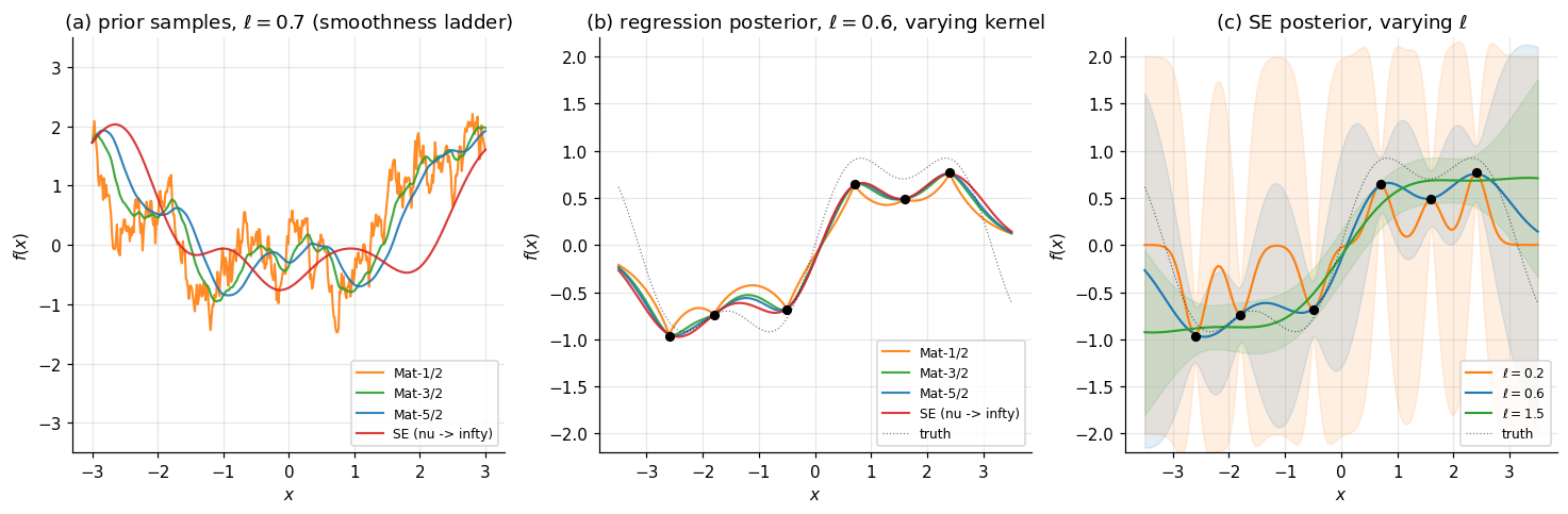
Sweeping ℓ from small (e.g. 0.2) to large (e.g. 1.5) traces the bias–variance axis: too small overfits, too large underfits. The kernel choice axis is orthogonal — Mat-1/2 gives jagged interpolations, Mat-5/2 looks similar to SE in this regime. Toggle bands on to see how each kernel quantifies its own uncertainty in the gaps.

4.3 The working zoo and kernel composition

Beyond the squared-exponential and Matérn families, four other kernels appear in practical work:

Linear kernel. $k_{\mathrm{lin}}(\mathbf{x}, \mathbf{x}') = \sigma_f^2\, \mathbf{x}^\top \mathbf{x}'$. Non-stationary. GP samples are straight lines through the origin with random slope. Rarely used standalone but earns its place as a building block.

Periodic kernel. Defined on one-dimensional inputs (multidimensional generalizations exist but are less common); useful for time series with known seasonality.

White-noise kernel. $k_{\mathrm{wn}}(\mathbf{x}, \mathbf{x}') = \sigma_f^2 \mathbf{1}[\mathbf{x} = \mathbf{x}']$. Adds a $\sigma_f^2$ “spike” to the diagonal. As a kernel component in additive composition it lets us model multiple variance components.

Constant kernel. $k_{\mathrm{const}}(\mathbf{x}, \mathbf{x}') = c$. Encodes a global random-intercept term.

The reason this short list is enough is kernel composition. The space of positive-definite kernels is closed under three operations.

The composition rules are powerful in practice. The classical example is seasonal trend decomposition of atmospheric CO$_2$: $k_{\mathrm{CO}_2}(t, t') \;=\; \underbrace{k_{\mathrm{SE}}}_{\text{long-term trend}} + \underbrace{k_{\mathrm{SE}} \cdot k_{\mathrm{per}}}_{\text{seasonal cycle}} + \underbrace{k_{\mathrm{Mat32}}}_{\text{medium-term irregularity}} + \underbrace{k_{\mathrm{wn}}}_{\text{noise}},$ each component carrying its own lengthscale and amplitude. Rasmussen and Williams 2006 (§5.4.3) develops this exact decomposition in detail.

4.4 Automatic relevance determination

When inputs are multidimensional, the squared-exponential of §2.3 used a single scalar lengthscale for every coordinate. Different features are measured in different units, vary on different scales, and have different relevance. The fix is to give each input coordinate its own lengthscale — the anisotropic or automatic-relevance-determination (ARD) squared-exponential: $k_{\mathrm{SE-ARD}}(\mathbf{x}, \mathbf{x}') \;=\; \sigma_f^2 \exp\!\left(-\frac{1}{2}\sum_{j=1}^d \frac{(x_j - x_j')^2}{\ell_j^2}\right), \qquad \ell_1, \ldots, \ell_d > 0.$ The “automatic relevance determination” name comes from the fact that an irrelevant coordinate $j$ pushes its lengthscale $\ell_j$ to a large value during marginal-likelihood optimization. Inspecting the trained $\ell_j$ values is then a feature-importance diagnostic. The §4 ARD demonstration on synthetic 2D data with one relevant + one irrelevant feature recovers $\ell_1 \approx 1$ for the relevant dimension and $\ell_2 \approx 33{,}000$ for the irrelevant one — the ratio is the diagnostic signal.

ARD generalizes naturally from squared-exponential to the Matérn family (replace $r = \|\mathbf{x} - \mathbf{x}'\|$ with the Mahalanobis distance) and is the canonical multidimensional kernel parametrization in modern GP libraries.

4.5 Choosing a kernel: a small decision tree

1. Smoothness. If the truth is genuinely smooth, use squared-exponential. If smoothness is finite or unknown — the realistic default — use Matérn-5/2. Matérn-3/2 for once-differentiable functions; Matérn-1/2 for Brownian-motion-like processes.
2. Periodicity. If the data have known period $p$, include a periodic kernel component. For quasi-periodic phenomena, multiply periodic by squared-exponential ($k_{\mathrm{per}} \cdot k_{\mathrm{SE}}$).
3. Multidimensional inputs. Use the ARD form by default. Inspect optimized lengthscales as a feature-relevance diagnostic.
4. Multiple variance components. Use kernel addition. A trend + seasonality + irregularity + noise decomposition is the standard structured-time-series template.
5. Linear baseline. When in doubt, include $k_{\mathrm{lin}}$ as an additive component.

§5 takes the kernel as fixed (in functional form) and makes the hyperparameters into things we learn from the marginal likelihood.

5. Learning hyperparameters from the marginal likelihood

§4 introduced the kernel hyperparameters and treated them as quantities we set by hand. The standard fix is to learn the hyperparameters from data by maximizing the marginal likelihood — the probability the training data are assigned by the GP model with those hyperparameters, after the latent function $f$ has been integrated out. §5.1 derives the marginal-likelihood formula. §5.2 reads it as a model-selection criterion (Bayesian Occam’s razor). §5.3 develops the gradient-based optimization. §5.4 returns to the §3 example and recovers $(\sigma_f, \ell, \sigma_n)$ from data.

5.1 The marginal likelihood

Stack the kernel hyperparameters into $\boldsymbol\eta = (\sigma_f, \ell, \sigma_n)$. The marginal likelihood is $p(\mathbf{y} \mid X, \boldsymbol\eta) \;=\; \int p(\mathbf{y} \mid \mathbf{f}, \sigma_n^2)\, p(\mathbf{f} \mid X, \boldsymbol\eta)\, d\mathbf{f}.$ Both factors are Gaussian; the integral is a Gaussian convolution and is closed-form.

The formula has three terms. Data fit: $-\tfrac{1}{2}\, \mathbf{y}^\top \mathbf{A}_\eta^{-1} \mathbf{y}$. Complexity penalty: $-\tfrac{1}{2}\, \log \det \mathbf{A}_\eta$. Constant: $-\tfrac{n}{2}\,\log(2\pi)$. The Cholesky factorization of $\mathbf{A}_\eta = \mathbf{L}\mathbf{L}^\top$ makes the formula computable. The data-fit term factors as $\boldsymbol\beta^\top \boldsymbol\beta = \|\boldsymbol\beta\|^2$ where $\boldsymbol\beta = \mathbf{L}^{-1} \mathbf{y}$; the log-determinant factors as $2 \sum_{i=1}^n \log L_{ii}$. So one $O(n^3)$ Cholesky gives both terms — same cost as a single GP prediction.

5.2 Occam’s razor in the marginal likelihood

The data-fit and complexity-penalty terms trade off in a way that gives GP regression an automatic model-selection mechanism — what MacKay 1992 christened the Bayesian Occam’s razor.

Small $\ell$ (rough functions). $\mathbf{K}$ is close to $\sigma_f^2 \mathbf{I}_n$ — nearly diagonal. $\log \det \mathbf{A}_\eta$ is large in magnitude (very negative complexity penalty), and the model can explain any data, so the data-fit term is also large in magnitude — but the complexity penalty wins. Verdict: the model is too flexible.

Large $\ell$ (very smooth functions). $\mathbf{K}$ has all entries close to $\sigma_f^2$ — rank-1-plus-noise. The complexity penalty is small but the model can essentially only produce constant functions, so the data-fit term is poor. Verdict: too rigid.

Intermediate $\ell$. Both terms are moderate. Verdict: the marginal likelihood prefers this regime, and the optimum recovers the data-correct lengthscale.

This is Occam’s razor for free — the marginal likelihood automatically prefers the simplest model that adequately explains the data, without explicit regularization or held-out validation. The mechanism is purely Bayesian: integrating $f$ out of the joint puts probability mass on the data only to the extent that the model places probability on outputs near $\mathbf{y}$. The marginal-likelihood-as-evidence framing connects directly to Bayesian model comparison (formalstatistics’s formalStatistics: Bayesian Model Comparison and BMA ).

The empirical-Bayes view: maximizing the marginal likelihood with respect to $\boldsymbol\eta$ is type-II maximum likelihood. Full hierarchical-Bayes — putting a prior on $\boldsymbol\eta$ and using HMC — is more principled but computationally expensive (each HMC step is one $O(n^3)$ Cholesky), and in moderately-sized data regimes the marginal-likelihood landscape is concentrated enough that point estimation suffices.

5.3 Gradient-based optimization

Maximizing the marginal likelihood is a numerical optimization problem in $\boldsymbol\eta$. The landscape is non-convex — multiple local maxima exist for non-trivial kernels. Standard recipes: (i) compute analytic gradients (closed-form, much faster than finite differences); (ii) optimize in log-parameter space so positivity constraints on $\sigma_f, \ell, \sigma_n > 0$ are automatic; (iii) run multiple restarts from random initializations.

The analytic gradient is one application of the matrix-derivative identity $\partial_t \mathbf{A}^{-1} = -\mathbf{A}^{-1} (\partial_t \mathbf{A}) \mathbf{A}^{-1}$ and the Jacobi formula $\partial_t \log \det \mathbf{A} = \mathrm{tr}(\mathbf{A}^{-1} \partial_t \mathbf{A})$.

The cost of one gradient evaluation is $O(n^3)$ for the Cholesky plus $O(n^2)$ per hyperparameter for the trace term — same as one function evaluation. Each L-BFGS-B step costs one Cholesky; a typical optimization run is $30$–$100$ Choleskys.

The non-convexity requires care. Two pathologies recur. The flat-likelihood pathology: when $n$ is small, multiple distant $(\sigma_f, \ell)$ combinations can produce comparable marginal likelihoods. The signal-noise confounding pathology: at optima where $\sigma_f$ is small and $\sigma_n$ large, the model attributes all variation to noise; vice versa otherwise. The mitigation is multi-restart optimization: 5–10 random log-space initializations, optimize each to convergence, retain the best.

5.4 Worked example: recovering hyperparameters from data

Returning to the §3 worked example with $n = 30$ training points (the dense set). The data-generating hyperparameters were $\sigma_f = 1.0$, $\ell = 0.6$, $\sigma_n = 0.15$. The §5 question is: with no knowledge of the truth, can the marginal likelihood recover them from the data alone?

Figure 5 has three panels. Panel (a) — marginal-likelihood landscape: a 2D heatmap of $\log p(\mathbf{y} \mid X, \boldsymbol\eta)$ as a function of $(\log \ell, \log \sigma_n)$ at the optimal $\hat \sigma_f$ obtained by profiling. The peak is unambiguous; the contours show the characteristic banana shape with $\ell$ and $\sigma_n$ partially confounded. Panel (b) — recovered posterior with marginal-likelihood-optimized hyperparameters: nearly identical to the §3 hand-set posterior. Panel (c) — optimization curves for five random restarts: all five converge to the same neighborhood despite different starting points.

Run 5-restart L-BFGS optimizerReset to truth

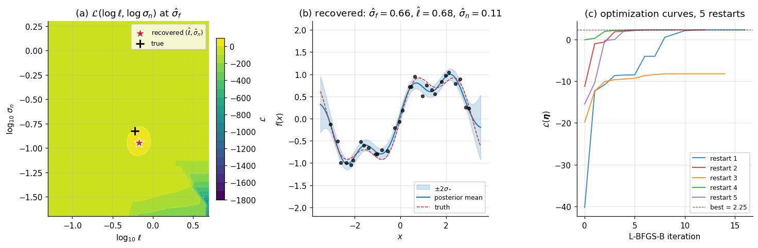
Click anywhere on the landscape to set (ℓ, σ_n) and watch the predictive posterior update in real time. The black "+" marks the truth (ℓ=0.6, σ_n=0.15) and the red "★" tracks your selection. Run the optimizer to overlay all five L-BFGS restart trajectories (start dots → endpoint at the optimum); on this dataset all five converge to the same neighborhood, recovering (σ_f, ℓ, σ_n) ≈ (0.66, 0.68, 0.11).

The recovered hyperparameters are approximately $(\hat \sigma_f, \hat \ell, \hat \sigma_n) \approx (0.66, 0.68, 0.11)$ — within $\sim 25\%$ of the true generating values $(1.0, 0.6, 0.15)$, the right ballpark given the small sample size. With more data ($n = 100$ or $n = 1000$), the optimum sharpens and the recovered values converge to the true ones, as the consistency theory of type-II MLE predicts.

The §5 workflow is the standard recipe for fitting a GP in practice: pick a kernel form (§4), maximize the marginal likelihood for hyperparameters (§5), use the resulting posterior for prediction (§3). For moderate $n$ this is the entire pipeline. When $n$ grows large enough that the $O(n^3)$ Cholesky becomes prohibitive, §6 offers three structural responses.

6. Scaling, neighbors, and limits

§3 ended with the $O(n^3)$ Cholesky bottleneck; §5’s marginal-likelihood optimization is dozens of full Choleskys per fit, multiplying the bottleneck across the optimization loop. For exact GP regression on a single CPU, the practical ceiling is around $n \approx 10{,}000$ — beyond that, both wall-clock time and the $O(n^2)$ memory footprint become prohibitive, and conditioning degrades to the point where ever-larger jitter is needed. The literature has developed several structural responses; this section surveys three. §6.1 covers the Nyström approximation (the spectral baseline, earning its place via the PCA and Low-Rank Approximation prerequisite). §6.2 covers sparse variational GPs (the modern workhorse, earning its place via the Variational Inference prerequisite). §6.3 covers random Fourier features. §6.4–§6.6 lay out neighbors and limits.

6.1 Nyström approximation

The Mercer expansion of §2.4 wrote a kernel as $k(\mathbf{x}, \mathbf{x}') = \sum_{i=1}^\infty \lambda_i \psi_i(\mathbf{x}) \psi_i(\mathbf{x}')$. Truncating at the top $m$ eigenvalues gives a rank-$m$ kernel approximation. The Nyström approximation is the practical version: pick $m \ll n$ inducing inputs $Z = \{\mathbf{z}_1, \ldots, \mathbf{z}_m\}$ (random subsample of $X$, or $k$-means clustering of $X$), define the inducing-block $\mathbf{K}_{mm}$, the cross-block $\mathbf{K}_{nm}$, and the training-block $\mathbf{K}$, and replace $\mathbf{K}$ with the rank-$m$ surrogate $\hat{\mathbf{K}} \;:=\; \mathbf{K}_{nm}\, \mathbf{K}_{mm}^{-1}\, \mathbf{K}_{nm}^\top.$ Equivalently — the connection to PCA and Low-Rank Approximation — $\hat{\mathbf{K}}$ is the projection of $\mathbf{K}$ onto the column space of $\mathbf{K}_{nm}$. The truncation error is controlled by the discarded tail of the kernel-operator spectrum, which decays exponentially for analytic kernels and polynomially for the Matérn family; Drineas-Mahoney 2005 makes this precise.

Predictions through Nyström use $\hat{\mathbf{K}}$ in place of $\mathbf{K}$ with a Woodbury-identity simplification: $\hat{\boldsymbol\mu}_* \;=\; \mathbf{K}_{*m}\,(\mathbf{K}_{mm} + \mathbf{K}_{nm}^\top \mathbf{K}_{nm} / \sigma_n^2)^{-1}\, \mathbf{K}_{nm}^\top \mathbf{y} / \sigma_n^2.$ Cost: $O(nm^2 + m^3)$ per fit, $O(nm)$ memory.

The structural cost is that Nyström is a kernel-matrix approximation, not a probabilistic-model approximation. The implied modified GP has a degenerate kernel matrix and produces over-confident predictive variance. For predictions where uncertainty calibration matters, Nyström’s variance is unreliable. Quiñonero-Candela and Rasmussen 2005 develop this critique in detail; SVGP was developed in response.

6.2 Sparse variational GPs (SVGP)

The modern answer is to wrap the inducing-point construction in the variational machinery of Variational Inference. The construction is due to Titsias 2009; mini-batch SGD by Hensman et al. 2013 scales it to $n \sim 10^6$.

Augment the model with $\mathbf{u} = (f(\mathbf{z}_1), \ldots, f(\mathbf{z}_m))^\top$. The variational family is parametrized over $\mathbf{u}$ alone: $q(\mathbf{u}) = \mathcal{N}(\mathbf{u} \mid \mathbf{m}, \mathbf{S})$, with $q(\mathbf{f}, \mathbf{u}) = p(\mathbf{f} \mid \mathbf{u})\, q(\mathbf{u})$. This factorization embeds the inducing-point assumption directly into the variational family. The ELBO becomes $\mathrm{ELBO}(\mathbf{m}, \mathbf{S}, \boldsymbol\eta, Z) \;=\; \sum_{i=1}^n \mathbb{E}_{q(f_i)}\!\left[\log p(y_i \mid f_i)\right] \;-\; \mathrm{KL}\bigl(q(\mathbf{u})\, \|\, p(\mathbf{u})\bigr),$ with the data-fit term factorizing across training points (one univariate Gaussian expectation per point), allowing mini-batch stochastic gradients. Per-step cost: $O(nm^2 + m^3)$ full-batch, $O(bm^2 + m^3)$ at mini-batch size $b$.

The variational predictive distribution is calibrated: overly-confident predictions are penalized by the KL term, and the construction generalizes immediately to non-Gaussian likelihoods (Bernoulli for classification, Poisson for counts) by replacing the data-fit term with the appropriate expected log-likelihood. SVGP is the substrate of essentially all modern scalable-GP work.

6.3 Random Fourier features

The third response sidesteps inducing points entirely. Random Fourier features (Rahimi-Recht 2007) approximate a stationary kernel by an explicit finite-dimensional inner product. Bochner’s theorem says a stationary kernel is the inverse Fourier transform of a non-negative spectral density $p(\boldsymbol\omega)$: $\tilde k(\boldsymbol\delta) \;=\; \int p(\boldsymbol\omega)\, \cos(\boldsymbol\omega^\top \boldsymbol\delta)\, d\boldsymbol\omega.$ Treating $p(\boldsymbol\omega)$ as a probability density, Monte Carlo estimation gives $k(\mathbf{x}, \mathbf{x}') \;\approx\; \boldsymbol\phi(\mathbf{x})^\top \boldsymbol\phi(\mathbf{x}'), \qquad \boldsymbol\phi(\mathbf{x})_i = \sqrt{\frac{2 \sigma_f^2}{D}} \cos(\boldsymbol\omega_i^\top \mathbf{x} + b_i),$ with $\boldsymbol\omega_i \sim p(\boldsymbol\omega)$ and $b_i \sim \mathrm{Uniform}(0, 2\pi)$. For squared-exponential, $p(\boldsymbol\omega) = \mathcal{N}(\mathbf{0}, \mathbf{I}/\ell^2)$. With features in hand, the problem becomes Bayesian linear regression on $\boldsymbol\phi(\mathbf{x})$ — exactly the §1 parametric model that motivated GPs in the first place, except now the features are randomly sampled to approximate a target kernel rather than chosen by hand.

Cost: $O(nD^2 + D^3)$. Error decays as $D^{-1/2}$. For tasks with moderate kernel hyperparameters, $D \approx 500$–$5000$ recovers near-exact predictive accuracy at training-set sizes that exact GP cannot touch.

The interactive component below sweeps all three approximations against the exact GP baseline at $n = 200$ training points (scaled down from the brief’s $n = 1500$ for browser-side computation). Slide $m$ to watch Nyström and SVGP converge to the exact GP as $m \to n$; toggle methods on/off to compare predictive bands; read fit-time off the per-method labels.

m: 30D (RFF): 150

exact GP · 13.4 msNyström (mean only) · 1.1 msSVGP · 1.8 msRFF · 18.9 ms

Slide m up: Nyström and SVGP converge toward exact GP as m → n. Nyström's variance is omitted because it's structurally overconfident; SVGP and RFF produce calibrated bands. Inducing-point locations are marked along the bottom of the plot. Wall-clock fit-times are reported per method — the takeaway is that for modest m and D, sparse approximations recover near-exact predictive mean accuracy at substantially lower cost than the O(n³) exact GP baseline.

6.4 Within formalML

GPs sit at the junction of several formalML topics.

PCA and Low-Rank Approximation. The Nyström approximation of §6.1 is principal-component analysis applied to the kernel matrix.

Spectral Theorem. The Mercer expansion of §2.4 is the spectral theorem for self-adjoint compact integral operators. Eigenvalue decay (exponential for analytic kernels, polynomial for Matérn) controls Nyström’s convergence rate and RFF’s required feature count.

Variational Inference. The SVGP construction of §6.2 is variational inference applied to GPs. The ELBO of variational-inference is the exact objective Titsias 2009 maximizes.

KL Divergence. The KL term in the SVGP ELBO is reverse KL between two Gaussians, with a closed-form via the multivariate-Normal KL identity.

Forward links to planned T5 topics. GPs are the substrate, in different ways, of:

• Bayesian Neural Networks. The infinite-width limit of a BNN with i.i.d. Gaussian weight priors converges to a Gaussian process (Neal 1996), with a kernel that depends on the activation function and the layer-wise prior variances.
• Neural Tangent Kernel (coming soon). In the infinite-width-and-zero-learning-rate limit of gradient-descent training, the resulting predictive function is exactly a GP with a specific kernel (Jacot et al. 2018) computable in closed form.
• Meta-Learning (coming soon). Neural Processes (Garnelo et al. 2018) are amortized GPs: the variational posterior over $\mathbf{u}$ is the output of an encoder network conditioned on a context set.
• Bayesian Optimization (coming soon, planned T8). The GP is the surrogate model in nearly every modern Bayesian optimization framework.
• Deep Kernel Learning (planned T5). Wilson et al. 2016 proposed a neural network as a feature extractor whose output is fed into a GP kernel.

6.5 Cross-site connections

formalstatistics. The multivariate-Normal density and Gaussian-Gaussian conjugacy that drive §3’s closed-form posterior are the substrate of every formalstatistics Bayesian-conjugate-prior treatment. The marginal likelihood of §5 is exactly the evidence in Bayesian model comparison, and type-II MLE is the empirical-Bayes specialization of the full hierarchical-Bayes treatment. Fully-Bayesian inference over GP hyperparameters via HMC is the natural extension and is precisely what formalStatistics: Bayesian Computation and MCMC covers.

formalcalculus. Bochner’s theorem of §6.3 is harmonic analysis grounded in the Fourier transform machinery of formalcalculus. The Jacobi formula $\partial \log \det \mathbf{A} / \partial t = \mathrm{tr}(\mathbf{A}^{-1} \partial \mathbf{A} / \partial t)$ that drives §5.3’s gradient is a multivariable-calculus identity that appears across statistics and ML.

6.6 Limits and what GPs can’t do

GPs are an extremely capable function-space prior, but they have structural limits worth knowing about up front.

Computational scaling, even with approximations. Exact GPs are $O(n^3)$, capped near $n \approx 10^4$. Sparse approximations push this to $n \sim 10^6$ at the cost of a structural-modeling assumption (the function is well-summarized by $m$ inducing points). None approach the $10^9$-training-point scale of modern deep-learning regression.

Input dimensionality. Standard GP kernels suffer from the curse of dimensionality. The “effective” training-set size for prediction at any test input drops with dimension. Practical GP regression past $d \approx 20$–$50$ requires either a learned feature representation (deep kernel learning), an additive-kernel structural prior, or a different model class.

Non-Gaussian likelihoods. Conjugacy fails for Bernoulli, Poisson, Student-$t$, and most other useful likelihoods. Approximate inference is required — Laplace, expectation propagation, or variational. The §6.2 SVGP machinery is the modern recipe.

Kernel choice as inductive bias. A wrong kernel choice gives wrong predictions, and the marginal likelihood does not protect against gross misspecification. Marginal-likelihood comparison between candidate kernels is the standard mitigation.

Stationarity assumptions. Most practical kernels are stationary. Many real-world functions are not. Non-stationary GP kernels exist but require extra machinery.

No causal structure. The GP’s “prior over functions” has no notion of cause and effect. A GP fit to observational data cannot answer counterfactual questions any better than the observational regression it represents.

GPs are, despite all this, the workhorse function-space prior for moderate-scale ML, the canonical Bayesian regression model, the natural surrogate for Bayesian optimization, and the conceptual scaffold for understanding the infinite-width-network correspondence. The function-space view they introduce — place the prior on the function, not on the parameters — has become the default framing for thinking about uncertainty in regression, even in settings where the underlying machinery is not literally a GP.