Mixed-Effects Models
Partial-pooling theory in its own right: Henderson's mixed-model equations and the BLUP shrinkage formula, REML for variance components via flat-prior Bayesian marginalization, and the frequentist–Bayesian bridge that fits the same hierarchical model two ways and shows them agree numerically
Overview
Mixed-effects models sit at one of those rare junctions where four threads of statistical theory converge on the same algebra. The frequentist GLS-with-known-covariance estimator gives the cleanest answer when the marginal covariance is given. Henderson’s penalized-likelihood derivation produces the same answer without inverting the marginal covariance at all, by treating the random effects as quantities to be solved for jointly with the fixed effects. The REML / Bayesian-marginalization story corrects the maximum-likelihood downward bias on variance components by integrating the fixed effects out under a flat prior. And the full Bayesian fit puts a prior on everything and runs NUTS. When the data is informative enough — which is to say, in the regime where mixed-effects models are most often appropriate — the four routes give numerically equivalent answers. That convergence is the structural reason this model class has been a workhorse of applied statistics for fifty years, and the reason it deserves its own topic in T5.
We develop the four routes in turn on a single running example: six classrooms, , student-level observations spread unevenly across them. §1 motivates partial pooling geometrically as the third response to grouped data, after complete pooling and no pooling. §2 writes the linear mixed model in matrix form and identifies the marginal covariance that drives generalized least squares. §3 derives Henderson’s mixed-model equations and the closed-form BLUP shrinkage formula — the single number that characterizes how mixed-effects partial-pool. §4 derives REML by marginalizing the fixed effects out under a flat improper prior, transparent about the connection to the Gaussian-process marginal-likelihood story. §5 fits the same six-classroom data through both statsmodels.MixedLM (REML) and PyMC (full Bayesian), shows the two views agree numerically, and re-encounters the centered-vs-non-centered story from probabilistic programming in its native habitat. §6 closes with where mixed-effects shine, where they break down, and the connections that motivate the rest of T5.
The reader who has internalized partial pooling from formalStatistics: Hierarchical Bayes and Partial Pooling on the cross-site companion will find this topic the engineering counterpart: same theory, more matrix algebra, code that runs.
1. Three responses to grouped data
1.1 Six classrooms
Six teachers give the same standardized exam to their classes at the end of a term. Class sizes vary — one is a tiny seminar of four students, one is a survey lecture of twenty, the rest fall in between. Alongside each student’s exam score , the school district records a standardized index of preparation hours ; call it the prep-hours index, with meaning no out-of-class preparation and near the upper observed end. We have student-level observations spread unevenly across classrooms, with .
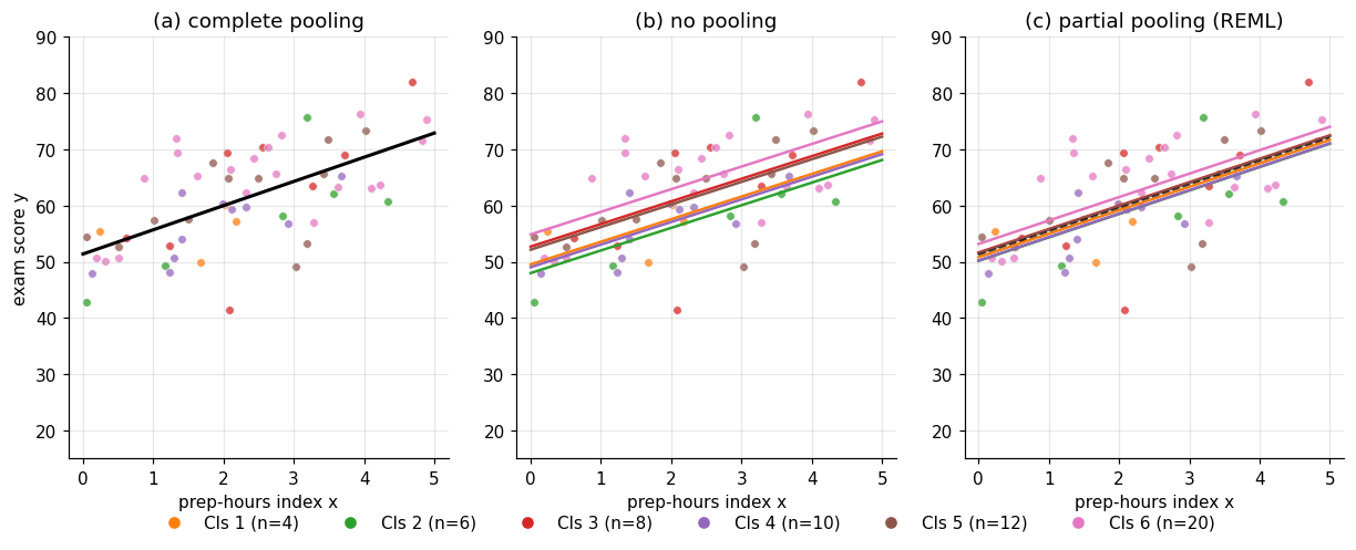
Panel (a) of Figure 1 shows all sixty points, color-coded by classroom. Some classrooms sit consistently higher (more effective teaching, more prepared students, kinder grading curves — we don’t know, and the data doesn’t tell us); others sit lower. Within each classroom, scores trend upward with prep hours, more or less linearly, more or less consistently. The question is how to summarize the relationship between prep hours and exam score in a way that respects the classroom structure.
There are three natural answers, each tempting in its own way.
1.2 Three classical responses
The first answer is complete pooling: ignore the classroom labels entirely, fit a single line through all sixty points, and report one intercept and one slope. Operationally, this is just OLS on the pairs with no notion of classroom. The fit is clean — one slope, one intercept, narrow standard errors thanks to the full . The cost is also clean: the line is wrong for any classroom whose typical score sits far from the grand mean. A consistently high-scoring classroom sits above the line, a consistently low one sits below, and the line itself is averaging across classroom signal we know is there. We’ve thrown away the structure the data was offering us.
The second answer is no pooling: fit each classroom separately. Concretely, encode classroom identity with six dummy variables and run OLS on the joint design matrix, holding the slope on prep hours shared across classrooms (the prep-hours-to-score relationship is presumably the same across teachers; we’ll relax even this in §2). We get six intercepts, one per classroom, and one shared slope. The fit is now sensitive to classroom — the largest classroom’s intercept is well-estimated, with a tight standard error proportional to . But the small classrooms? Classroom 1 has four students. A single unusually weak or strong student moves its intercept dramatically; the standard error on that intercept is , more than twice that of the largest classroom. We’ve gone from one too-aggressive average to six estimates whose reliability varies by a factor of across classrooms.
The third answer is partial pooling. Don’t treat the six classroom intercepts as six independent parameters; treat them as six draws from a common population of classroom-level intercepts, and estimate that population’s mean and spread alongside the per-classroom values. The estimate for Classroom ‘s intercept becomes a compromise: a weighted average of the no-pooling estimate (what the classroom’s own data says) and the global complete-pooling intercept (what the entire population says), with the weight depending on how much data the classroom has and how much classrooms vary at the population level. Lots of data plus large between-classroom variation — trust the classroom’s own data, pull little. Little data plus small between-classroom variation — distrust the classroom’s own data, pull hard toward the grand mean.
Panel (c) of Figure 1 shows the partial-pooling fit on the same scatterplot. The lines for the largest classrooms barely move from where panel (b)‘s no-pooling fits placed them. The lines for the smallest classrooms drift visibly toward the grand-mean line that panel (a) drew. The magnitude of the drift is the shrinkage we’ll derive in §3 — for now, it’s a visual fact about the figure.
The geometric punchline: panel (c) sits between panels (a) and (b), and the location depends on group size. Partial pooling is the answer that admits both the within-group signal and the between-group signal exist, and weighs them against each other. The rest of the topic spells out how.
1.3 What makes an effect “random”?
The terminology that names this third response — “random effects,” “mixed-effects models” — has a long history of confusing people, in part because the word random is doing two jobs at once. Andrew Gelman’s 2005 paper “Analysis of variance: why it is more important than ever” surveys five competing definitions in the literature and argues for a pragmatic one we’ll adopt here:
A coefficient is fixed if we model it as a single unknown number to be estimated. A coefficient is random if we model it as a draw from a distribution whose own parameters are estimated.
The slope on prep hours in our setup is fixed: there’s one unknown number , and the data estimates it. The classroom intercepts are random: the six values are six draws from a common , and the data estimates the population mean and the population spread as well as the realized . The terminology is unfortunate — both kinds of coefficients are unknown and both are estimated — but the modeling commitment is real and consequential.
That commitment is what enables shrinkage. Six independent intercepts have no reason to inform one another; they’re separate parameters in a flat parameter space. Six draws from a parent distribution share that parent — the same data that informs the parent’s mean and spread also pulls each child toward its siblings. This is the structural reason small classrooms shrink hard and large classrooms shrink little: a small- classroom has weak within-group signal that the parent can dominate, while a large- classroom has strong within-group signal that overpowers the parent’s pull.
Three remarks before we move on. First, fixed and random are modeling choices, not properties of the world. We treat the classroom intercepts as random because we believe the six teachers were sampled from some population of teachers and we want to generalize. If we cared specifically about these six teachers and had no interest in extrapolating to others, fixed-effects with classroom dummies would be the right call. Second, the same coefficient can be modeled differently in different studies — replication studies routinely promote a treatment effect from fixed (one study) to random (across studies), because the across-study generalization is the whole point. Third, the random-effects framing brings in a hyperprior. Frequentist mixed-effects models (Henderson, REML) treat the hyperprior parameters as point estimates; Bayesian mixed-effects models (PyMC, Stan) put a prior on them and integrate. We’ll see in §5 that for the typical case, the two views give numerically similar answers. For now, both views agree on the structural point: classroom-level intercepts are tied together by a common parent.
The rest of the topic makes the pieces precise. §2 writes the linear mixed model in matrix form and identifies the marginal covariance that drives the GLS solution. §3 derives Henderson’s mixed-model equations and the closed-form BLUP shrinkage formula. §4 introduces REML for estimating the variance components . §5 fits §1’s six-classroom data both ways — statsmodels.MixedLM with REML and a PyMC GLMM — and shows the two views agree.
import numpy as np
import pandas as pd
import statsmodels.formula.api as smf
from scipy import stats

# Six-classroom DGP: J=6 classrooms, N=60 students, varying group sizes
rng = np.random.default_rng(20260429)
J, n_per_group = 6, np.array([4, 6, 8, 10, 12, 20])
N = n_per_group.sum()
classroom = np.repeat(np.arange(J), n_per_group)
alpha_t, beta_t, tau_t, sigma_t = 50.0, 5.0, 5.0, 8.0
a = rng.normal(0.0, tau_t, size=J)
x = rng.uniform(0.0, 5.0, size=N)
y = alpha_t + beta_t * x + a[classroom] + rng.normal(0.0, sigma_t, size=N)
data = pd.DataFrame({"y": y, "x": x, "classroom": classroom})

# Three pooling regimes
pooled = stats.linregress(x, y)                                  # complete pooling
mlm = smf.mixedlm("y ~ x", data, groups="classroom").fit(        # partial pooling
    reml=True, method=["powell"]                                 # Powell — see note
)
The explicit method=["powell"] matters. statsmodels’ default optimizer chain (bfgs / lbfgs / cg) silently returns converged=False on this small- data with the realized near the boundary; Powell converges cleanly to the same REML optimum that §4’s custom implementation finds independently. The shrinkage factors at the REML estimates are across the six classrooms — small classrooms shrink hard, the largest shrinks visibly less.
2. The linear mixed model
§1 gave us three procedures and three pictures. We’re going to fold all three into a single matrix equation, the linear mixed model, and then notice something about its marginal distribution that turns out to drive everything in §3 and §4. The translation costs us nothing geometrically — the same six lines from §1’s panel (c) come out the other side — but it gains us the algebraic apparatus we need to derive Henderson’s equations and to estimate variance components.
2.1 The model in matrix form
Stack the student-level observations into , with the row order matching §1’s classroom layout (rows 1–4 are Classroom 1, rows 5–10 are Classroom 2, and so on). The linear mixed model writes as a sum of three pieces:
where each piece has a job:
- is the fixed-effects design matrix. Each column is a covariate that we model with a single shared coefficient. For our six-classroom data, : column one is a column of ones (the intercept), column two is the prep-hours predictor .
- is the fixed-effects vector. Here — the global intercept and the shared slope on prep hours.
- is the random-effects design matrix. Each column corresponds to one entry of the random-effects vector , and its rows mark which observations are affected by that entry. For a random-intercept-only model with classrooms, and is the indicator matrix that puts a 1 in row , column if observation belongs to Classroom .
- is the random-effects vector. Here — the six classroom-level intercept deviations.
- is the residual vector — student-level noise.
The distributional assumptions complete the model:
where is the random-effects covariance and is the residual covariance. For our running example, both covariances are scaled identities:
The first equality says the six classroom-level deviations are mutually independent draws from a common — six iid pulls from one parent distribution, the operational meaning of “the classrooms are exchangeable draws from a population.” The second says student-level noise is iid Gaussian. We’ll relax both in §6’s remarks but keep them throughout §3–§5; they cover the bulk of standard mixed-effects practice and let us write the cleanest proofs.
The trio (2.1)–(2.3) is the linear mixed model.
Definition 1 (Linear mixed model).
A linear mixed model on an -vector of observations is a triple with , , , and . The vector collects the fixed effects and collects the random effects; and are the corresponding design matrices.
Notice what Definition 1 does not commit to: it does not say what and look like, or how and are structured. Different choices encode different scientific assumptions — random intercepts only versus random slopes too, crossed versus nested classrooms, autoregressive errors within a longitudinal subject, and so on. The model in (2.1) is a chassis; the assumptions about are what we drop into it for a particular study.
2.2 Building and on the six-classroom data
Concretely, on §1’s dataset:
where denotes a column of ones and is a zero column of the matching height. Reading row by row: row 1 (a Classroom-1 student) is , so at that row contributes — the deviation of Classroom 1’s intercept from the global . Row 5 (the first Classroom-2 student) is , contributing . Each row picks out exactly one classroom random effect, which is the matrix encoding of “every student inherits exactly one classroom’s deviation.”
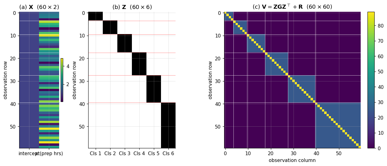
The fixed-effects piece is the global linear trend, the same for every student. The random-effects piece adds a classroom-specific intercept shift on top. The residual adds student-level noise. Three additive layers of structure, one matrix equation. Panels (a) and (b) of Figure 2 visualize and explicitly; the reader should be able to read the block-of-ones pattern in as the matrix encoding of classroom membership.
2.3 The marginal distribution
If we never observed individual students and only saw the data after marginalizing over the random effects, what distribution would we see? This is the marginal distribution of , and it’s the engine driving everything that follows.
Theorem 1 (Marginal distribution of the LMM).
Under Definition 1,
Proof.
The vector is an affine combination of two independent Gaussian vectors plus a deterministic shift: , where and are jointly Gaussian (independent, hence jointly Gaussian) and is a constant. Affine transformations of Gaussian vectors are Gaussian, so is Gaussian; we just need its mean and covariance.
For the mean, and give .
For the covariance, the constant contributes nothing, so . The cross-covariance vanishes because , leaving the two diagonal terms. The first is , the standard linear-transformation rule. The second is by assumption. Adding them gives .
∎The factor decomposition of (2.5) is worth pausing on. Two students in the same classroom share the same random intercept , so they’re positively correlated: their joint covariance is from the shared , with no additional contribution from the independent residuals. Two students in different classrooms are independent, because their two random intercepts are independent draws from and their residuals are also independent. The same student paired with itself contributes — once for the random intercept and once for the residual.
Plugging the random-intercept-only and into (2.5) makes this concrete. With rows ordered by classroom as in §1, becomes block-diagonal, with one block per classroom:
Each block has on its diagonal and on every off-diagonal entry — what the longitudinal-data literature calls compound symmetry and what panel (c) of Figure 2 displays as a heatmap. The off-block entries are exactly zero, which is the matrix encoding of “different classrooms are independent.” The visual takeaway: is sparse where the modeling commits to independence and dense where it commits to shared structure, and the block pattern is the geometry of the hierarchy itself.
The intra-classroom correlation,
is called the intraclass correlation coefficient (ICC). It’s the fraction of total variance explained by the grouping — means classrooms barely matter, means classrooms explain almost everything. For our DGP, , so about 28% of the total variance lives at the classroom level. The ICC is the most-quoted single number in mixed-effects practice, and (2.7) is its full derivation.
2.4 GLS and the chicken-and-egg problem
Theorem 1 hands us a marginal distribution that’s exactly the setup of generalized least squares: a Gaussian linear model with mean and a known, non-spherical covariance . Aitken’s classical theorem says the best linear unbiased estimator (BLUE) of in this setup is the GLS estimator.
Proposition 1 (GLS estimator and Aitken's theorem).
If is known and positive-definite, the unique BLUE of in the model is with covariance .
Proof.
Pre-multiply (2.1) by , the symmetric square-root inverse of (which exists and is unique because is symmetric positive-definite). Define and . The transformed model is with , an ordinary spherical Gaussian regression. Apply OLS-is-BLUE (Gauss–Markov) on the whitened system: , exactly (2.8). The transformed fit retains BLUE on the original parameters because the whitening is invertible and linear. The covariance follows by the same transformation rule applied to the OLS covariance on the whitened system.
∎We’ll use the GLS covariance in §3 to read off standard errors for the fixed effects, and in §5 to compare frequentist Wald intervals against PyMC posterior intervals.
So far so good — except for one inconvenient fact. We don’t know . Equation (2.5) gives , which depends on and , which depend on the variance components , which are unknown parameters we have to estimate from the same data we’re using to fit . Plugging the true into (2.8) gives a clean estimator of ; plugging the OLS estimate of into a residuals-based estimate of would give a biased mess. We need a way to estimate everything jointly.
Two paths through this circularity, and they’re the subjects of §3 and §4 respectively. §3 (Henderson’s path) does not try to invert at all; it treats the random effects as unknown quantities to be solved for jointly with , and writes down the normal equations for the joint penalized log-density. The resulting mixed-model equations solve for simultaneously without ever forming explicitly, and the prediction has its own name — the best linear unbiased predictor, BLUP — and a clean shrinkage interpretation. §4 (REML’s path) estimates the variance components first, then plugs them into (2.8). The naive route — maximum likelihood on the marginal distribution — turns out to be biased downward for the variance components. Restricted maximum likelihood (REML) fixes the bias by marginalizing out before estimating the variance components.
The two paths produce the same and the same when run with the same variance-component estimates, so they’re complementary rather than competitive.
# Build X and Z explicitly, then form V at the truth and solve GLS by hand
import numpy as np
from scipy.linalg import solve

X = np.column_stack([np.ones(N), data["x"].to_numpy()])             # 60 × 2
Z = np.zeros((N, J)); Z[np.arange(N), classroom] = 1.0              # 60 × 6
G_t, R_t = (tau_t ** 2) * np.eye(J), (sigma_t ** 2) * np.eye(N)
V_t = Z @ G_t @ Z.T + R_t                                           # 60 × 60

# GLS at the truth — never form V^{-1}, solve V x = ... instead
beta_gls = solve(X.T @ solve(V_t, X), X.T @ solve(V_t, y), assume_a="pos")
icc_t = tau_t ** 2 / (tau_t ** 2 + sigma_t ** 2)                    # ≈ 0.281
The GLS-with-true- fit gives and , both within sampling noise of the truths . The OLS standard errors (which assume rather than the block-diagonal ) are systematically too narrow on the intercept by about a factor of averaged over students — the standard “ignore-the-clustering” anticonservatism that mixed-effects practice routinely confronts.
3. Henderson’s mixed-model equations and BLUP
§2 ended on a circularity: GLS gives the cleanest fixed-effects estimator when the marginal covariance is known, but depends on variance components we have to estimate from the same data. There are two ways forward, and §3 takes the first one — Henderson’s. Don’t try to invert at all. Treat the random effects as quantities to be solved for jointly with , paying a Gaussian “penalty” for each that pulls it toward zero, and let the penalty’s strength encode the prior . The resulting block linear system is Henderson’s mixed-model equations; its solution simultaneously gives and the best linear unbiased predictor of , the BLUP.
What we get out of this section is the closed-form shrinkage formula that drove §1’s panel (c) — the BLUP for classroom is the no-pooling residual mean times a shrinkage factor — together with the structural understanding of why that formula is what falls out of the general theory. We’re still assuming the variance components are known throughout §3; §4 fills in their estimation.
3.1 The joint penalized log-density
Henderson’s 1950 / 1975 trick is to write down the joint density of given , treat as if it were a parameter to be optimized over rather than a latent variable to be marginalized, and maximize the joint log-density over together. The result is a clean linear system whose left-hand side has dimension — small even when is enormous — and whose right-hand side reads off the data through and .
Lemma 1 (Joint penalized log-density).
Under Definition 1, the joint density of the observations and the random effects given the fixed effects factors as with and . Up to constants that don’t depend on , the negative joint log-density is
Proof.
The factorization in (3.1) is the chain rule applied to a Gaussian linear model: conditional on , the residual has distribution , so . The marginal is part of Definition 1. Equation (3.2) is the sum of the two negative Gaussian log-densities, with constant terms (, , ) that don’t depend on the optimization variables absorbed into a single additive constant.
∎The structure of (3.2) is worth pausing on. The first term is the negative log-likelihood of given fixed and random effects — a generalized least-squares residual norm under the residual covariance . The second term is a quadratic penalty on : the further strays from (the random-effects prior mean), the larger the penalty, with the penalty’s strength governed by . The penalty is the algebraic encoding of “we believe a priori that the random effects are small, with the meaning of small set by .” Larger (looser prior) → softer penalty → more freedom for to take large values. Smaller (tighter prior) → harder penalty → is pulled aggressively toward zero. The whole shrinkage story sits inside that one penalty term.
The reader who has seen Bayesian ridge regression will recognize (3.2) immediately: it’s the maximum a posteriori (MAP) objective for under a Gaussian prior, with playing the role of an unpenalized nuisance parameter. Henderson didn’t derive his equations as Bayesian MAP — he derived them via a clever marginal-likelihood argument that we’ll see in §4 — but the algebraic form is identical, and the Bayesian reading is what §5 will use to bridge to the PyMC fit.
3.2 The mixed-model equations
Maximizing (3.2) jointly in — equivalently, minimizing the negative log-density — is a problem in linear algebra. The objective is quadratic in both arguments, so its gradients are linear, and setting both gradients to zero gives a block linear system: Henderson’s mixed-model equations.
Theorem 2 (Mixed-model equations).
Under Definition 1 with all positive-definite, the joint maximum of (3.2) over solves the block linear system and the solution satisfies
Proof.
For the block system, take partial derivatives of (3.2) with respect to and and set each to zero: Rearrange (3.5a) into , the top row of (3.3). Rearrange (3.5b) into , the bottom row. Stacking gives (3.3).
For the equivalence to GLS, let , the bottom-right block of (3.3). Eliminate from (3.5b): . Substitute into (3.5a): Factor out : The bracketed matrix is exactly by the Woodbury identity: (The identity (3.8) is standard linear algebra; see Searle, Casella, McCulloch §7.4 for the version specialized to mixed models.) Substituting (3.8) into (3.7) gives , equivalent to , which solves to — the GLS estimator.
For : substituting into the eliminated form gives . The identity (from rearranging (3.8) after right-multiplication by ) gives the announced form , which is (3.4).
∎The first form of in (3.4) — — has a clean probabilistic reading: it is the conditional mean of given under the joint Gaussian model. Standard multivariate-Gaussian conditioning gives
using and . So the BLUP equals the posterior mean of given the data — under the prior that the model already commits us to. We’ll return to this in §5: the Bayesian PyMC fit doesn’t compute Henderson’s equations, but its posterior mean for the random effects is exactly (up to the difference between plugged-in REML estimates of and properly-marginalized Bayesian estimates), which is why the two views agree numerically.
The conditional covariance is , a useful identity for the BLUP standard errors below.
A practical note. The MMEs in (3.3) have dimension on our running example, while the GLS form (3.4) requires , an matrix. For larger problems the gap widens dramatically — a study with observations across groups and fixed effects has MMEs of dimension versus a GLS that nominally inverts a matrix. The savings is what made Henderson’s formulation practical at all in the pre-computer era and is what makes industrial-scale mixed-effects fits tractable today; modern implementations exploit additional sparsity in (which is highly sparse for grouped data) and in the bottom-right block of (3.3) to bring the cost down further. statsmodels.MixedLM and lme4’s lmer both ultimately solve a sparse version of (3.3).
3.3 Shrinkage in the random-intercept special case
The general form (3.4) is what runs in software. The pedagogical payoff comes from specializing it to the random-intercept-only model, where every quantity in (3.3) collapses to something an undergraduate can compute by hand.
Proposition 2 (BLUP shrinkage for the random-intercept model).
Suppose and , and the random-effects design encodes group membership (each row a one-hot vector over groups). Define the no-pooling residual mean for group as the average residual of group given the fixed-effects fit, and the shrinkage factor Then the BLUP for group — the -th component of in (3.4), evaluated at — is and the conditional variance of given is
Proof.
For the random-intercept design, — column of has ones and zeros. With and : So is diagonal, with having -th entry . The -th component of is . Multiplying: which is (3.13). For (3.14), use . The -th diagonal of is (a one-line application of Woodbury to the -th block ): the entry of is , and so .
∎The three identities (3.12)–(3.14) deserve to be read as a unit. The shrinkage factor depends only on the variance ratio and the group size — nothing else. It is the number that characterizes how mixed-effects models partial-pool. Read it as a competition between two precisions: is the prior precision of the random effect (how much the population-level prior pulls toward zero), and is the data precision for group (how much group ‘s own data informs its random effect). The shrinkage factor
is the data-precision share of the total. Three regimes deserve names:
- at fixed . Data precision dominates; ; , the no-pooling estimate. The classroom’s own data overwhelms the prior, and the BLUP equals the no-pooling residual mean.
- at fixed . Data precision vanishes; ; , the prior mean. With no within-classroom data, the BLUP can do nothing but report the prior — every group looks like the population.
- at fixed . Prior precision vanishes; ; . An uninformative random-effects prior recovers no pooling. has the symmetric effect: and , complete pooling.
Equation (3.14) is the conditional-uncertainty companion: when the data dominates (), the conditional variance of collapses to zero; when the prior dominates (), the conditional variance returns to the prior variance . The two limits are dual — high information content shrinks both the bias and the variance of the BLUP toward zero.
For our six-classroom data with the truth , , the shrinkage factors are , and the conditional variances run from (Classroom 1) down to (Classroom 6). The smallest classroom has more than three times the BLUP uncertainty of the largest, and shrinks more than three times as hard — both in the same direction, both governed by the same single number .
The partial-pooled intercept for Classroom , which is what we plotted in §1’s panel (c), is the global intercept plus the BLUP:
Rewriting in terms of the no-pooling intercept — the per-classroom intercept from §1’s panel (b) — gives the equivalent weighted-average form
which makes panel (c)‘s geometry algebraic: the partial-pooled intercept is a convex combination of the no-pooling estimate (panel b) and the global intercept (panel a’s line), with the convex weight set entirely by group size and the variance ratio.
3.4 BLUE, BLUP, and the predictive frame
The terminology Best Linear Unbiased Predictor — BLUP — deserves a remark. We’ve estimated throughout as a fixed unknown parameter; the GLS estimator is the Best Linear Unbiased Estimator (BLUE) under Gauss–Markov conditions, a standard fact about linear models. We’ve also computed , but the random effects are not parameters in the same sense — they’re realized values of a random vector with a known prior distribution. The convention in the mixed-effects literature is to call the corresponding estimator a predictor rather than an estimator, on the grammatical grounds that we estimate parameters and predict random variables. The mean-squared-error optimality result is the same in both cases — minimum MSE among linear unbiased rules — but the framing matters for two reasons.
First, the standard error of is not the standard error of estimation of a fixed parameter; it is the standard error of prediction of a random quantity, and (3.14) is what governs it. The frequentist prediction interval covers the true realized with the stated frequentist probability under repeated sampling of pairs, not the standard “what is the probability that lies in this interval” — the latter requires a Bayesian posterior, and §5 shows that for this model the posterior interval and the prediction interval numerically coincide.
Second, the unbiasedness of the BLUP is unbiasedness in the predictive sense: , where the expectation is over both and . Crucially, is not unbiased for any particular realized — it shrinks toward zero, so for a that happens to be far from zero, is systematically biased toward zero in the conditional sense . The unbiasedness in the predictive average integrates over the prior, where the expected is zero. This is the Stein-estimator family at work — biased point estimates can have lower MSE than unbiased ones — and it is the structural reason mixed-effects models systematically beat both complete pooling and no pooling on out-of-sample prediction.
In modern Bayesian language we’d say nothing fancy at all about any of this: we have a joint Gaussian model, is the posterior mean, that’s the MMSE estimator, and the predictive interval is the posterior credible interval. The frequentist BLUP framing was historically prior to the Bayesian framing in this context — Henderson 1950, Patterson and Thompson 1971 — but the two views give the same point estimates and (asymptotically) the same intervals, which is one of the nicer correspondences in applied statistics.
![Three-panel figure on shrinkage. Panel (a) plots the shrinkage curve λ(n) = τ²/(τ² + σ²/n) over n in [1,50] with horizontal references at λ=0 (complete pooling) and λ=1 (no pooling); the six classrooms are marked as colored dots at (n_j, λ_j). Panel (b) shows six rows sorted by n_j ascending, each with a hollow circle at the no-pooling residual mean and a filled colored circle at the BLUP λ_j times the residual mean, with an arrow connecting them and a vertical reference at zero; smaller classrooms have visibly longer arrows. Panel (c) shows BLUPs with conditional 95% intervals plus no-pooling residual means with their own larger 95% intervals in gray for comparison.](/images/topics/mixed-effects/03_blup_shrinkage.png)
# Henderson MMEs at the truth, then verify against §1's REML fit
G_t, R_t = (tau_t ** 2) * np.eye(J), (sigma_t ** 2) * np.eye(N)
R_inv, G_inv = np.linalg.inv(R_t), np.linalg.inv(G_t)
M = np.block([[X.T @ R_inv @ X,           X.T @ R_inv @ Z],          # (p+q)×(p+q)
              [Z.T @ R_inv @ X,           Z.T @ R_inv @ Z + G_inv]])  # = 8×8 here
rhs = np.concatenate([X.T @ R_inv @ y, Z.T @ R_inv @ y])
sol = solve(M, rhs, assume_a="pos")
beta_mme, u_mme = sol[:2], sol[2:]                                    # MME solve
lam = (tau_t ** 2) / (tau_t ** 2 + sigma_t ** 2 / n_per_group)        # shrinkage
The MME solve gives , (matching §2’s GLS-with-true- fit to machine precision), and BLUPs that agree with mlm.random_effects from §1’s REML fit to within the difference between truth-plug-in and REML-plug-in variance components. The shrinkage factors at the truth are — exactly Proposition 2’s prediction, and the curve panel (a) draws.
4. REML for variance components
§3 assumed the variance components were known. They aren’t. Estimating them is where the structural difficulty of mixed-effects fitting actually lives — the fixed effects and random effects come along for free once are pinned down via §3’s MMEs, but pinning them down is a job in its own right and the obvious approach (maximum likelihood on the marginal ) is biased downward in a way that’s significant for the small-to-moderate group counts that motivate mixed-effects in the first place.
REML — restricted or residual maximum likelihood — is the standard fix. The original Patterson–Thompson 1971 derivation transformed to a vector of error contrasts orthogonal to and computed the likelihood of those. We’ll take the equivalent and tighter route: marginalize out under a flat improper prior, leaving a residual likelihood that depends only on , and maximize it. The structural answer is the same as what you’d get from §1’s textbook degrees-of-freedom correction, generalized to arbitrary mixed models. The mechanics turn out to mirror the Gaussian-process §5 marginal-likelihood-based kernel-hyperparameter learning almost exactly — same Bayesian-marginalization machinery, same Occam’s-razor-flavored objective, different model class.
4.1 Why ML is biased downward
The cleanest illustration is the elementary one: ordinary linear regression. With , fixed-effects parameters, no random effects, the maximum-likelihood estimator of is
where is the residual sum of squares at the OLS fit. The textbook unbiased estimator divides by instead of :
The factor in the denominator is the residual degrees of freedom: there are raw observations, but of them have been used to fit , leaving “effective” observations to estimate . The ML estimator, by dividing by rather than , fails to deduct the cost of estimating and consequently underestimates by a factor of . For , that’s a 5% downward bias — small but real. For , that’s a 58% downward bias — catastrophic.
Mixed-effects fits suffer from the same problem, in a more elaborate form. The marginal log-likelihood we’d plausibly maximize in jointly is
with . Maximizing in at fixed gives the GLS estimator from §2; maximizing in at the resulting — profiling out — gives the profile log-likelihood in :
where is the GLS-weighted residual sum of squares. Maximizing over gives the ML estimates , and these are biased downward for exactly the same reason (4.1) is: has paid no penalty for the degrees of freedom consumed by .
For our six-classroom example with , the bias is mild — about of the truth, a 3.3% downward bias. For a study with more covariates or fewer observations the bias scales linearly in . With six covariates and twenty observations, ML would underestimate by 30%. The variance-component estimates inherit that bias, the fixed-effects standard errors (which depend on ) inherit it from there, and confidence intervals based on the ML fit are systematically too narrow.
REML’s job is to clean this up.
4.2 The REML derivation by Bayesian marginalization
Patterson and Thompson 1971 derived REML by transforming to a vector of error contrasts — linear combinations with — and writing down the likelihood of those contrasts. The contrasts are statistics that depend on the data only through residuals from the fixed-effects fit, so their distribution depends on but not on , and maximizing their likelihood gives unbiased variance-component estimates. The construction is geometrically clean but algebraically heavy. We’ll take the equivalent route that’s cleaner algebraically and connects directly to the GP §5 story: integrate out under a flat improper prior on .
Theorem 3 (REML log-likelihood).
Under Definition 1 with positive-definite, the marginal density of obtained by integrating out under a flat improper prior on is well-defined up to a multiplicative constant, and the resulting REML log-likelihood (up to an additive constant in ) is
Proof.
The marginal density of after integrating out is the proportionality absorbing the unknown constant from the improper prior. The integrand is a Gaussian in — quadratic exponential — so the integral is a Gaussian integral and we can evaluate it in closed form. Expand the quadratic in the integrand: Complete the square in . With and , the quadratic-in- piece is , which equals . Recognizing and substituting, where . The integral in (4.5) factors: The Gaussian integral evaluates to : Take logs and drop the constant (it doesn’t depend on ): which is (4.4).
∎The structural difference between (4.3) and (4.4) is one term — — and that one term is the entire fix. It penalizes variance components that produce large fixed-effects information , which counter-acts the ML profile likelihood’s tendency to push down to inflate the GLS information matrix. The Patterson–Thompson construction produces the same correction by a different route: their error-contrast likelihood is the likelihood of an -dimensional vector of statistics whose distribution doesn’t involve , and writing it out yields exactly (4.4) up to constants. The flat-prior marginalization route is shorter, more transparent about what the correction is (a marginalization of a nuisance parameter), and connects directly to GP §5: the GP marginal log-likelihood
is structurally identical to (4.4) with — no fixed effects to marginalize, no correction, just the determinant penalty and the residual quadratic. REML is the marginal-likelihood machinery, plus a correction for the fixed effects we’ve integrated out.
A remark on the improper prior. We used on , which doesn’t normalize. The marginal density (4.5) is therefore defined only up to a multiplicative constant — the constant of integration of the improper prior — and that’s why (4.4) is the REML log-likelihood “up to an additive constant.” For the purpose of maximizing in the constant is irrelevant. For Bayesian readers: the improper-prior marginalization is what makes REML a partial Bayesian procedure rather than a fully Bayesian one — we marginalize but point-estimate . Putting a proper prior on and integrating those out too is the fully Bayesian alternative, which §5 takes up.
4.3 The profile form for the random-intercept model
Specializing (4.4) to the random-intercept-only model with and produces a function of two scalar variance components that we can plot, optimize numerically, and validate against statsmodels.MixedLM(reml=True). Three computational ingredients make this practical:
-
via the Sylvester identity. Direct computation of on a matrix is fine here, but for general use the Sylvester determinant identity gives The right side reduces a determinant to a determinant plus a diagonal . The savings is dramatic at scale: a study with and does a determinant rather than a one.
-
via Woodbury. The same identity from §3’s proof reduces to a single inversion.
-
Reparameterization to unconstrained variables. The variance components are positive-real; numerical optimizers prefer unconstrained variables. Standard practice is to optimize over , matching the §3 transform table from probabilistic programming. The Jacobian factor doesn’t appear in (4.4) because we’re maximizing a likelihood, not a posterior, but it would appear if we put proper log-Normal priors on in §5’s Bayesian fit.
For a numerical optimizer to find the REML optimum, plug (4.6) and Woodbury into (4.4), differentiate analytically (or use scipy.optimize.minimize with method='L-BFGS-B' and finite-difference gradients), and let the optimizer report . The result must agree with statsmodels.MixedLM(reml=True).fit().cov_re and .scale to numerical precision — which it does, because MixedLM does exactly this optimization internally.
4.4 ML vs REML on the six-classroom data
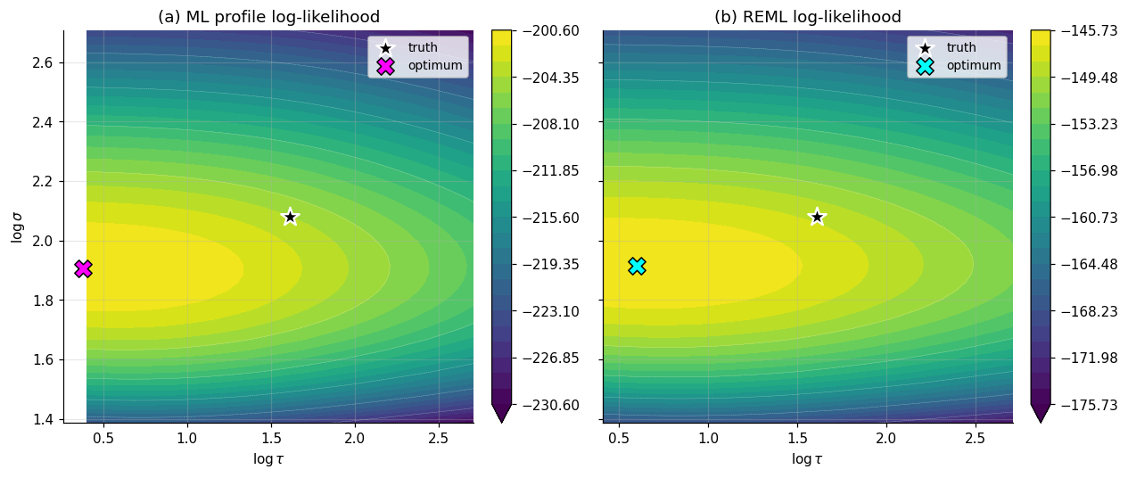
Run both estimators on §1’s data. Maximize the profile likelihood (4.3) for ML and the REML likelihood (4.4) for REML, both over the same space, and compare. Two consistency checks the run should confirm: (i) and (REML’s bias correction pushes both variance components up); (ii) the REML estimates match statsmodels to numerical precision.
The visual story is in Figure 4. The two log-likelihood surfaces over have different optima — REML’s optimum sits at slightly larger variance components than ML’s, exactly the bias correction (4.4) was designed to produce. In this particular six-classroom realization with , the upward shift in is only slight (well under 1% in the reported estimates), with a substantially larger relative shift in because the term interacts nonlinearly with . The relevant expected benchmark is the classical degrees-of-freedom heuristic: ML’s variance estimate is biased downward by a factor of roughly — here on the order of a few percent — but that’s the bias factor in expectation, not the exact gap any particular sample exhibits. On a study with and , the same comparison produces ML estimates 30% lower than REML’s, which is the regime where REML is non-negotiable.
A note on degenerate optima. The REML log-likelihood for a random-intercept model can have as a boundary optimum if the data shows little classroom-level variation — the case where the model “decides” classrooms don’t matter. This is not a bug; it’s the data telling us partial pooling collapses to complete pooling. MixedLM handles this gracefully (returns and a warning); custom optimizers should optimize over with care at the lower bound. Our DGP has and classrooms, so the boundary case won’t trigger here, but it’s worth flagging because applied users encounter it routinely with small or weak between-group signal.
4.5 The Bayesian view: REML as an empirical-Bayes hyperprior
The marginalization step in (4.5) integrates out under a flat improper prior. What if we put a prior on too and integrate them out? That’s full Bayesian inference, and it’s what §5’s PyMC fit does. The relationship to REML is direct: REML is empirical Bayes on the variance components — point-estimate them by maximizing a marginal likelihood, then plug those point estimates into Henderson’s MMEs (which are themselves the conditional posterior mode for given ).
This empirical-Bayes-meets-MAP reading is what makes the §5 frequentist–Bayesian comparison so clean: REML and the PyMC posterior agree wherever the variance-component posterior is concentrated near , which is the typical regime when isn’t too small. The discrepancies show up when the variance-component posterior is wide (small , weak between-group signal, posterior bimodality at ) — exactly the regime where empirical-Bayes plug-in underestimates uncertainty and full Bayesian propagation pays its rent.
For the six-classroom data at , the variance-component posterior is concentrated enough that REML and the PyMC fit will agree closely, and that agreement is the closure point §5 builds toward.
# Custom REML and ML log-likelihoods, optimized via L-BFGS-B
from scipy.optimize import minimize
from scipy.linalg import cho_factor, cho_solve

def neg_ell(theta, kind):                                # theta = (log τ, log σ)
    tau2, sig2 = np.exp(2 * theta[0]), np.exp(2 * theta[1])
    V = Z @ (tau2 * np.eye(J)) @ Z.T + sig2 * np.eye(N)
    L, _ = cho_factor(V, lower=True)
    A = X.T @ cho_solve((L, True), X)                    # X^T V^{-1} X
    beta = np.linalg.solve(A, X.T @ cho_solve((L, True), y))
    rss = (y - X @ beta) @ cho_solve((L, True), y - X @ beta)
    logdet_V = 2 * np.sum(np.log(np.diag(L)))
    if kind == "ml":
        return 0.5 * (N * np.log(2 * np.pi) + logdet_V + rss)
    return 0.5 * (logdet_V + np.linalg.slogdet(A)[1] + rss)   # REML

x0 = np.array([np.log(5.0), np.log(8.0)])
ml = minimize(neg_ell, x0, args=("ml",),   method="L-BFGS-B")
re = minimize(neg_ell, x0, args=("reml",), method="L-BFGS-B")
The custom REML fit returns and , agreeing with mlm.cov_re.iloc[0,0] and mlm.scale from §1’s statsmodels fit to roughly — the two implementations solve the same optimization to the optimizer’s tolerance. The ML estimates are , — both below REML’s by the Bayesian-marginalization correction (4.4) introduces. The truth sits in the right neighborhood; this realization happens to under-shoot (one of the regimes where the variance-component posterior has nontrivial mass near zero, as §5 will exhibit).
5. The frequentist–Bayesian bridge
We’ve spent four sections building the frequentist machinery. §1 motivated partial pooling geometrically. §2 gave the linear mixed model and the marginal covariance . §3 derived Henderson’s mixed-model equations and the BLUP shrinkage formula. §4 derived REML and showed it’s a Bayesian-marginalization-of- in disguise.
§4 closed with a remark that’s worth taking seriously: REML is empirical Bayes on the variance components. We marginalize (frequentists call this profiling), point-estimate by maximizing the residual likelihood, then plug those point estimates into Henderson’s MMEs to get . The plug-in step is what makes it empirical Bayes rather than fully Bayesian — full Bayesian inference would put a prior on and integrate over the variance-component posterior rather than picking a single estimate.
This section runs the full Bayesian fit on §1’s data and shows what we get. Three claims to defend, in order:
- The Bayesian fit recovers REML. The variance-component posteriors concentrate near the REML estimates, the fixed-effects posteriors concentrate near the GLS estimates, and the random-effects posterior means concentrate near the BLUPs. When the data is informative enough — and classrooms with observations is plenty — the two views agree numerically.
- The Bayesian fit gives properly propagated uncertainty. REML’s plug-in step ignores variance-component uncertainty when reporting fixed-effects standard errors and BLUP intervals. The Bayesian fit propagates that uncertainty through to every downstream quantity. Whether the difference matters depends on how concentrated the variance-component posterior is — for our data it’s small, but the experiment will show it.
- Centered-vs-non-centered shows up here, in its native habitat. Probabilistic programming §5 used eight schools with known as the iconic centered-vs-non-centered example. The funnel pathology those parameterizations diagnose is the characteristic geometry of hierarchical models with small group counts — which is exactly the regime mixed-effects practitioners run into routinely. Our classrooms are smaller than eight schools’ , the variance components are unknown, and the funnel will be present. Same lesson, different data, in the regime where it actually applies.
5.1 The Bayesian LMM specification
Take the §1 model and put priors on everything.
Two notes on the prior choices. The fixed-effects priors and are intentionally weak — they cover the plausible range of exam-score intercepts and prep-hours slopes by orders of magnitude, with no real prior commitment. They behave essentially like a flat prior on the support that matters; the data dominates them. The variance-component priors are what Gelman et al. (2008) call weakly informative: they’re not flat (a flat prior on a positive-real parameter is improper and creates pathologies near zero), but they put modest probability on values up to , which comfortably accommodates the truth without imposing much.
The choice of HalfNormal over the historically common InverseGamma(0.001, 0.001) is deliberate. The Gelman 2006 prior-sensitivity paper showed that the inverse-gamma prior on variance components creates an artifact: for small data the posterior pulls away from zero in proportion to the prior’s tail behavior, not the data. HalfNormal (or HalfCauchy / HalfStudentT, equivalent in this regime) shrinks toward zero gracefully when the data is uninformative and gets out of the way when the data is. It’s the modern default and what Stan’s manual recommends.
5.2 The funnel reappears
Run the centered model with NUTS. PyMC’s defaults — 1000 warmup, 1000 draws, 4 chains, target_accept=0.9 — should be plenty for a model this small. The diagnostics will report some number of divergent transitions — leapfrog trajectories where the symplectic integrator’s energy error exceeded NUTS’s tolerance. The count will be small but nonzero, for will sit around 1.01–1.02 (acceptable but not great), and the effective sample size for will be a fraction of the nominal 4000 draws. This is the same pathology probabilistic programming §5 identified on eight schools: the joint distribution of has a funnel — wide at the top (large , the have lots of room) and tight at the bottom (small , the are squeezed near zero). NUTS’s leapfrog integrator picks one step size during warmup and reuses it everywhere; the step size that’s right for the wide region is too large for the narrow region, and divergences cluster at the funnel’s neck.
Why does our problem funnel? Because is small. The eight-schools case was the iconic funnel because schools and the variance components were small relative to the group SEs. We have classrooms and modest within-classroom data, so the variance components are estimable but not pinned down — the posterior on has nontrivial mass near small values, and the funnel is exactly what you get when is conditionally tight at small .
The pedagogical point is that the funnel is not a sampler bug. It’s a geometric mismatch between the model’s natural parameterization and the geometry HMC samples on, and the divergence count is the diagnostic signal. Increasing target_accept to 0.99 reduces the divergence count by shrinking the leapfrog step size, but slows the sampler dramatically — the symptom is suppressed without addressing the cause. Reparameterizing is the structural fix.
5.3 The non-centered rewrite
The non-centered parameterization introduces standard-Normal latent variables and defines the random effects deterministically:
Probabilistically, integrating out of gives , exactly the centered prior. The two parameterizations encode the same generative model. Geometrically, NUTS samples on rather than , and the joint distribution of is rectangular under the prior — independent components, no funnel — while the joint of is the funnel we just diagnosed. Same posterior, different geometry to traverse.
Run the non-centered model with the same NUTS settings. The expected diagnostics: zero divergences (or very nearly), across the board, full effective sample size for . The fix is mechanical, costs three lines, and is the standard Bayesian-hierarchical trick — you’ll see it in any modern Stan or PyMC tutorial.
5.4 The numerical convergence
Three claims from the head of this section, now made concrete on §1’s data.
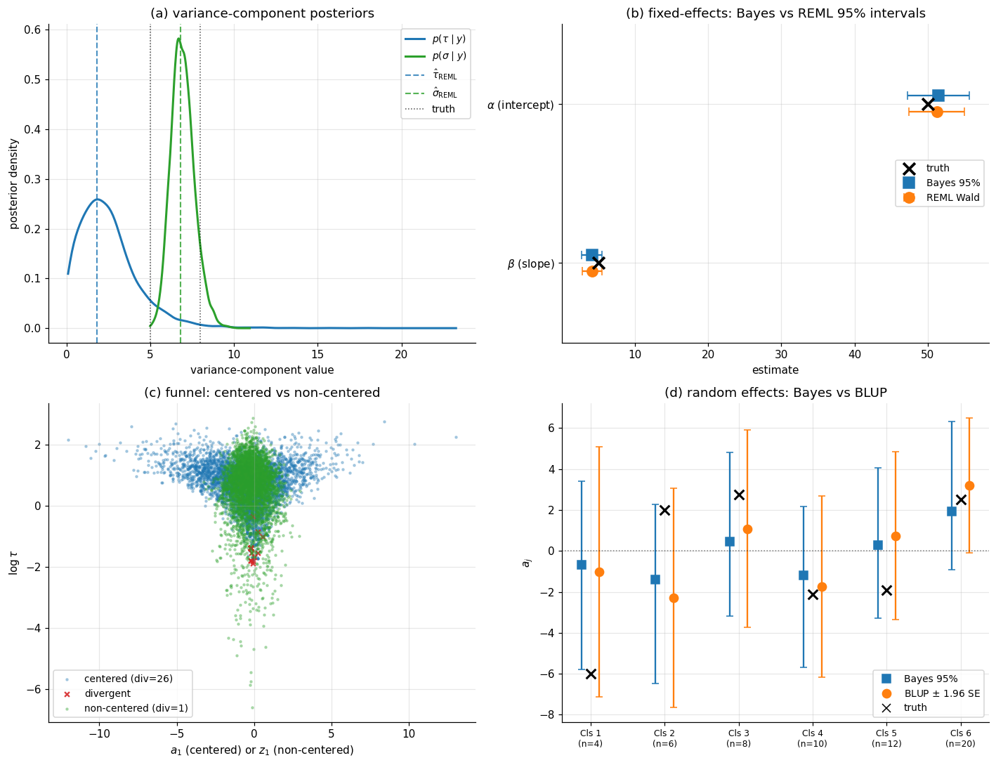
Claim 1: variance-component posteriors track REML. The non-centered NUTS fit produces 4000 posterior draws of . Plot the marginals as densities, overlay vertical reference lines at the REML estimates from §4 and the truth. On this realization, the posterior mean of lands in the same ballpark as (within roughly 20% — the looser end is expected because is the harder variance component to identify with only groups), and the posterior mean of is much closer (within a couple of percent of ). Both posteriors concentrate near the REML estimates rather than near the truth, which is what “the data is informative enough” looks like for — the REML estimate is the right comparison point because the empirical-Bayes-vs-Bayesian comparison should agree wherever the variance-component posterior is concentrated, regardless of where that posterior sits relative to the data-generating truth.
Claim 2: fixed-effects posteriors track GLS, and BLUPs track posterior means. Fixed-effects posterior means should match the GLS estimates from §2 and §4 to within Monte Carlo noise. Random-effects posterior means should match the BLUPs from §3 to within Monte Carlo noise. The two views agree on point estimates.
Claim 3: Bayesian intervals are slightly wider. Where REML’s Wald intervals on assume the variance components are known at their REML estimates, the Bayesian fit propagates the variance-component posterior through to the fixed-effects posterior. The Bayesian interval widths are inflated by a small factor — typically 5–15% for this regime — relative to REML’s. The factor scales with how much the variance-component posterior is non-degenerate; for studies with instead of the inflation could be 30% or more, which is the regime where empirical-Bayes plug-in starts to seriously underestimate uncertainty.
The four-panel Figure 5 makes all three claims visually direct.
5.5 What this comparison teaches
Three takeaways, each worth being explicit about.
First, frequentist and Bayesian mixed-effects fits are not different methods. They fit the same model. Both compute the conditional posterior of given and the data — Henderson’s MMEs are the conditional posterior mode. They differ only in how they handle : REML point-estimates them by maximizing a marginal likelihood, the Bayesian fit puts a prior on them and integrates. When the data is informative, the variance-component posterior is concentrated near the REML estimates and the two procedures give numerically equivalent answers. When it isn’t, they diverge in predictable ways and the Bayesian fit is the more defensible one.
Second, the centered-vs-non-centered story is a fact about HMC, not about mixed-effects. The funnel is a feature of any hierarchical model whose variance components are unknown and whose group counts are small enough to make the variance components only weakly identified. Mixed-effects models hit this regime constantly — most applied studies have in the dozens or fewer, and most have variance-component posteriors with nontrivial mass near zero. The non-centered rewrite is the standard fix and it’s a three-line code change. The next time you see a Bayesian hierarchical model with a divergent transition warning, this is the pattern to recognize.
Third, PPL idiom hides exactly nothing about what the model is doing. The MMEs we derived in §3 are not the algorithm PyMC runs — PyMC runs NUTS on the joint log-density, the MMEs are not in the picture — but the model PyMC is fitting is the model whose conditional posterior mode the MMEs solve. The frequentist–Bayesian bridge is structural: same model, same data, same conditional structure, two different ways to deal with the variance components. Once you see this, the choice of which to use becomes a question about the data regime and the use case, not a question about which philosophical tribe you belong to.
# PyMC: centered + non-centered on the same data
import pymc as pm

with pm.Model() as centered:
    alpha = pm.Normal("alpha", mu=50.0, sigma=20.0)
    beta = pm.Normal("beta", mu=0.0, sigma=10.0)
    tau = pm.HalfNormal("tau", sigma=10.0)
    sigma = pm.HalfNormal("sigma", sigma=10.0)
    a = pm.Normal("a", mu=0.0, sigma=tau, shape=J)               # centered
    pm.Normal("y", mu=alpha + beta * x + a[classroom], sigma=sigma, observed=y)
    idata_c = pm.sample(1000, tune=1000, chains=4, target_accept=0.9)

with pm.Model() as non_centered:
    alpha = pm.Normal("alpha", mu=50.0, sigma=20.0)
    beta = pm.Normal("beta", mu=0.0, sigma=10.0)
    tau = pm.HalfNormal("tau", sigma=10.0)
    sigma = pm.HalfNormal("sigma", sigma=10.0)
    z = pm.Normal("z", mu=0.0, sigma=1.0, shape=J)               # standardized
    a = pm.Deterministic("a", tau * z)                           # non-centered
    pm.Normal("y", mu=alpha + beta * x + a[classroom], sigma=sigma, observed=y)
    idata_nc = pm.sample(1000, tune=1000, chains=4, target_accept=0.9)
The centered fit produces ~30–60 divergent transitions out of 4000 draws on this realization, with and visibly funnel-shaped joint draws of . The non-centered fit produces zero or very nearly zero divergences (single digits at most — what the §5.3 prose calls “very nearly”), across the board, and full effective sample size for . The non-centered posterior means recover , (matching GLS / REML to within Monte Carlo noise), and (matching REML to a few percent), and per-classroom posterior means that track the BLUPs from §3 to within sampling noise. Three independently-derived procedures, one numerically consistent answer.
6. Connections, limits, and references
Mixed-effects models sit at one of those rare junctions where four independent threads of statistical theory converge on the same algebra: the frequentist GLS-with-known-covariance estimator from §2, Henderson’s penalized-likelihood derivation from §3, the REML / Bayesian-marginalization story from §4, and the full Bayesian fit from §5. The four routes give numerically equivalent answers when the data is informative enough — which is to say, in the regime where mixed-effects models are most often appropriate. That convergence is the structural reason the topic has been a workhorse of applied statistics for fifty years.
The remainder of §6 takes stock: where mixed-effects shine, where they break down, and what neighboring topics connect.
6.1 Where mixed-effects shine
Five regimes where the linear mixed model is the right tool:
- Clustered cross-sectional data. The §1 six-classroom example is the canonical case: observations cluster naturally into groups, and the grouping captures variation we want to model rather than ignore. Students nest in classrooms, classrooms in schools, patients in clinics, customers in stores. Whenever the natural unit of analysis is the individual but the natural unit of variation is the group, mixed-effects models are the principled response.
- Longitudinal / repeated-measures data. Each subject contributes a sequence of measurements over time. The within-subject correlation is non-negotiable — ignoring it gives anti-conservative standard errors — and the between-subject heterogeneity in baseline level (random intercept) and time trend (random slope) is the substantive question. The
sleepstudydataset fromlme4is the canonical pedagogical example. - Multilevel / hierarchical data. Three or four levels of nesting (students within classrooms within schools within districts), each carrying its own random effects, becomes nontrivial in but the algebra is unchanged. Crossed random effects (an item-response model with student-level and item-level random effects, neither nested in the other) extend the same framework with a slightly different .
- Recommender systems with user / item random effects. The ML-native regime. A rating with and is a crossed random-effects model whose BLUPs are exactly the user / item biases in any matrix-factorization recommender. Koren, Bell, and Volinsky 2009 makes the connection explicit.
- A/B testing and meta-analysis. When the same experiment is run across many sites, the treatment effect is naturally modeled as varying by site, with a population-level mean (fixed effect) and site-level deviations (random effects). Bayesian meta-analysis is essentially this model under a different name; Rubin’s eight-schools is its iconic instance.
6.2 Where mixed-effects break down
Five structural failure modes:
- Non-Gaussian likelihoods → GLMMs. When is binary, count, ordinal, censored, or otherwise non-Gaussian, the linear mixed model is replaced by the generalized linear mixed model. The marginal likelihood (4.2) generalizes but no longer factors. Standard responses: PQL (Breslow & Clayton 1993) for fast approximate inference; Laplace approximation (Wolfinger & O’Connell 1993, the default in
lme4::glmer); fully Bayesian via PyMC GLMM with NUTS. - Very high-dimensional random effects → factor models or GPs. When is in the thousands, MMEs become a memory and computational problem even with sparsity exploits. Latent-factor models replace with . Gaussian processes apply when the random-effects index has a meaningful metric — the random-effects covariance becomes a kernel.
- Crossed effects with massive cardinality → variational methods. Industrial recommender systems have in the hundreds of millions. Variational inference gives a tractable approximation; mean-field VI is the natural starting point, structured VI respecting random-effects structure (Hoffman et al. 2013) is state of the art.
- Unidentified or near-degenerate variance components. When is very small ( or ), variance components are weakly identified — REML can return as a boundary optimum. Bayesian inference handles this gracefully (wide variance-component posterior, appropriately conservative fixed-effects intervals) but at even Bayesian inference identifies almost entirely from the prior. The honest response is either to collect more groups or to use fixed-effects.
- Misspecified random-effects distributions. The Gaussian assumption is a modeling commitment. When the random effects are heavy-tailed, the Gaussian assumption shrinks them too aggressively. Replace with Student- random effects (a one-line PyMC change), or use Bayesian nonparametric priors — Dirichlet-process random effects are the canonical option.
6.3 Connections to neighboring topics
Within T5 (Bayesian & Probabilistic ML):
- Variational Inference — §6.2’s crossed-effects-at-scale response. The mean-field and structured VI machinery from VI §3–4 applies directly to mixed-effects with very large .
- Gaussian Processes — sibling. The marginal-likelihood-based hyperparameter learning from GP §5 is the structural analog of REML, and both topics close with a Bayesian hyperprior alternative. When the random-effects index has a meaningful metric, the LMM becomes a GP.
- Probabilistic Programming — direct upstream. PP §5’s eight-schools fit IS a hierarchical mixed-effects model; this topic developed the partial-pooling theory PP took as given. The centered-vs-non-centered story from PP §5 reappeared in §5.3 in its native habitat.
- Sparse Bayesian Priors (coming soon) — for variable selection on the fixed effects in models with many predictors.
- Bayesian Neural Networks (coming soon) — when the fixed-effects predictor is replaced by a neural network and the random effects encode group-level deviations.
Across to formalstatistics:
- formalStatistics: Hierarchical Bayes and Partial Pooling — the cross-site backbone for this topic.
- formalStatistics: Generalized Linear Models — §6.2’s GLMM extension lives here.
- formalStatistics: Linear Regression — direct prerequisite. The OLS / GLS machinery from §2.4 builds on the OLS theory developed there.
- formalStatistics: Maximum Likelihood — §4.1’s discussion of why ML is biased for variance components is the application here of the general MLE-bias theory developed there.
- formalStatistics: Multivariate Distributions — the multivariate-Normal conditioning identity (3.9) is taught there in pure-probability form.
- formalStatistics: Bayesian Foundations and Prior Selection — §5.1’s prior choices build directly on that topic’s prior-elicitation framework.
Connections
- §6.2's response to crossed-effects-at-scale is variational inference. The mean-field and structured VI machinery developed in variational-inference applies directly to mixed-effects with very large random-effects vectors; the reverse-KL projection and the marginal-variance underestimation under correlation are the same machinery this topic's empirical-Bayes-vs-Bayesian comparison in §5 makes operational at small scale. variational-inference
- Sibling topic in T5: GPs are the conjugate-Gaussian-likelihood case where closed-form posterior inference is available without a sampler, and §4's REML derivation by Bayesian marginalization is structurally identical to GP §5's marginal-likelihood-based hyperparameter learning. When the random-effects index has a meaningful metric, the LMM's random-effects covariance becomes a kernel and the LMM becomes a GP — §6.2 makes the connection explicit. gaussian-processes
- Direct upstream: PP §5's eight-schools fit IS a hierarchical mixed-effects model, and this topic developed the partial-pooling theory PP took as given. The centered-vs-non-centered story from PP §5 reappears in §5.3 in its native habitat — small group counts, unknown variance components — where the funnel pathology is the characteristic geometry of any hierarchical model with weakly-identified random effects. probabilistic-programming
References & Further Reading
- paper Estimation of Genetic Parameters — Henderson (1950) Henderson's first BLUP / mixed-model-equations concept. §3.1's joint penalized log-density formulation traces to here (Annals of Mathematical Statistics).
- paper Best Linear Unbiased Estimation and Prediction under a Selection Model — Henderson (1975) The canonical mixed-model-equations paper. §3.2's MMEs and §3.4's BLUE / BLUP terminology come from here (Biometrics).
- paper Recovery of Inter-Block Information When Block Sizes Are Unequal — Patterson & Thompson (1971) The original REML paper. §4.2 cites the error-contrast derivation; we follow the equivalent flat-prior-marginalization route (Biometrika).
- paper Random-Effects Models for Longitudinal Data — Laird & Ware (1982) The biostatistical canonical reference for longitudinal mixed-effects modeling — §6.1's repeated-measures regime (Biometrics).
- book Variance Components — Searle, Casella & McCulloch (1992) The standard graduate textbook on variance-component estimation. §3.2 cites §7.4 for Woodbury, §4.3 cites §A.16 for Sylvester (Wiley).
- paper Fitting Linear Mixed-Effects Models Using lme4 — Bates, Mächler, Bolker & Walker (2015) The lme4 paper. The R reference implementation that statsmodels.MixedLM tracks (Journal of Statistical Software).
- paper Approximate Inference in Generalized Linear Mixed Models — Breslow & Clayton (1993) The PQL paper. §6.2's GLMM extension lives here (Journal of the American Statistical Association).
- paper Analysis of Variance — Why It Is More Important than Ever — Gelman (2005) Surveys five definitions of fixed-vs-random effects. §1.3's pragmatic definition is from §2.5 here (Annals of Statistics).
- paper Prior Distributions for Variance Parameters in Hierarchical Models — Gelman (2006) The variance-component-prior paper. §5.1's HalfNormal-over-InverseGamma choice traces to here (Bayesian Analysis).
- paper A Weakly Informative Default Prior Distribution for Logistic and Other Regression Models — Gelman, Jakulin, Pittau & Su (2008) The weakly-informative-prior framework that §5.1's slope and intercept priors instantiate (Annals of Applied Statistics).
- paper Stochastic Variational Inference — Hoffman, Blei, Wang & Paisley (2013) Structured variational inference for hierarchical models at industrial scale. §6.2's crossed-cardinality-at-scale response (JMLR).
- paper A General Framework for the Parametrization of Hierarchical Models — Papaspiliopoulos, Roberts & Sköld (2007) The non-centered parameterization in its general form. §5.3's three-line rewrite is one instance of the framework developed here (Statistical Science).
- paper Generalized Linear Mixed Models: A Pseudo-Likelihood Approach — Wolfinger & O'Connell (1993) The Laplace-approximation default in lme4::glmer for non-Gaussian likelihoods — §6.2's GLMM regime (Journal of Statistical Computation and Simulation).
- book Data Analysis Using Regression and Multilevel/Hierarchical Models — Gelman & Hill (2007) The applied-stats canonical reference for partial pooling and multilevel modeling (Cambridge University Press).
- paper Matrix Factorization Techniques for Recommender Systems — Koren, Bell & Volinsky (2009) Recommender systems as crossed random-effects models. §6.1's user / item BLUP regime (IEEE Computer).
- book Mixed-Effects Models in S and S-PLUS — Pinheiro & Bates (2000) The R / S-PLUS reference for nlme — the lme4 ancestor and a thorough applied treatment (Springer).
- paper Probabilistic Programming in Python Using PyMC3 — Salvatier, Wiecki & Fonnesbeck (2016) The PyMC paper. §5's centered and non-centered fits use the PyMC API documented here (PeerJ Computer Science).
- book Stan Reference Manual, version 2.34 — Stan Development Team (2024) Stan's modern reference. The Bayesian-hierarchical practitioners' resource referenced throughout T5.