Variational Inference
Posterior approximation by reverse-KL projection onto a tractable family — the ELBO, mean-field CAVI, stochastic and reparameterization gradients, and normalizing-flow variational families
Overview
Bayesian inference begins with the same identity in every textbook:
The identity is conceptually clean: pick a prior, write a likelihood, divide. The catch is that for almost any model worth fitting, the integral defining has no closed form, and the right-hand side cannot even be evaluated without it.
The two scalable responses to this obstacle split the modern Bayesian computation literature in half. Markov chain Monte Carlo, the subject of Bayesian Computation and MCMC on formalstatistics, builds a Markov chain whose stationary distribution is the posterior and samples from it without ever computing — asymptotically exact at the cost of long chains and post-hoc convergence diagnostics. Variational inference, the subject of this topic, takes a different tack: pick a tractable family of distributions over , find the member closest to the posterior under some divergence, and report as the approximate posterior. VI is fast and deterministic. It is also approximate in a way MCMC isn’t, and the approximation error has a structure worth understanding before any algebra is on the page.
This topic develops the machinery in six sections. §1 frames the geometry — VI is a projection. §2 derives the evidence lower bound (ELBO), the algebraic device that makes reverse-KL projection tractable. §3 develops mean-field VI and CAVI on a Bayesian Gaussian mixture. §4 lifts both restrictions of §3 — full-batch and conjugate — through stochastic VI, the score-function gradient, the reparameterization gradient, and ADVI. §5 attacks the structural error of mean-field with full-rank Gaussian VI and normalizing flows. §6 closes with connections to the rest of the curriculum and the limits a working Bayesian needs to know about.
1. The intractable posterior
1.1 Why the evidence is intractable
A concrete example fixes the obstacle. Bayesian logistic regression takes data with covariates and binary responses , a parameter vector , and the likelihood
with a Gaussian prior on the regression coefficients. Up to the unknown evidence, the posterior is
which is log-concave in but not Gaussian: the term is not quadratic in , so the posterior is not in the same exponential family as the prior. Conjugacy fails. The marginal likelihood
has no analytic expression — the integrand is a product of logistic terms times a Gaussian, and no antiderivative reduces the -dimensional integral to closed form. Even evaluating at a single requires that integral.
The pattern generalizes. Conjugacy — the property that lets us write in closed form — is the exception, not the rule. Most models that lift a likelihood from a textbook example into a real application break conjugacy at some point: a logit link, a non-Gaussian noise model, a hierarchical structure with cross-level couplings, or a deep neural network whose weights play the role of . For all such models, the integral defining is the bottleneck.
1.2 Two responses: sampling versus optimization
MCMC sidesteps the intractable integral by exploiting a structural fact: ratios of the unnormalized posterior at two parameter values cancel the unknown exactly, so a Markov chain whose transition probabilities depend only on those ratios has the right stationary distribution. The chain runs, eventually mixes, and the post-mixing samples are drawn from the posterior. The cost is wall-clock time: a chain on a large model can take hours or days, and convergence diagnostics are part of every analysis.
Variational inference replaces the sampling problem with an optimization problem. We choose a variational family — a parametric set of distributions over — and search for the member of closest to the true posterior under a divergence :
The choice of controls expressiveness; the choice of controls what closest means. Once is in hand, posterior expectations are approximated by , which by construction is something we can compute. Both choices are deferred — to §3 and §5, to §1.3 below — but the bird’s-eye view is already informative: VI trades the exact-but-slow of MCMC for the approximate-but-fast of optimization, and the quality of the trade depends entirely on whether is rich enough to host a good approximation to the true posterior.
1.3 The geometric picture
Reading the optimization above out loud makes the geometry visible. The space of probability distributions on is some infinite-dimensional set; the true posterior is a point in that set; the family is a much smaller submanifold parametrized by some finite-dimensional vector ; and is the point on closest to the posterior under . Variational inference is a projection. When is too restrictive to contain the posterior, which is almost always the case, the projection introduces a bias, and the structure of that bias depends on what punishes most.
Two natural choices of give qualitatively different projections.
Forward KL, , takes the expectation under the true posterior:
Computing this expectation requires sampling from the posterior, which is exactly what VI is trying to avoid. So forward KL is a non-starter as a stand-alone VI objective — though it does appear in the literature, paired with sampling-based corrections (importance-weighted bounds, reweighted wake-sleep) that lie outside this topic.
Reverse KL, , takes the expectation under :
This is tractable in the sense that matters: is the distribution we chose, so we can sample from it (or compute expectations under it analytically when is in a simple family). The integrand involves , and the unknown constant separates cleanly from the parts that depend on — which is the entire point and the subject of §2.
Reverse KL is the standard VI objective, and it comes with a famous shape: the mode-seeking behavior previewed in KL divergence. A reverse-KL minimizer punishes mass placed where the target has none — where blows up the integrand — but pays no penalty for failing to cover regions where the target has mass and does not. When the target is multimodal, and the family is unimodal, the minimizer locks onto one mode rather than spreading across all of them. This is a feature in some applications (sharp predictions, decisive point estimates) and a pathology in others (genuine multimodality, identifiability problems where the modes correspond to distinct scientific hypotheses).
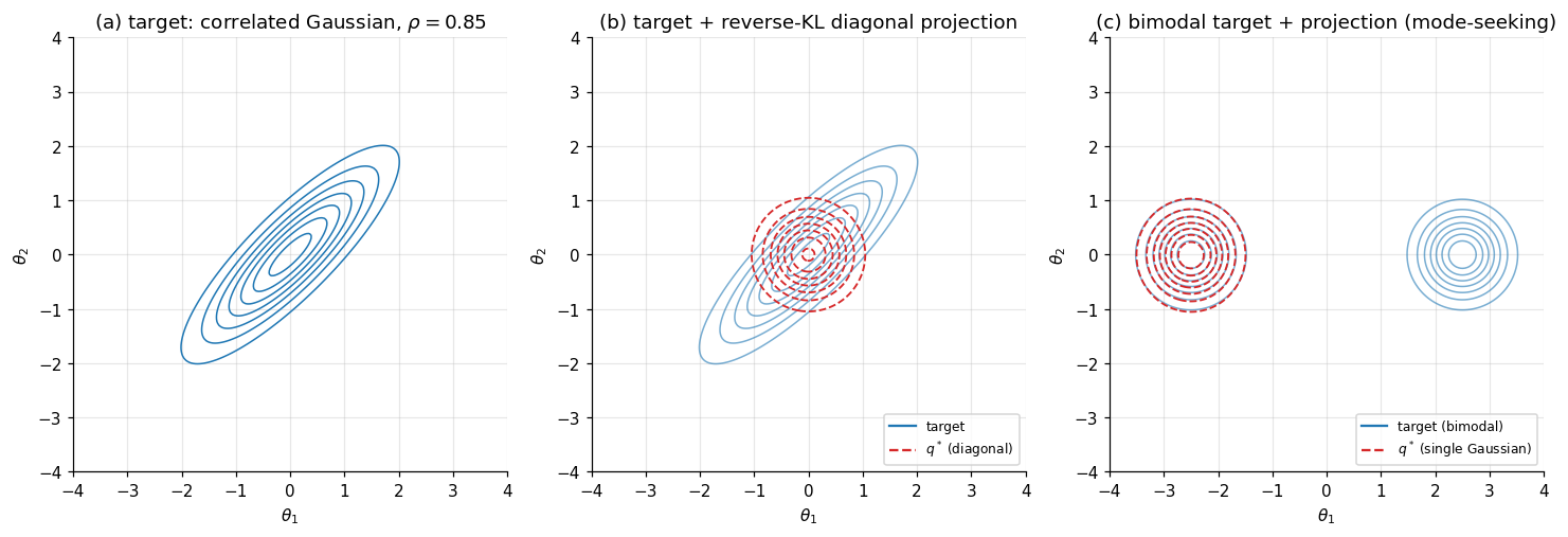
The figure below illustrates the geometry on two synthetic 2D targets. Panel (a) shows a posterior with off-diagonal correlation; panel (b) overlays the reverse-KL projection onto the mean-field family of diagonal Gaussians — the projection captures the center but cannot represent orientation, and (we will see in §3 and again in §5) systematically under-estimates the marginal variance along correlated directions. Panel (c) shows the mode-seeking pathology: a bimodal target on the left, the reverse-KL projection onto a single Gaussian on the right — locked onto one mode, with a symmetric solution at the other.
The §2 derivation makes the unknown disappear from the reverse-KL objective via an algebraic rearrangement called the evidence lower bound. With the ELBO in hand, §3 develops the workhorse mean-field algorithm, §4 extends VI to large-scale and non-conjugate problems, §5 lifts the mean-field assumption with structured families and normalizing flows, and §6 closes with connections and limits.
2. The ELBO
Reverse KL is tractable because is a distribution we chose; we can sample from it or compute expectations under it. But the integrand
still requires , and is the unknown evidence we cannot compute. The way out is an algebraic rearrangement that isolates as a constant — a constant from ‘s point of view, irrelevant to optimization. The rearranged objective is the evidence lower bound, or ELBO. Three properties make it the central object of variational inference: it is computable from the model and a sample from alone; it lower-bounds uniformly in ; and maximizing it over is equivalent to minimizing reverse KL to the posterior.
2.1 From Jensen to the ELBO
The derivation is a single application of Jensen’s inequality. Recall: a function is concave if for every integrable random variable . The natural logarithm is concave on , so for any positive random variable ,
Now the importance-sampling identity: for any density on that puts positive mass everywhere does,
The marginal likelihood is the expectation under of the ratio between the joint and . Taking logs and applying Jensen’s inequality to :
The right-hand side is the evidence lower bound. We give it a name and a notation.
Definition 1 (ELBO).
Let be a joint density on , a fixed observation, and a density on absolutely continuous with respect to — equivalently, wherever . The evidence lower bound of at is
with the convention .
Two properties are immediate from the derivation:
- for every admissible — Jensen’s inequality.
- is computable whenever the model’s joint density is computable and we can take expectations under . The unknown does not appear.
The first property explains the name: the ELBO is a lower bound on the evidence. The second explains why it matters: every quantity on the right-hand side is something we built and chose, so we can evaluate it.
2.2 The evidence decomposition
Jensen’s inequality tells us but not by how much. The gap turns out to have an exact, illuminating form.
Theorem 1 (Evidence decomposition).
For every admissible ,
Proof.
Start from the definition of reverse KL and substitute Bayes’ rule :
Expand the second term using :
where comes out of the expectation because it does not depend on . Substituting:
Rearranging gives the claim.
∎The decomposition is the operational identity of variational inference. Three consequences come immediately.
Maximizing the ELBO is equivalent to minimizing the reverse KL. Because does not depend on , it is a constant in the optimization over . So
The intractable optimization (reverse KL involves , which we cannot evaluate) and the tractable optimization (the ELBO involves , which we can) have the same argmax.
The bound is tight when contains the posterior. Reverse KL is non-negative and equals zero iff almost everywhere. So if the family is rich enough that , the optimum equals the posterior and . Outside the conjugate cases this almost never happens; the §3 mean-field GMM and §4 Bayesian logistic regression both have , and the gap measures the structural error of the family.
The ELBO is a free lower bound on the evidence. For model comparison or hyperparameter selection, is exactly the quantity we want to compare across models — a higher evidence is a better fit. Computing requires the intractable integral; the ELBO gives a lower bound that costs only a forward pass under . This is the substrate of Variational Bayes for Model Selection.
2.3 Three equivalent forms
Definition 1 gives one expression for the ELBO. Two algebraic rearrangements produce equivalent expressions, each useful in a different context.
Form 1: Energy plus entropy. The entropy of is . Substituting into Definition 1:
Reading: the ELBO rewards -mass in regions of high joint log-density (the energy term, by analogy with the Boltzmann distribution’s ) and rewards for being spread out (the entropy term). Maximizing the ELBO trades off between concentrating on the mode of and avoiding collapse to a delta. This form is canonical in the statistical-mechanics framing of VI as variational free-energy minimization — Feynman’s variational principle for the partition function, transcribed into Bayesian language.
Form 2: Reconstruction minus prior-KL. Decompose :
Reading: the ELBO rewards for placing mass on values that explain the data (the reconstruction term, ) but penalizes for moving away from the prior (the prior-KL term). This form is the workhorse of latent-variable models: in a variational autoencoder, the reconstruction term is the expected log-likelihood of the observed image given a latent code drawn from , and the prior-KL term keeps the encoder distribution close to the standard-Gaussian prior. The two terms encode the model’s bias-variance tradeoff at the level of .
Form 3: Evidence minus posterior-KL. This is Theorem 1 rearranged:
Reading: the ELBO equals the log-evidence (a constant) minus the reverse KL of to the posterior. This form makes the bound’s tightness transparent — the ELBO is closest to exactly when is closest to the posterior under reverse KL — and is the cleanest form for theoretical arguments. It is not directly useful for optimization, since the right-hand side contains the unknown and the unknown posterior.
The three forms are the same identity rearranged. Which one we reach for depends on what we want: Form 1 for thermodynamic intuition, Form 2 for implementation in latent-variable models, Form 3 for proofs.
2.4 Worked example: a conjugate Gaussian
A model with every quantity having a closed form lets us numerically verify the identity and visualize the ELBO landscape. We take the simplest such model.
Model. Observe with known. Place a Gaussian prior on the unknown mean. The joint density is
Exact posterior. Completing the square in inside gives the posterior in closed form:
where is the sample mean. The posterior precision is the prior precision plus times the data precision, and the posterior mean is the posterior precision times the data’s natural-parameter contribution. This is the standard Gaussian–Gaussian conjugate result.
Variational family. Take , the family of all 1D Gaussians. Crucially, the true posterior is in this family — the conjugate setup is the rare case where contains .
Closed-form ELBO. With , every expectation in Definition 1 has a closed form. We use the standard identity for any constant , plus :
Setting partial derivatives to zero recovers the exact posterior:
The variational optimum exactly equals the true posterior, as Theorem 1 predicted: when contains , the ELBO maximum saturates at and .
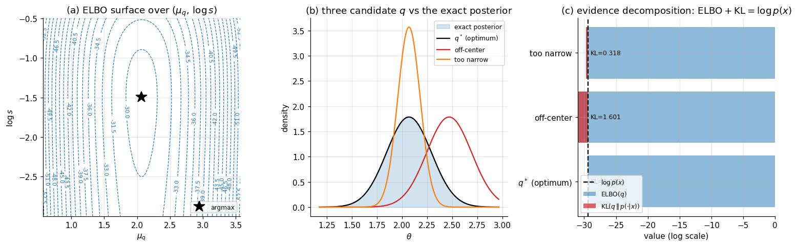
The figure below makes this concrete on a simulated dataset (, , , true ): panel (a) plots the ELBO surface over with the optimum marked, panel (b) overlays three candidate ‘s on the exact posterior (the optimum, an off-center version, and a too-narrow version), and panel (c) shows the evidence decomposition numerically — for each candidate, sits below by exactly , with the gap collapsing to zero at .
The conjugate case is not VI’s typical regime — most real models break conjugacy somewhere, and the §3 mean-field GMM is the first example where at the optimum. But the identity from Theorem 1 is universal: every ELBO maximization is a reverse-KL projection, and the gap to is always the KL of to the true posterior, whether that gap is zero or not.
3. Mean-field VI and CAVI
The §2 conjugate Gaussian example is misleading, because conjugacy is rare. For most Bayesian models, the posterior is not in the same family as the prior, the ELBO has no closed-form maximum even on simple parametric families, and Definition 1’s sole virtue is that it is an expression we can compute — not yet an algorithm we can execute. The mean-field assumption is the algorithmic move that turns the ELBO into something we can optimize coordinate-by-coordinate, and coordinate-ascent variational inference (CAVI) is the algorithm that results. CAVI is the workhorse of variational inference in conjugate exponential-family models — Bayesian Gaussian mixtures, latent Dirichlet allocation, factorial hidden Markov models, mixed-effects models, sparse linear regression with conjugate priors. The trade-off it makes is structural: mean-field cannot represent posterior correlations between variables in different blocks. §5 returns to that limit.
3.1 The mean-field family
Partition the latent variables into blocks: with . The blocks are arbitrary and chosen by the modeler — usually one block per parameter (fully factorized) or one block per logical group (e.g., all component means together, all assignments together).
Definition 2 (Mean-field variational family).
The mean-field family relative to the partition is
The factorization is across blocks; within a block, is unconstrained — any density on is admissible. So the family is simultaneously flexible (each can be any shape) and restrictive (the joint assumes block-independence).
What we gain is computational tractability. The ELBO under mean-field separates:
where the entropy term is a simple sum over blocks because under the factorization. The first term doesn’t separate — it depends jointly on all — but conditional on fixing every factor except one, it does, which is the door §3.2 walks through.
What we lose is correlation. If the true posterior couples and in different blocks (which it generically does — even simple regression posteriors couple the coefficient with the intercept), no can represent that coupling. The §1 panel (b) figure already showed this on a 2D Gaussian: the diagonal-Gaussian projection captures the center but cannot tilt to match the posterior’s correlated shape. §5 quantifies this loss as systematic under-estimation of marginal posterior variance along correlated directions.
3.2 The CAVI update
The optimization strategy for mean-field VI is coordinate ascent: cycle through the blocks , holding all factors except fixed and updating to its conditional optimum. The update has a clean closed form.
Theorem 2 (CAVI optimal coordinate update).
Fix . The unique maximizer of over densities on is
with the proportionality constant chosen to make a density.
Proof.
Hold fixed and write the ELBO as a functional of alone. Starting from Form 1 (energy plus entropy):
The last sum is constant in . For the first term, condition on and apply Fubini’s theorem:
where is the expected complete log-density viewed as a function of alone, with the expectation taken over the other factors. Substituting:
Define , with assumed finite. Then , and
So . The right-hand side is maximized over by minimizing the KL term, which is non-negative and equals zero iff almost everywhere. The unique maximizer is therefore .
∎The reading: the optimal given the others is proportional to the exponentiated expected complete log-joint, with the expectation taken over the other factors. This is also the form of the complete conditional as a function of — except with replaced by an expectation under . CAVI replaces conditioning on a value with averaging over a distribution.
Algorithm (CAVI). Initialize . Repeat until convergence:
- For : set .
Convergence is monitored by tracking the ELBO; halt when the ELBO change between sweeps falls below a tolerance.
The monotonicity of the ELBO under CAVI follows immediately from Theorem 2: each block update either increases the ELBO (if wasn’t already optimal) or leaves it unchanged, so the ELBO is non-decreasing across iterations. Like EM, CAVI is guaranteed to converge to a local maximum of the ELBO; the global maximum is generally unattainable because the ELBO is non-concave in for non-trivial models — particularly for mixtures, where the symmetry across component labels generates exponentially many local maxima.
3.3 Conjugate exponential families
CAVI’s update has a closed form whenever the model is conditionally conjugate — meaning each complete conditional is in an exponential family. The derivation is short, and the result is operationally important.
Suppose
with base measure , sufficient statistics , natural parameter , and log-partition . The exponential-family form means the dependence on enters only through and , while the dependence on the rest enters only through and .
Writing and noting that the second term is constant in :
Exponentiating gives the CAVI update:
This is in the same exponential family as , with natural parameter .
Proposition 1 (Conjugate CAVI in closed form).
If the complete conditional is in an exponential family with natural parameter , the CAVI update sets to the same exponential family with natural parameter .
The result is “expectation inside the natural parameter”: take the natural-parameter expression for the complete conditional, and replace each occurrence of with the appropriate expectation under . The class of conditionally conjugate models — where every complete conditional is an exponential family with a tractable expectation — is the natural domain of closed-form CAVI: Bayesian GMMs, LDA, hidden Markov models, factorial HMMs, and the broader family of conjugate hierarchical models that defines structured Bayesian-machine-learning workflows.
3.4 Worked example: Bayesian Gaussian mixture model
The canonical worked example is the Bayesian Gaussian mixture. We take the simplest version that exhibits all the structure: known component variance, a Gaussian prior on component means, and uniform mixing weights.
Model. Observe . Place a -component mixture with:
- Component means for ;
- Cluster assignments (uniform mixing weights);
- Observations with known.
The latent variables are with and .
Mean-field family. Take a two-block factorization: one block for the means, one for the assignments.
The within-block factorizations across and are part of the mean-field choice rather than implied by the generative model — in general, within-block posterior dependencies can remain — but for this conjugate GMM the §3.3 expectation-inside-the-natural-parameter argument makes them optimal at the CAVI fixed point: given the other block, the complete conditionals factor cleanly across for and across for , so writing the factorizations down loses nothing here.
The CAVI updates. Both updates follow from the conjugate exponential-family setup of §3.3.
Update for . The complete conditional depends only on and . It’s categorical with . The natural parameter has term . Taking the expectation under and using gives the responsibility:
normalized so . The variance-correction term softens the responsibilities relative to the EM hard-assignment limit: posterior uncertainty about pulls the soft assignments toward uniformity.
Update for . The complete conditional is a Gaussian — conjugate combination of the prior and the points hard-assigned to component . Replacing the hard assignments with expected responsibilities under gives the §2 conjugate Gaussian–Gaussian update applied to soft-assigned sufficient statistics:
where is the effective count of points assigned to component . Compare with §2: the only change is that the data is weighted by responsibilities rather than counted indicator-by-indicator. The connection to EM is now visible — CAVI’s -update is the soft E-step, and CAVI’s -update is a Bayesian M-step that returns the full posterior rather than just the MAP point.
The closed-form ELBO. Every term of has a closed form. Working through and the entropies:
where , , and the constant absorbs the data-independent normalizers. Tracking this expression across CAVI sweeps is the §3.4 figure.
The figure below shows CAVI applied to a synthetic 2D 2-cluster dataset designed to mirror the structure of Old Faithful eruptions (two well-separated clusters with moderate within-cluster spread). Panel (a) shows the data with a random initialization of component means; panel (b) shows the converged variational posterior, with each at its cluster center and the variational covariance as a 2-sigma ellipse; panel (c) shows the ELBO across iterations.
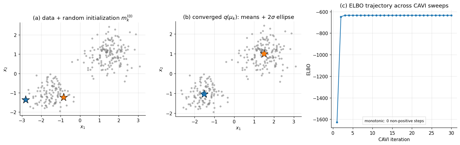
The convergence pattern is characteristic of CAVI on mixtures: the ELBO climbs rapidly in the first few sweeps as the responsibilities sort the points, then plateaus as the component means refine. Mixture posteriors are multimodal — any permutation of the component labels gives an equivalent posterior, and CAVI converges to one of those modes. §5 returns to the consequence that under mean-field, the component-mean variances are systematically smaller than under the full Bayesian posterior, because the mean-field assumption ignores the posterior coupling between and .
4. Stochastic and black-box VI
The CAVI setup of §3 — closed-form coordinate updates derived from conjugate-exponential-family structure — is the right tool for a specific class of models, and a wrong tool everywhere else. Two stresses that modern Bayesian workflows routinely encounter break it. The first is scale: when the dataset is large enough that even a single full-batch pass is expensive, the linear-in- cost of every CAVI sweep makes the method impractical. The second is non-conjugacy: when the likelihood and prior do not align in a way that produces closed-form complete conditionals, §3.3’s “expectation inside the natural parameter” trick has nothing to operate on, and the CAVI update has no analytic form.
This section assembles the two responses. Stochastic variational inference (Hoffman et al. 2013) addresses scale by computing CAVI updates from minibatches under a Robbins–Monro step-size schedule. Black-box variational inference (Ranganath, Gerrish, and Blei 2014) and the reparameterization gradient (Kingma and Welling 2014; Rezende, Mohamed, and Wierstra 2014) address non-conjugacy by recasting ELBO maximization as stochastic gradient ascent on a parametric variational family — and the reparameterization gradient is now the dominant computational device of modern VI, the substrate of every variational autoencoder, Bayesian neural network, and deep generative model. The §4.5 worked example applies the reparameterization gradient to Bayesian logistic regression on the Iris dataset using JAX.
4.1 Where CAVI breaks
Big data. A CAVI sweep on the §3 worked example — , , — costs roughly floating-point operations per iteration. For the corpus-scale topic models that motivated SVI ( documents, topics, vocabulary terms), the same scaling produces operations per sweep, and convergence can require hundreds of sweeps. The cost is not in any single update — each update is closed-form — but in the linear-in- scaling of every CAVI iteration. Wall-clock time runs to hours or days before the first ELBO estimate stabilizes. The standard remedy in optimization is to replace full-batch gradients with unbiased minibatch estimates and to rely on stochastic approximation theory for convergence. The §4.2 SVI machinery transfers that idea to CAVI’s natural-gradient form.
Non-conjugacy. Bayesian logistic regression is the simplest example. With Bernoulli likelihood and Gaussian prior , the complete log-joint is
which is not in the same exponential family as the prior — the term is not quadratic in . Mean-field CAVI on a Gaussian variational family would require in closed form, and that expectation has no analytic expression. Model-specific workarounds exist — local-variational bounds (Jaakkola and Jordan 2000), Laplace-style expansions around the variational mean — but each non-conjugate likelihood needs its own analysis, and no general recipe scales across the modeling landscape. The §§4.3–4.4 black-box machinery is general: any model where we can evaluate at a sampled admits a stochastic gradient estimator for the ELBO.
4.2 Stochastic VI for big data
Hoffman, Blei, Wang, and Paisley (2013) extended CAVI to the minibatch regime through two observations: that CAVI’s coordinate update is a natural gradient step on the ELBO, and that natural gradients in conditionally conjugate models admit unbiased minibatch estimators.
The natural gradient takes seriously that lives on a manifold of probability distributions rather than in the Euclidean space of natural parameters. The Euclidean gradient asks how the ELBO changes as moves a unit step in coordinate space; the natural gradient , where is the Fisher information of , asks how the ELBO changes as moves a unit step in KL distance. The natural gradient is the right object whenever the parameter space’s Euclidean geometry is misleading — which it always is for probability distributions.
Proposition 2 (Hoffman et al. 2013).
For a conditionally conjugate exponential-family model, with mean-field in the same exponential family as the complete conditional and the natural parameter of , the natural gradient of the ELBO with respect to (holding fixed) is
The result is operationally direct: the natural gradient points from the current natural parameter to the CAVI target. A natural-gradient ascent step with rate is a damped CAVI update,
and CAVI itself is the special case — a one-shot natural-gradient step that overshoots a damped trajectory but converges at every iteration.
The minibatching step is now mechanical. The CAVI target in conjugate exponential-family models has the form where is the prior natural parameter and is a per-datapoint sufficient-statistic contribution. Replacing the full sum with a rescaled minibatch sum,
gives an unbiased estimator of the CAVI target. Stochastic natural-gradient ascent with this estimator and a Robbins–Monro learning-rate schedule (, , typically for ) converges to a local maximum of the ELBO. SVI scales the workhorse CAVI machinery from research-scale to corpus-scale models — LDA on Wikipedia-sized corpora, hierarchical Dirichlet processes on millions of documents, factorial hidden Markov models on long time series — and remains the right tool for any conjugate exponential-family model that doesn’t fit in memory. It is not the right tool for non-conjugate models, where the natural gradient itself is not closed-form.
4.3 Black-box VI: the score-function gradient
For non-conjugate models, we need a gradient estimator that requires only the ability to (i) sample from and (ii) evaluate at a sampled . Ranganath, Gerrish, and Blei (2014) showed that the log-derivative trick — also known as the REINFORCE estimator in reinforcement learning (Williams 1992) and the likelihood-ratio estimator in stochastic optimization — provides exactly this.
Let be a parametric variational family with parameters , and write .
Theorem 3 (Score-function gradient).
Assume is differentiable in for each and that the dominated-convergence conditions hold. Then
Proof.
Differentiate under the integral sign, apply (the log-derivative trick), and split the result into two pieces:
The first term, after substituting , equals . The second term equals , the standard identity that the expected score is zero. So only the first term survives.
∎The estimator is universal in a clean sense: it requires only that we can sample from and evaluate both and . The model can be arbitrarily non-conjugate, hierarchical, deep — the score-function gradient still applies. Replacing the expectation with Monte Carlo samples gives the unbiased estimator
Universality has a cost. The estimator’s variance scales with the variance of the integrand under , and that variance is large whenever the variational distribution is far from the posterior — exactly the regime we expect at the start of optimization. Variance-reduction techniques (control variates, Rao–Blackwellization, the “score-function with baselines” recipe of Ranganath et al.) reduce practical variance by one to two orders of magnitude, but a comparison with the §4.4 reparameterization estimator still typically favors reparameterization when available. The score-function gradient remains the right tool for discrete variational families (where reparameterization fails because gradients cannot pass through a sampling-from-discrete operation) and is the gradient estimator under the hood of Pyro’s TraceGraph_ELBO and similar discrete-VI implementations.
4.4 The reparameterization gradient and ADVI
When the variational family admits a differentiable sampling path — when we can write with drawn from a fixed base distribution that does not depend on — there is a much lower-variance gradient estimator. The canonical example: with admits the sampling path
For any , the right-hand side has the right distribution, and the dependence on is through rather than through .
Theorem 4 (Reparameterization (pathwise) gradient).
Suppose with (independent of ), , differentiable in for each , and a function such that . Then
Proof.
By the change-of-variables theorem and independence of from ,
The right-hand side has only inside , not in the measure. Differentiating under the integral sign — the dominated-convergence integrability assumption is what licenses this — gives .
∎Applied to the ELBO with and the Gaussian reparameterization :
and the chain rule unpacks . The score-function estimator weights the value against the score ; the reparameterization estimator passes the gradient through the model itself. Empirically, the second has variance one to several orders of magnitude lower than the first for typical neural-network and conjugate-Gaussian targets — the sample-by-sample variance of is much larger than the variance of its gradient. The §4.5 worked example renders the variance comparison numerically.
ADVI: automatic differentiation variational inference. Kucukelbir, Tran, Ranganath, Gelman, and Blei (2017) packaged the reparameterization gradient into a recipe that applies automatically to any model expressible in a probabilistic programming language. The recipe has three ingredients:
- Constrained-to-unconstrained transform. Many parameters live on constrained manifolds — variances , simplex weights , correlation matrices in . Apply a smooth bijection that maps the constrained space to (log for positive reals, stick-breaking for the simplex, the Cholesky-correlation transform for correlation matrices). Bayesian inference on the unconstrained space adds a Jacobian correction to the log-prior.
- Variational family on the unconstrained space. The default is mean-field Gaussian, in unconstrained coordinates ; full-rank Gaussian, with a lower-triangular Cholesky factor, is the immediate generalization.
- Reparameterization gradient + autodiff. The ELBO’s gradient is computed via Theorem 4, with supplied by automatic differentiation through the model.
ADVI is what is under the hood of Stan’s advi, PyMC’s fit(method='advi'), NumPyro’s SVI with Trace_ELBO, and Pyro’s variational machinery. The §4.5 example is essentially a hand-rolled ADVI implementation in JAX — a five-line variational family, -line training loop — that produces the same gradients these frameworks compute internally.
4.5 Worked example: Bayesian logistic regression
We close §4 with reparameterization-gradient VI for Bayesian logistic regression on the Iris versicolor-vs-virginica classification problem (, features: petal length and petal width, plus a bias term). The model is
with a weak Gaussian prior. The variational family is mean-field Gaussian, , parametrized by , with reparameterization , .
The implementation has three pieces. The MC ELBO is the negated training objective, evaluated with Monte Carlo samples per gradient step. The reparameterization gradient is jax.grad of the MC ELBO with respect to ; JAX’s autodiff handles the chain rule through and through the model’s log-joint without any manual derivative work. The training loop runs 1000 Adam steps with learning rate 0.05; convergence is tracked through the MC ELBO, which fluctuates from sample to sample but trends upward and stabilizes after a few hundred iterations.
We benchmark against a Laplace approximation: find the MAP by gradient ascent on the log-posterior, then approximate the posterior as . On a log-concave posterior with data points, Laplace is sharp enough to serve as a reference for the variational marginals. (HMC would be sharper and is the canonical reference; we use Laplace here for runtime — HMC on Bayesian logistic regression takes much longer than the 60-second §4 budget allows.)
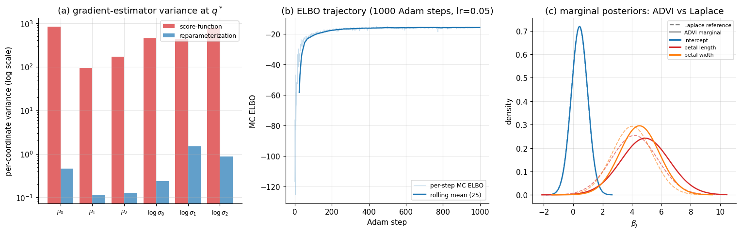
The §4 figure has three panels. Panel (a) compares the per-coordinate gradient variance of the score-function estimator and the reparameterization estimator at the converged variational parameters; the reparameterization estimator’s variance is typically one to two orders of magnitude lower. Panel (b) shows the MC ELBO trajectory across the 1000 Adam steps. Panel (c) overlays the marginal variational densities for on the Laplace marginals, showing that ADVI’s mean-field Gaussian recovers the marginal locations and approximate scales of the Laplace reference even though the underlying posterior has off-diagonal correlation that mean-field cannot represent. (§5 returns to that residual error.)
5. Beyond mean-field: structured VI and normalizing flows
The §3–§4 machinery treats every block of the variational factorization as independent of every other block. That structural assumption pays off in algorithmic simplicity — closed-form CAVI updates, separable ELBO entropies, single-coordinate gradient steps — and costs us in approximation quality whenever the true posterior has correlation structure that the factorization throws away. This section quantifies the cost (§5.1), introduces the immediate fix (§5.2), develops the rich-family approach via normalizing flows (§5.3), and runs all three approaches on a 2D banana-shaped target where the mean-field assumption is visibly inadequate (§5.4).
5.1 The structural error of mean-field
The cleanest demonstration of mean-field’s structural error is a closed-form result on Gaussian targets. The statement says: when we project a correlated multivariate Gaussian onto its mean-field family under reverse KL, every marginal variance comes out at most as large as the true marginal — strictly smaller when the corresponding coordinate is correlated with the others.
Theorem 5 (Mean-field underestimates marginal variance — Gaussian case).
Let on with positive definite, and let be the mean-field Gaussian family. The reverse-KL projection has and
with equality if and only if is independent of under .
Proof.
Write . The KL divergence between two zero-mean Gaussians is
The dependence on is through the positive-definite quadratic , minimized at . Substituting and using and :
Setting :
which is the precision-matched factorization. To see that , partition around index as , with the scalar diagonal entry, a row, and the submatrix obtained by deleting row and column . The Schur complement gives the -th diagonal entry of the inverse:
so
Because is positive definite, so is its principal submatrix , hence is positive definite, hence the quadratic form , with equality iff . The latter condition is exactly , equivalent to under the joint Gaussian.
∎The reading: when we coerce a correlated Gaussian into a product of independent Gaussian marginals, each marginal variance shrinks from (the true marginal) to (the conditional variance of given at zero, since for a Gaussian ). Mean-field VI confuses the marginal with the conditional, and the conditional is always tighter.
The §1 panel (b) figure was a special case of this theorem: a 2D Gaussian with correlation , where the diagonal-Gaussian projection shrinks each marginal variance by a factor of . The §3 GMM and §4 logistic-regression posteriors are not Gaussian, so Theorem 5 doesn’t apply literally; but the qualitative phenomenon — mean-field VI’s reverse-KL projection systematically underestimates posterior uncertainty along correlated directions — extends to general posteriors with empirical regularity (Turner and Sahani 2011), without admitting a comparably clean closed form.
The consequence for downstream inference is operational: a credible interval read off a mean-field posterior is narrower than the corresponding interval from MCMC, often by a factor large enough to materially change conclusions about whether a parameter is “significantly” different from zero. The §5.4 banana experiment makes this visible at scale, and §6 returns to it as one of VI’s headline limitations.
5.2 Full-rank Gaussian VI
The simplest fix lifts the mean-field constraint while keeping the variational family parametric. Replace
where is lower triangular (the Cholesky factor of the variational covariance), parametrized so its diagonal is positive — the standard recipe is for unconstrained . The full-rank family is the broadest Gaussian variational family: it can represent any Gaussian distribution on , including all correlation structures.
The §4 reparameterization recipe extends without modification. The sampling path is with , and the log-density is
with from the triangular form. The ELBO gradient is jax.grad of the MC ELBO; nothing changes. The cost is the parameter count: rather than , which is fine for moderate (hundreds) and prohibitive for high-dimensional latent spaces (millions, as in deep generative models). For Bayesian models with up to thousands of parameters — Bayesian logistic regression, Gaussian processes, mixed-effects models with moderate random-effect dimension — full-rank ADVI is the reasonable default, and Stan, PyMC, and NumPyro all expose it as a one-line option.
When the true posterior is approximately Gaussian — for instance, when the Bernstein–von Mises theorem applies, and is large enough that the posterior concentrates around the MLE — full-rank VI exactly recovers the right covariance. The Laplace approximation in §4.5 is the special case where the variational mean is fixed at the MAP, and the variational covariance is fixed at the inverse-Hessian; full-rank VI jointly optimizes both and produces the same answer in the large- limit, sometimes with better small- behavior because the variational objective is global rather than local.
When the true posterior is not approximately Gaussian — multimodal, banana-shaped, funnel-shaped, heavy-tailed — even full-rank Gaussian fails, because no Gaussian can curve, branch, or split. The §5.4 banana posterior is the canonical visual demonstration; the §5.3 normalizing-flow machinery is the response.
5.3 Normalizing flows
A normalizing flow is a parametric family of invertible, differentiable maps . Composed with a tractable base distribution on (typically standard Gaussian), it produces a variational distribution on whose density is given by the change-of-variable formula.
Definition 3 (Normalizing-flow variational family).
Let be a fixed density on and a parametric family of invertible, maps with Jacobian . The normalizing-flow family is
with density
For VI, we never need to evaluate at an arbitrary . The reparameterization recipe — sample , push forward to , evaluate at this — gives
which only requires the forward Jacobian determinant, never the inverse map. The ELBO under a flow variational family is
and the reparameterization gradient (Theorem 4) applies directly: differentiate with respect to , sum over MC samples, and ascend with Adam.
The whole game in flow design is the Jacobian determinant. A general has a dense Jacobian whose determinant costs to compute — prohibitive for any non-trivial . Productive flow architectures engineer so is triangular, diagonal, or otherwise cheap.
Coupling layers (Dinh, Sohl-Dickstein, and Bengio 2017, “Real NVP”). Split the input into two halves, . Define
where are arbitrary neural networks (no invertibility constraint required, since they appear only as multiplicative scale and additive shift). The Jacobian is block-triangular:
so — linear in . Stacking coupling layers with alternating partitions (where each half passes through) gives a flexible flow with a cumulative Jacobian that remains linear in per evaluation.
Autoregressive flows (Kingma, Salimans, Jozefowicz et al. 2016, “IAF”; Papamakarios, Pavlakou, and Murray 2017, “MAF”). Each output coordinate depends only on the previous ones: . The Jacobian is triangular by construction. IAF runs the autoregressive direction forward (cheap to sample, expensive to evaluate density at arbitrary , fine for VI, which only needs the forward direction); MAF runs it backward (cheap density evaluation, expensive sampling, better suited to density estimation).
Continuous-time flows (Chen et al. 2018, “Neural ODEs”), residual flows, and spline flows further extend the toolkit. The complete taxonomy of normalizing-flow architectures, their invertibility classes, and their tradeoffs is the subject of the planned Normalizing Flows (coming soon) topic in T3; we treat them here only as a variational family and forward-link for the architectural detail.
5.4 Worked example: a banana posterior
A clean visual demonstration of all three families pits them against a 2D non-Gaussian target with strong nonlinear dependence. We take the target
which produces a banana-shaped density curving downward — the canonical hard target for VI demos because (i) it is non-Gaussian, (ii) it has strong nonlinear dependence between and , and (iii) it is unimodal, so the failure modes are about shape rather than mode collapse.
We fit three variational families to this target by reparameterization-gradient ascent on the (unnormalized) ELBO with Adam:
- Mean-field Gaussian: , four parameters.
- Full-rank Gaussian: with lower-triangular , five parameters.
- Normalizing flow: four alternating coupling layers, each with a small MLP ( for the scale-and-shift), about 130 parameters.
The §5 figure has four panels in a 2×2 layout. Panels (a)–(c) show samples from each fitted variational distribution overlaid on contours of the target. The reader should see: (a) mean-field samples scattered as an axis-aligned isotropic blob, missing the curvature entirely; (b) full-rank samples forming a tilted ellipse that captures the linear correlation but cannot bend; (c) flow samples tracing the banana’s curve. Panel (d) shows the ELBO trajectories on a common axis: the flow’s ELBO climbs higher than full-rank, which climbs higher than mean-field. Since the target is normalized, all three ELBOs are bounded above by zero, and the gap from zero at convergence equals the residual KL between the fitted and the target — a direct read-out of how much structural error each family carries.
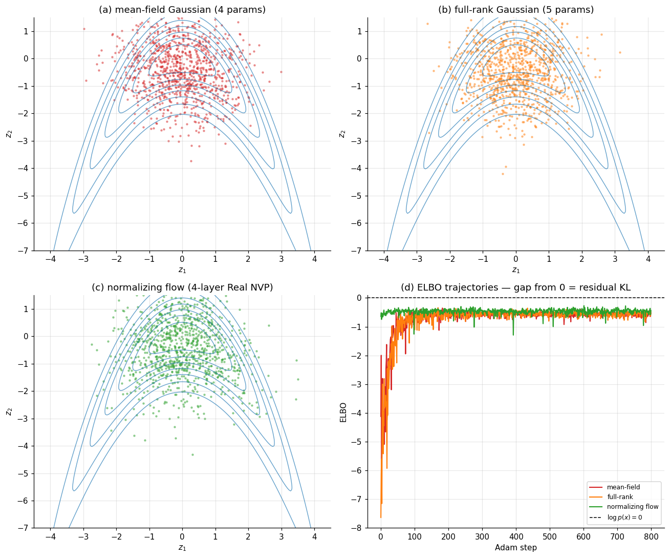
The flow’s gain is qualitative: it can represent the curve. The full-rank vs. mean-field gap is quantitative — the linear correlation full-rank captures and mean-field misses. Both kinds of structural error are recovered by Theorem 5’s mechanism: the mean-field family has too few degrees of freedom to track the target’s geometry, and the residual KL measures exactly how much.
6. Connections and limits
Variational inference sits at a junction. Backward, it inherits the divergence machinery developed in KL divergence and the Bayesian-computation framing developed across the formalstatistics Bayes track. Forward, it is the substrate of half a dozen planned T5 topics — Bayesian neural networks, normalizing flows as standalone density estimators, probabilistic programming, sparse Bayesian priors, meta-learning, and variational Bayes for model selection. Sideways, it shares deep structural ties with optimization (the ELBO is a free-energy minimization), with information theory (Fano-type lower bounds appear in mutual-information VI), and with the geometry of probability distributions (the natural gradient of §4.2 is the Fisher metric on the space of ). This section orients the topic among its neighbors, then lays out the assumptions and pathologies that bound where VI is the right tool and where it isn’t.
6.1 Within formalML
KL divergence. The substrate. The reverse-KL projection that defines VI’s optimization target, the mode-seeking versus mode-covering asymmetry that explains §1’s pathological collapse on multimodal targets, and the variational representations of f-divergences that underpin discriminator-based VI variants — all of it lives in the kl-divergence topic. Readers arriving at VI without that background should expect Theorem 1’s evidence decomposition to feel less natural than it should.
Convex analysis. The ELBO is concave in on its full support (the space of all distributions absolutely continuous with respect to ) — a consequence of KL’s joint convexity in its arguments. On parametric variational families, the concavity in is generally lost, which is why §3.4’s mixture-model CAVI converges only locally and why every §4 example uses Adam rather than a Newton-style global solver. The machinery of convex analysis — Fenchel duality, the Bregman-divergence framing of mirror descent — is what gives §4.2 natural gradient its theoretical grounding (mirror descent on the negative entropy is exactly natural-gradient ascent on the parametric family).
Gradient descent. The §4 black-box and reparameterization estimators all feed into stochastic gradient ascent, and every convergence guarantee available for VI is a convergence guarantee for SGD on a particular (generically non-convex) objective. The Robbins–Monro step-size schedule under which §4.2’s stochastic VI is consistent is the same one that underlies SGD for convex stochastic objectives.
Information geometry. The natural gradient of §4.2 is the gradient on the statistical manifold of , with the Fisher information as the metric tensor. Information-geometric perspectives also clarify why mean-field VI’s structural error from §5.1 is intrinsic, not algorithmic: the mean-field family is a low-dimensional submanifold of the full distribution space, and the reverse-KL projection onto it is the orthogonal projection in the Fisher–Rao metric, with all the rigidity that orthogonal projection implies.
Forward links to planned T5 topics. VI is the substrate, in different ways, of:
- Bayesian Neural Networks. Mean-field weight-space VI is the original recipe (Hinton and van Camp 1993; Graves 2011; Blundell et al. 2015); the §4.4 reparameterization gradient makes it tractable for deep networks. The structural-error theorem of §5.1 motivates the modern shift toward more expressive variational posteriors (full-rank in lower dimensions, normalizing flows in higher dimensions).
- Normalizing Flows (coming soon). §5.3 introduced flows as a variational family. The dedicated topic develops them as standalone density estimators, develops the full architectural taxonomy (coupling, autoregressive, continuous-time, residual, spline), and treats the inverse direction — flows for sampling from data distributions in deep generative modeling.
- Probabilistic Programming (coming soon). Stan, PyMC, and NumPyro all expose ADVI as a one-line option; the §4.4 recipe is what lives under the hood. The PPL topic treats the constrained-to-unconstrained transforms, the automatic differentiation pipeline, and the inference compiler that turns a model declaration into a runnable VI inference engine.
- Variational Bayes for Model Selection. The ELBO is a free lower bound on , so a higher ELBO means a higher (lower bound on the) log-evidence, which means a better model fit in the Bayes-factor sense. VBMS develops this into a full model-comparison framework — the variational equivalent of the marginal-likelihood–based Bayes-factor methods covered in formalstatistics’s Bayesian Model Comparison and BMA.
- Sparse Bayesian Priors. Horseshoe, regularized horseshoe, spike-and-slab, and R2-D2 priors all admit VI inference, with HMC-friendly reparameterizations that also double as ADVI-friendly. The §5 expressiveness hierarchy is exactly what’s at stake: mean-field VI on a horseshoe prior badly underestimates the heavy-tailed posterior on the small-magnitude coefficients; full-rank or flow-based VI recovers it. The Sparse Bayesian Priors topic §7 specializes Theorem 5.1 to heavy-tailed local-global posteriors.
- Meta-Learning (coming soon). Neural Processes (Garnelo et al. 2018) are amortized VI: the variational parameters are themselves the output of an encoder network conditioned on a context set. The §4.4 reparameterization recipe is what makes amortized inference end-to-end differentiable.
- Stochastic-Gradient MCMC. The sample-based scalable alternative to VI. Reverse-KL VI’s mode-seeking pathology (§5.1) motivates SG-MCMC’s mass-covering advantage; SG-MCMC pays in slow mixing what VI pays in family bias. A practical hybrid: VI to find modes quickly, SG-MCMC to refine the posterior estimates near each mode.
6.2 Cross-site connections
Bayesian Computation and MCMC (formalstatistics). The companion topic. MCMC and VI are the two responses to the intractable evidence of §1.1, with complementary strengths: MCMC is asymptotically exact but slow and requires convergence diagnostics; VI is fast and deterministic but commits to a family that bounds achievable approximation quality. Modern Bayesian workflows often run both — VI for fast iteration during model development and MCMC for final inference once the model is settled. §6.3 below returns to the comparison in detail.
Hierarchical Bayes and Partial Pooling (formalstatistics). Mean-field and structured VI scale partial-pooling models beyond the size at which full HMC is feasible. The Hoffman et al. (2013) stochastic-VI paper that introduced §4.2 was motivated by latent Dirichlet allocation, a hierarchical Bayesian model. The §3 worked example’s Bayesian GMM is the simplest hierarchical model VI handles; richer ones — multilevel regression with crossed random effects, hierarchical Dirichlet processes, factorial HMMs — all admit conjugate-CAVI or SVI treatment when the conjugacy structure is preserved at every level.
Multivariate Distributions (formalstatistics). The default variational family in modern VI is the multivariate Normal. The mean-field version factors as a product of univariate Normals; the full-rank version of §5.2 uses the Cholesky parametrization . The reparameterization trick of §4.4 is the multivariate-Normal sampling formula promoted to a differentiable computation graph.
Random Variables and Conditional Distributions (formalstatistics). VI approximates the conditional distribution by minimizing reverse KL between density functions. The conditional-PDF framework is what makes the §2 evidence decomposition a meaningful identity rather than a formal one — it depends on being a well-defined density relative to which is absolutely continuous.
Sufficient Statistics and Exponential Families (formalstatistics). §3.3’s closed-form CAVI for conjugate exponential-family models depends on the natural-parameter-and-sufficient-statistic structure that this formalstatistics topic develops. The “expectation inside the natural parameter” recipe of Proposition 1 is operationally how the §3.4 GMM and every other structurally similar model — LDA, factorial HMMs, conjugate hierarchical regression — get their CAVI updates.
Lebesgue Integral (formalcalculus). The §2 ELBO derivation rests on Jensen’s inequality applied to a Lebesgue integral: . The integral identity is what makes the bound work for continuous- models; the discrete case is structurally identical with sums replacing integrals.
The Jacobian and Multivariate Chain Rule (formalcalculus). §5.3’s normalizing-flow change-of-variable formula is a Jacobian-determinant computation. The architectural choices that make flows scalable — coupling layers, autoregressive flows — are choices about the Jacobian’s structure (block-triangular, triangular by autoregressive ordering) so that its determinant is cheap.
6.3 Honest limits
VI’s failure modes are structural, well-understood, and worth keeping in front of the reader rather than tucked into a footnote.
Posterior variance is systematically underestimated. Theorem 5 made this exact for Gaussian targets and mean-field families; the qualitative phenomenon extends to non-Gaussian targets and richer families, with the magnitude of underestimation shrinking as the family grows in expressiveness but not vanishing for any parametric family. The operational consequence: a 95% credible interval read off a VI posterior is narrower than the corresponding HMC-based interval, often by a factor that materially changes inference. For exploratory data analysis or fast-iteration model development, this is acceptable; for inference whose conclusions hinge on whether a parameter is significantly nonzero, it is not.
Mode-seeking on multimodal posteriors. §1.3’s panel (c) showed reverse-KL VI collapsing onto one mode of a bimodal target. The collapse is generic across any unimodal variational family on a multimodal target and persists even for normalizing flows of moderate complexity. The mixture-model GMM of §3.4 is multimodal in a different sense — the posterior is invariant to permutations of the component labels, so all modes are equivalent, and CAVI converges to one of them harmlessly. But genuine physical multimodality (e.g., bimodal Bayesian regression posteriors arising from genuine identifiability failure) is a setting where VI silently gives wrong answers, and only MCMC will catch the second mode.
The no-free-lunch tradeoff with MCMC. A practical heuristic: VI is cheap, biased, and useful for iteration and large-scale models that MCMC cannot fit. MCMC is expensive, asymptotically unbiased, and the right reference for any conclusion that needs to be defended. The decision is rarely binary — most modern Bayesian workflows use VI for development and rapid iteration, then run MCMC once the model is settled, with the MCMC posterior as the inferential ground truth and the VI posterior as a fast diagnostic check. Variational Bayes for Model Selection inverts this for model comparison: there, the VI bias is acceptable in exchange for being able to score thousands of candidate models in the time HMC would take to score one.
ELBO is not a model-quality metric. A higher ELBO on a fixed model means a tighter to that model’s posterior. It does not mean the model fits the data better, the posterior is more concentrated around a useful , or the resulting predictions are more accurate. ELBO comparisons across different models — different priors, different likelihoods, different parametrizations — are valid for model selection (subject to the usual caveats), but ELBO comparisons across training runs of the same model tell us only about optimization, not about anything statistical. Predictive checks (posterior predictive p-values, cross-validation, held-out log-likelihood) remain the right diagnostics for model quality.
Implementation is not as automatic as PPL marketing suggests. The §4.4 ADVI recipe is automatic in the sense that the gradient calculation is automatic, but the choice of variational family, the choice of reparameterization (Gaussian, flow, low-rank-plus-diagonal), the optimizer hyperparameters, the convergence criteria, and the diagnostics for whether the resulting is a useful approximation rather than a degenerate one — none of these are automatic. Stan’s Pareto-smoothed importance-sampling diagnostic (, Yao et al. 2018) catches the worst pathologies, but VI in production still requires the same kind of hand-tuning that MCMC does.
The fundamental tradeoff has not changed since Jordan, Ghahramani, Jaakkola, and Saul (1999) introduced VI to mainstream machine learning: variational inference replaces an intractable problem (the integral defining ) with a tractable one (an optimization on a chosen family) at the cost of a structural approximation error whose magnitude is controlled by the family. Pick the family carefully, use the §6.3 diagnostics to catch the failures the family doesn’t accommodate, and VI is the workhorse of modern Bayesian computation.
Connections
- The reverse-KL projection that defines VI's optimization target lives entirely in the kl-divergence topic. Mode-seeking versus mode-covering asymmetry, Pinsker-type inequalities, and the variational representations of f-divergences are all developed there. kl-divergence
- The ELBO is concave in $q$ on its full support; KL's joint convexity in its arguments underwrites the existence and uniqueness of the §3 CAVI coordinate updates. Mirror descent on the negative entropy is exactly the natural-gradient ascent of §4.2. convex-analysis
- The §4 black-box and reparameterization estimators feed into stochastic gradient ascent. The Robbins–Monro step-size schedule under which §4.2's stochastic VI is consistent is the same one that underlies SGD for stochastic objectives. gradient-descent
- The natural gradient of §4.2 is the gradient on the statistical manifold of $q_\phi$ with the Fisher information as the metric tensor. Mean-field's structural error is intrinsic in the Fisher–Rao geometry: the mean-field family is a low-dimensional submanifold of the full distribution space. information-geometry
- Theorem 5 in §5.1 invokes the Schur-complement formula for the diagonal of the inverse covariance — a special case of the spectral decomposition machinery that the spectral theorem develops. The mean-field marginal variance equals the conditional variance, not the marginal. spectral-theorem
- MC-dropout (BNN §4) is a Bernoulli variational family on weights; the BNN topic uses VI's ELBO machinery as substrate, and the §4.3 Gal–Ghahramani equivalence reduces dropout training to reverse-KL minimization within that family. bayesian-neural-networks
References & Further Reading
- paper An Introduction to Variational Methods for Graphical Models — Jordan, Ghahramani, Jaakkola & Saul (1999) Foundational survey. Introduced VI to the mainstream ML community via factor graphs and convex-duality bounds (Machine Learning).
- paper Graphical Models, Exponential Families, and Variational Inference — Wainwright & Jordan (2008) The exponential-family treatment of conditional conjugacy that §3.3 specializes; the canonical reference for natural-parameter CAVI (Foundations and Trends in ML).
- paper Variational Inference: A Review for Statisticians — Blei, Kucukelbir & McAuliffe (2017) The modern survey. §§2–3 of this topic follow its exposition closely; recommended companion (Journal of the American Statistical Association).
- book Pattern Recognition and Machine Learning — Bishop (2006) Chapter 10 develops mean-field VI on Bayesian GMMs in the same form §3.4 takes here (Springer).
- book Information Theory, Inference, and Learning Algorithms — MacKay (2003) Chapter 33 introduces VI in the variational-free-energy framing of §2's Form 1 (Cambridge University Press, free PDF).
- paper Stochastic Variational Inference — Hoffman, Blei, Wang & Paisley (2013) Proposition 4.1 here. Introduced minibatch CAVI under Robbins–Monro; the substrate of corpus-scale Bayesian topic models (JMLR).
- paper Black Box Variational Inference — Ranganath, Gerrish & Blei (2014) Theorem 2 here — the score-function gradient as a general-purpose VI estimator (AISTATS).
- paper Auto-Encoding Variational Bayes — Kingma & Welling (2014) Theorem 3 here. Introduced the reparameterization gradient and the variational autoencoder (ICLR).
- paper Stochastic Backpropagation and Approximate Inference in Deep Generative Models — Rezende, Mohamed & Wierstra (2014) Independent contemporaneous derivation of the reparameterization gradient (ICML).
- paper Automatic Differentiation Variational Inference — Kucukelbir, Tran, Ranganath, Gelman & Blei (2017) ADVI: the §4.4 recipe packaged for general probabilistic programming languages. Stan/PyMC/NumPyro all run this under the hood (JMLR).
- paper Variational Inference with Normalizing Flows — Rezende & Mohamed (2015) Definition 3 here: normalizing flows as a variational family (ICML).
- paper Density Estimation Using Real NVP — Dinh, Sohl-Dickstein & Bengio (2017) Coupling layers — the §5.3 architecture used in the §5.4 banana experiment (ICLR).
- paper Masked Autoregressive Flow for Density Estimation — Papamakarios, Pavlakou & Murray (2017) MAF: the autoregressive companion to IAF, mentioned in §5.3 (NeurIPS).
- paper Improving Variational Inference with Inverse Autoregressive Flow — Kingma, Salimans, Jozefowicz, Chen, Sutskever & Welling (2016) IAF: autoregressive flows tuned for VI's forward-direction sampling (NeurIPS).
- paper Simple Statistical Gradient-Following Algorithms for Connectionist Reinforcement Learning — Williams (1992) REINFORCE — the score-function gradient under its RL name; Theorem 2 of this topic was first written down here (Machine Learning).
- paper Natural Gradient Works Efficiently in Learning — Amari (1998) The natural gradient on statistical manifolds — the geometric foundation for §4.2 (Neural Computation).
- paper Two Problems with Variational Expectation Maximisation for Time-Series Models — Turner & Sahani (2011) The empirical observation in §5.1: mean-field VI underestimates posterior variance well beyond the Gaussian case (Cambridge UP, Bayesian Time Series Models).
- paper Keeping the Neural Networks Simple by Minimizing the Description Length of the Weights — Hinton & van Camp (1993) First mean-field VI on neural-network weights — the ancestor of every modern Bayesian neural network (COLT).
- paper Practical Variational Inference for Neural Networks — Graves (2011) Reparameterization-style VI for RNN weights, two years before Kingma–Welling (NeurIPS).
- paper Weight Uncertainty in Neural Networks — Blundell, Cornebise, Kavukcuoglu & Wierstra (2015) Bayes by Backprop — the practical recipe for mean-field-Gaussian Bayesian neural networks (ICML).
- paper Latent Dirichlet Allocation — Blei, Ng & Jordan (2003) LDA — the canonical conjugate-CAVI application that motivated stochastic VI (JMLR).
- paper Neural Processes — Garnelo, Schwarz, Rosenbaum, Viola, Rezende, Eslami & Teh (2018) Amortized VI: the §6.1 forward-link to meta-learning (ICML workshop).
- paper Yes, but Did It Work?: Evaluating Variational Inference — Yao, Vehtari, Simpson & Gelman (2018) Pareto-smoothed importance-sampling diagnostic ($\hat k$) for catching VI pathologies in §6.3 (ICML).
- paper Bayesian Parameter Estimation via Variational Methods — Jaakkola & Jordan (2000) Local-variational bounds for non-conjugate likelihoods — the model-specific predecessor to §4.4 black-box VI (Statistics and Computing).