Variational Bayes for Model Selection

Overview & Motivation

Suppose we have thirty observations drawn from a noisy cubic — a curve we don’t know in advance, and that we’re trying to recover. We choose a Bayesian polynomial regression model

$$y_i \,=\, \beta_0 + \beta_1 x_i + \cdots + \beta_d x_i^d + \varepsilon_i, \qquad \varepsilon_i \sim \mathcal{N}(0, \sigma^2), \qquad \boldsymbol\beta \sim \mathcal{N}(\mathbf{0}, \tau^2 I),$$

and let the polynomial degree $d$ index a family of candidate models $\{M_1, M_2, \ldots, M_9\}$. The choice of $d$ is itself a modeling choice. Small $d$ gives a rigid, low-capacity fit — for $d = 1$ we’re committing to a straight line through data the line cannot possibly explain. Large $d$ gives the model enough flexibility to overfit — for $d = 9$ we have ten free coefficients trying to explain thirty noisy points, and at some point we’re fitting the noise. The right choice is somewhere in between. The Bayesian way to choose is to compute the marginal likelihood of each candidate,

$$p(y \mid M_d) \;=\; \int p(y \mid \boldsymbol\beta, M_d) \, p(\boldsymbol\beta \mid M_d) \, d\boldsymbol\beta,$$

and prefer the model with the highest score. This is Bayesian model selection in its classical form, and it underlies every Bayes-factor comparison.

What does the marginal log-evidence look like as we sweep $d$ from 1 to 9?

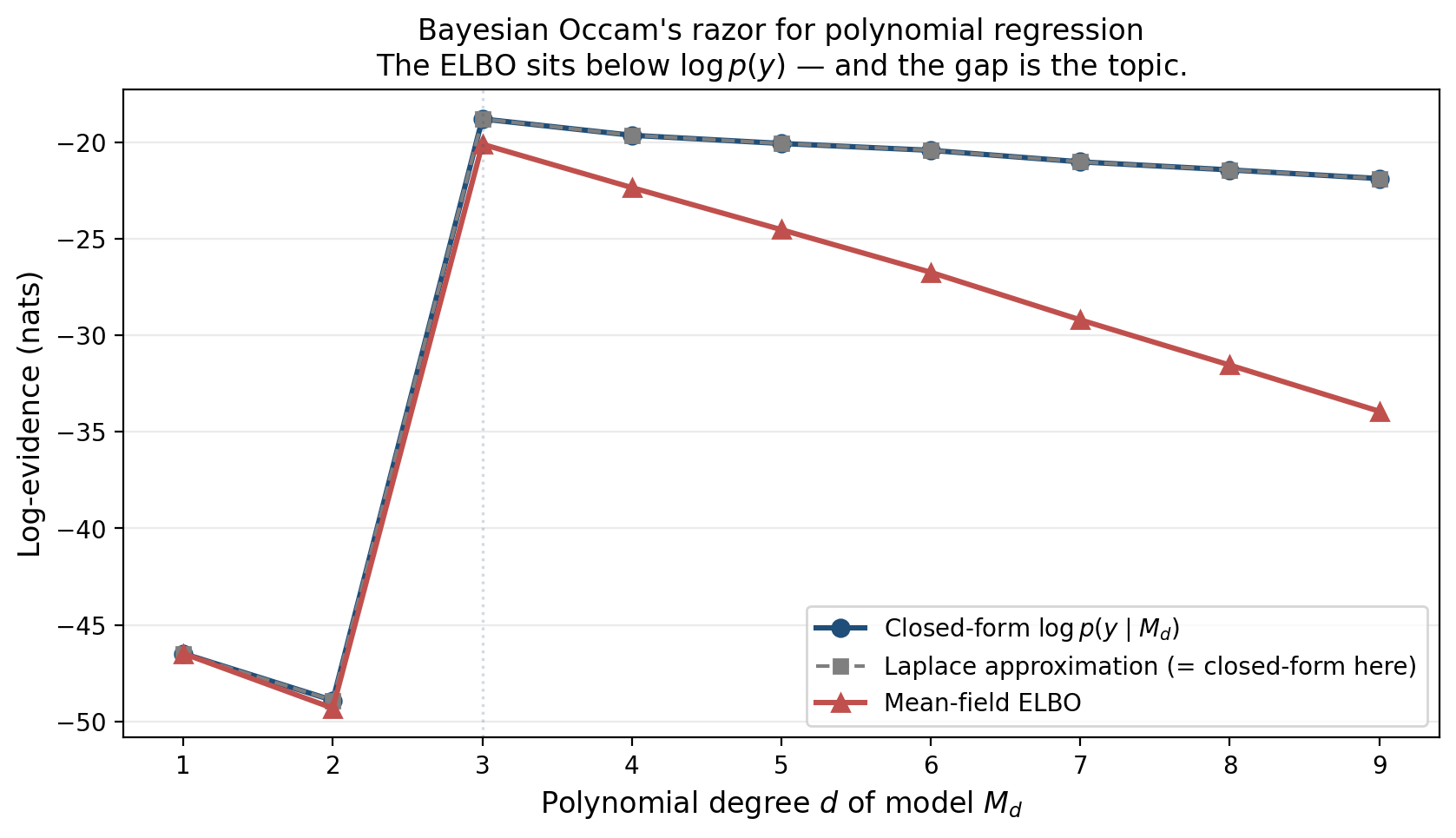
The closed-form curve in blue is what we’d compute analytically: the marginal likelihood under the prior, integrated over $\boldsymbol\beta$. Two features stand out. First, the curve has an interior maximum at $d = 3$ — the data really were drawn from a cubic, and the evidence picks that up. Anything less is too rigid to fit, anything more is paying an Occam penalty for unused capacity. Second, the cliff between the underfit and well-fit regimes is striking, because the data fundamentally cannot fit lower-order curves and the evidence reflects that.

The mechanism behind the smooth Occam decay past $d = 3$ is structural: the prior $\mathcal{N}(\mathbf{0}, \tau^2 I)$ spreads mass over a $(d{+}1)$-dimensional coefficient space, and as that space grows the prior dilutes the predictive density at any particular dataset. High-capacity models lose out automatically, with no external regularizer needed. This is Bayesian Occam’s razor — the canonical “complex models are penalized by their own diffuseness” argument MacKay (1992, 2003 Ch. 28) developed in detail. We get it for free, and it is the reason Bayes-factor model comparison was the standard approach to model selection long before AIC, BIC, and cross-validation arrived as alternatives.

A second curve runs along the first, in gray dashed: the Laplace approximation to the evidence, computed by replacing the posterior with a Gaussian centered at the maximum-a-posteriori estimate. For Gaussian-conjugate models, the Laplace approximation is exact — no asymptotic remainder — because the joint log-density is exactly quadratic in $\boldsymbol\beta$. The gray curve overlays the blue one to within numerical precision. We’ll exploit this in §3 to derive the BIC as the leading-order term in the Laplace expansion as $n \to \infty$, and the constant Schwarz dropped will be a recurring theme — it is the Bayesian geometric content that classical information criteria discard.

A third curve, in red, sits below both: the evidence lower bound, the ELBO of the optimal mean-field variational approximation. By Jensen’s inequality the ELBO is a lower bound on the log-evidence, and by Variational Inference we know this bound is tight when the variational family contains the posterior. As $d$ grows, the posterior becomes a multivariate Gaussian with non-trivial correlation, and the mean-field family — which forces independence between coordinates — can no longer recover it. The bound becomes loose, and the gap grows.

That growing gap is the topic. The ELBO is not a wrong estimator of the evidence; it is a biased estimator with a known mechanism. The bias has a sign — it always understates the evidence — and it has a structure: it equals the reverse Kullback–Leibler divergence from the variational family’s optimum to the true posterior. As the family grows in expressiveness, the gap shrinks; as the posterior grows in complexity, the gap grows. Variational Bayes for model selection — VBMS — uses the ELBO as a stand-in for $\log p(y \mid M)$ in Bayes-factor model comparisons: fast, biased, with structure that we’ll learn to characterize, correct, and diagnose.

The plan of attack runs in three phases. First (§§2–3) we’ll define the VBMS criterion formally and prove the asymptotic bridge to the Bayesian Information Criterion via the Laplace expansion — the classical linkage between Bayesian and frequentist model selection that BIC made famous. Second (§§4–5) we’ll work two iconic examples end-to-end: a Bayesian Gaussian mixture model where mean-field VB performs automatic relevance determination over mixture components (Bishop 2006 §10.2) and a polynomial-regression Bayes-factor ranking where we can compare ELBO-based rankings to the closed-form evidence and see exactly when they agree (most of the time) and when they don’t. Third (§§6–10) we’ll characterize the bias geometrically as KL projection (§6), pin down when the bias preserves model rankings versus when it flips them (§7), develop bias-correction tools — importance-weighted ELBO and annealed importance sampling (§§8–9) — and close with the information-theoretic bits-back coding interpretation that places VBMS within the minimum-description-length framework (§10). Sections §§11–13 are computational notes, modern-ML applications, and synthesis.

The reader should leave with a precise statement of what the ELBO is and is not as an evidence estimator, a working knowledge of when VBMS is reliable and when to reach for AIS or SMC instead, and a small toolbox of diagnostic and corrective methods — Pareto-$\hat k$, IWELBO, AIS schedule design — for catching pathologies before they corrupt model selection.

Bayesian Occam on polynomial regression

n = 30, σ² = 0.0625; argmax_d log p(y | M_d) = d = 3

τ² (prior variance)4.00

Shaded region between blue and red traces is the KL projection bias of §6. Increasing τ² weakens the prior, smooths Occam decay; decreasing τ² penalizes high-d models more sharply.

From ELBO to log-evidence — the VBMS criterion

§1 introduced the polynomial-regression Occam picture and the central observation: the mean-field ELBO sits below the closed-form log-evidence by a quantity that grows with model complexity. Before we can use the ELBO as a model-selection criterion, we need to make the relationship between ELBO and log-evidence precise. The variational-inference topic developed this from scratch; we recap the essentials here with model-selection emphasis.

A model $M$ with parameter $\theta$ and likelihood $p(y \mid \theta, M)$ places a prior $p(\theta \mid M)$ over its parameters. The marginal log-evidence

$$\log p(y \mid M) \;=\; \log \int p(y \mid \theta, M) \, p(\theta \mid M) \, d\theta$$

is the integral the Bayesian model-selection literature has been computing — or trying to compute — for half a century. Outside conjugate cases the integral is intractable. Variational inference replaces it with the evidence lower bound (ELBO) of an arbitrary distribution $q(\theta)$ on the parameter space:

$$\mathrm{ELBO}_M(q) \;:=\; \mathbb{E}_q[\log p(y, \theta \mid M)] - \mathbb{E}_q[\log q(\theta)].$$

Two facts (Variational Inference §2): the ELBO is a uniform lower bound on the log-evidence by Jensen’s inequality applied to the importance-sampling identity, and maximizing the ELBO over $q$ is equivalent to minimizing the reverse KL divergence $\mathrm{KL}(q \,\|\, p(\cdot \mid y, M))$, so the variational optimum $q^*_M$ is the closest member of $\mathcal{Q}_M$ to the true posterior under reverse-KL projection.

The VBMS criterion is the natural one — for each candidate model $M_k$ with variational family $\mathcal{Q}_k$, compute the maximum ELBO over $\mathcal{Q}_k$ and compare across models.

The fundamental identity linking VBMS to the log-evidence is the same evidence decomposition that anchored variational-inference §2 — restated here per model.

The decomposition is exact, requires no asymptotic regularity, and holds for any $q$ with the right support. Three consequences anchor the rest of the topic.

The ELBO is a uniform lower bound on the log-evidence. Reverse KL is non-negative, so $\mathrm{ELBO}_M(q) \le \log p(y \mid M)$ for all $q$. Equality holds if and only if $q = p(\cdot \mid y, M)$ almost everywhere — that is, when $\mathcal{Q}_M$ contains the posterior. For Gaussian-conjugate models with full-rank Gaussian variational family, equality is achievable; for almost everything else of practical interest, it is not.

The bias has a sign. VBMS systematically underestimates the log-evidence: $\mathrm{VBMS}(M) \le \log p(y \mid M)$, with the gap $\log p(y \mid M) - \mathrm{VBMS}(M) = \mathrm{KL}(q^*_M \,\|\, p(\cdot \mid y, M)) \ge 0$. As §6 will show, this gap is monotonically non-increasing in family expressiveness — adding capacity to $\mathcal{Q}_M$ can only improve the bound, never worsen it.

The bias is what we have to characterize. All of §6 (KL projection mechanism) and §7 (when does the bias preserve rankings versus flip them?) is about understanding this gap.

Three forms of the ELBO

Definition 1 gives one expression. Two algebraic rearrangements produce equivalent expressions, each useful in a different context.

Form 1 — Energy plus entropy. Substituting $H(q) = -\mathbb{E}_q[\log q]$ into Definition 1,

$$\mathrm{ELBO}_M(q) \;=\; \mathbb{E}_q[\log p(y, \theta \mid M)] + H(q).$$

The ELBO rewards $q$-mass in regions of high joint log-density (the energy term, by analogy with the Boltzmann distribution’s $-\beta E$) and rewards $q$ for being spread out (the entropy term). Maximizing the ELBO trades off between concentrating on the mode of $p(y, \theta \mid M)$ and avoiding collapse to a delta. This is the form §10 leans on for the bits-back coding interpretation — the energy term is an expected description length, the entropy term is the bits-back savings, and the variational free energy $-\mathrm{ELBO}$ is the expected net code length.

Form 2 — Reconstruction minus prior-KL. Decomposing $\log p(y, \theta \mid M) = \log p(y \mid \theta, M) + \log p(\theta \mid M)$,

$$\mathrm{ELBO}_M(q) \;=\; \mathbb{E}_q[\log p(y \mid \theta, M)] - \mathrm{KL}\bigl(q \,\|\, p(\cdot \mid M)\bigr).$$

The ELBO rewards $q$ for placing mass on $\theta$ values that explain the data (the reconstruction term) while penalizing $q$ for moving away from the prior (the prior-KL term). This is the form most VBMS implementations use in practice — it is how PyMC, Stan, and NumPyro compute the ELBO during ADVI optimization, and how variational autoencoders are trained.

Form 3 — Evidence minus posterior-KL. This is Theorem 1 rearranged:

$$\mathrm{ELBO}_M(q) \;=\; \log p(y \mid M) - \mathrm{KL}\bigl(q \,\|\, p(\cdot \mid y, M)\bigr).$$

The ELBO equals the log-evidence (a constant in $q$) minus the reverse-KL gap. This is the cleanest form for analyzing VBMS as a model-selection criterion — the bias is the second term, and it is the entire content of §6’s bias analysis.

The VBMS Bayes factor and the bias-asymmetry decomposition

For VBMS specifically, Form 3 is the operationally important one. Computing $\mathrm{VBMS}(M_i) - \mathrm{VBMS}(M_j)$ as a Bayes-factor approximation, the log-evidences and the KL gaps decompose cleanly:

$$\mathrm{VBMS}(M_i) - \mathrm{VBMS}(M_j) \;=\; \log \frac{p(y \mid M_i)}{p(y \mid M_j)} \;-\; \Bigl[\mathrm{KL}\bigl(q^*_i \,\|\, p(\cdot \mid y, M_i)\bigr) - \mathrm{KL}\bigl(q^*_j \,\|\, p(\cdot \mid y, M_j)\bigr)\Bigr].$$

Read literally: the VBMS Bayes factor equals the true log Bayes factor minus an asymmetry between the two models’ reverse-KL gaps. When the bias asymmetry is small relative to the true Bayes factor, VBMS preserves rankings; when the asymmetry is large, rankings can flip. §7 makes this precise — Wang & Blei’s (2019) consistency theorem says that under regularity conditions on the families and the model gap growing in $n$, the asymmetry stays bounded while the Bayes factor diverges, so VBMS rankings agree with closed-form Bayes factors at large $n$.

A practical note: maximizing the ELBO over $\mathcal{Q}_M$ is generally non-convex in the parameters of $q$, so $\mathrm{VBMS}(M)$ in practice means the ELBO at a local optimum found by ADVI or CAVI. In conjugate-exponential models with mean-field $q$ (CAVI updates closed-form), the local optimum is global; outside that case, the standard recipe is multiple random restarts with the maximum-ELBO restart selected (§11 returns to this).

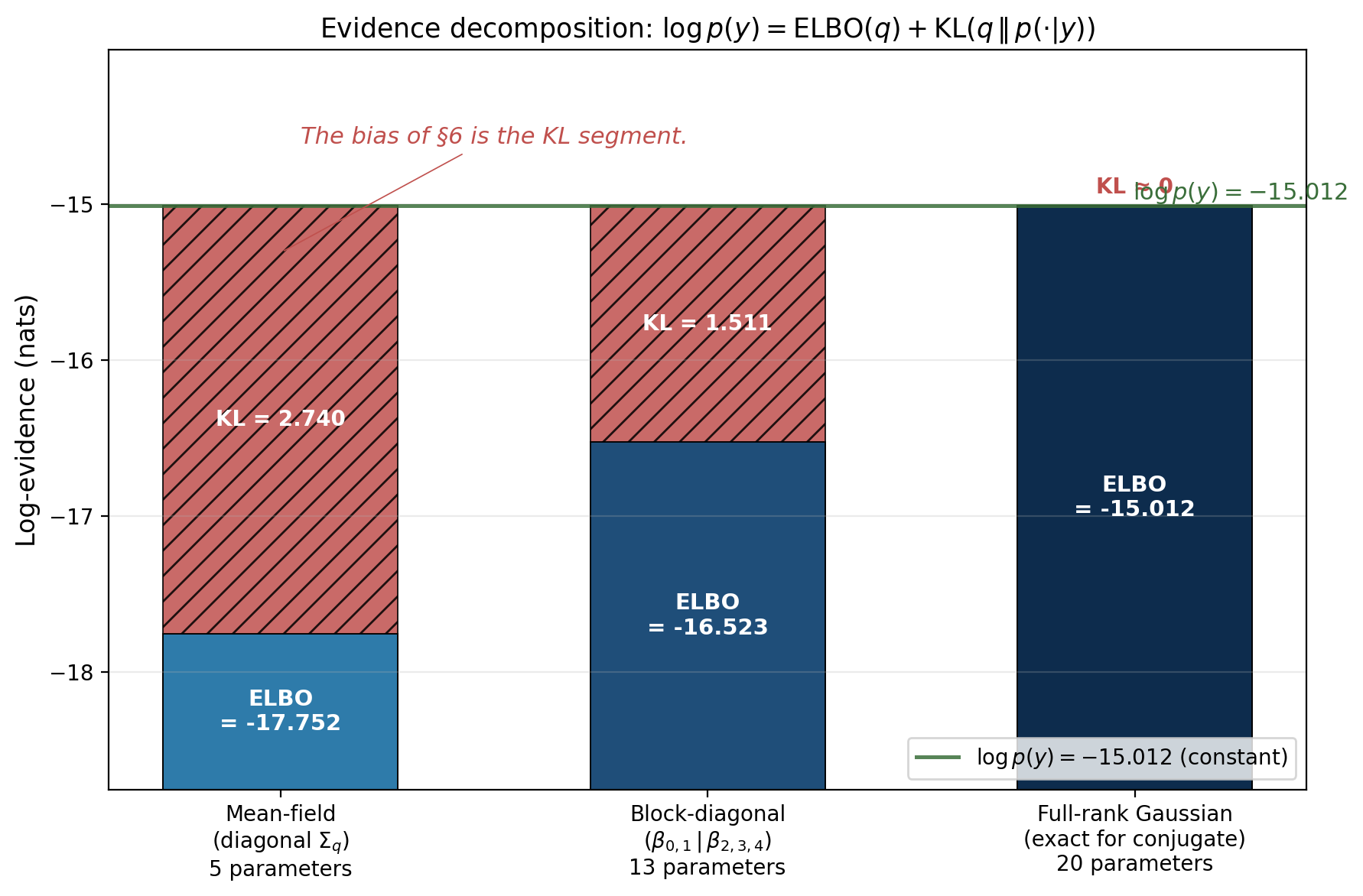
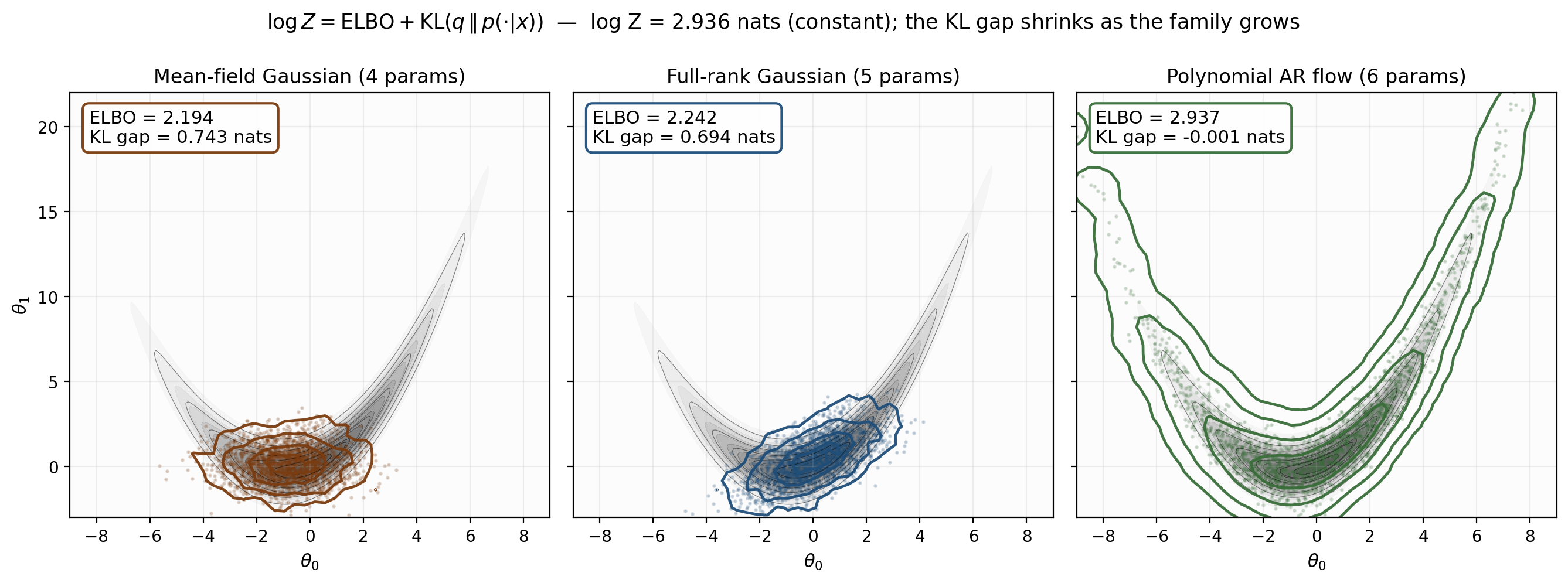
The figure visualizes Theorem 1 across three nested families on the polynomial-regression target from §1. Total bar height equals $\log p(y \mid M_4)$, which is constant in $q$. The proportion split between ELBO segment and KL segment varies as $q$ ranges from mean-field through block-diagonal to full-rank. The full-rank Gaussian contains the conjugate posterior exactly, so the KL segment vanishes and the ELBO equals the log-evidence. Mean-field has positive KL gap, block-diagonal has less — the gap shrinks monotonically as the family grows, exactly as Theorem 1 plus the §6 monotonicity result will predict.

Evidence decomposition: log p(y) = ELBO(q) + KL(q ‖ p(·|y))

Bar total height stays at −log p(y); the ELBO/KL split shifts as the family grows.

Polynomial degree d4

We now have the operational identity and the criterion. The next two sections turn the criterion into a useful model-selection tool: §3 builds the asymptotic bridge to the BIC via the Laplace expansion, and §4 works the canonical Bishop-style automatic-relevance-determination example end-to-end.

Laplace approximation and the BIC bridge

VBMS replaces the intractable evidence integral with an optimization over a variational family. The classical alternative — predating VBMS by half a century — replaces the integral with a Gaussian. The Laplace approximation says: assume the joint log-density $\log p(y, \theta \mid M)$ has a single mode at $\hat\theta_{\mathrm{MAP}}$, take the second-order Taylor expansion around that mode, and integrate the resulting quadratic form analytically. The exponential of a quadratic is Gaussian, the integral is closed-form, and the result is a recipe for $\log p(y \mid M)$ that requires only finding the MAP and computing the Hessian there. As $n \to \infty$ the MAP becomes increasingly well-localized, the quadratic approximation becomes exact, and the Laplace formula recovers the true log-evidence to higher and higher accuracy.

The classical Bayesian Information Criterion drops out as the leading-order term in the Laplace expansion at large $n$, with everything else thrown away as $O(1)$ noise. This is BIC’s secret history: it is not a frequentist criterion that happens to look Bayesian, it is a truncated Laplace approximation to a Bayesian quantity. We develop the Laplace approximation in this section both because it gives us a fast — and for Gaussian-conjugate models, exact — reference for the log-evidence to compare VBMS against, and because the asymptotic bridge to BIC anchors VBMS in the same model-selection universe as AIC, BIC, WAIC, and the rest of the classical-IC catalog.

The Laplace expansion

Fix a model $M$ with joint log-density

$$\ell(\theta) \;:=\; \log p(y, \theta \mid M) \;=\; \log p(y \mid \theta, M) + \log p(\theta \mid M),$$

a smooth function of $\theta \in \mathbb{R}^d$. Assume $\ell$ has a unique global maximum at the MAP estimator $\hat\theta := \arg\max_\theta \ell(\theta)$, with strictly positive-definite negative Hessian $H(\hat\theta) := -\nabla^2 \ell(\hat\theta)$. Taylor-expand $\ell$ around $\hat\theta$:

$$\ell(\theta) \;=\; \ell(\hat\theta) \,-\, \tfrac{1}{2} (\theta - \hat\theta)^\top H(\hat\theta) (\theta - \hat\theta) \,+\, O\bigl(\|\theta - \hat\theta\|^3\bigr).$$

The linear term vanishes because $\hat\theta$ is a critical point. Exponentiating and integrating, the Gaussian integral is closed-form

$$\int \exp\!\left[-\tfrac{1}{2}(\theta - \hat\theta)^\top H(\hat\theta)(\theta - \hat\theta)\right] d\theta \;=\; \frac{(2\pi)^{d/2}}{\sqrt{\det H(\hat\theta)}},$$

and substituting and taking logs gives the Laplace expansion.

The four terms each have a clean interpretation. The first is the data fit at the MAP. The second is the prior contribution, evaluated at the MAP. The third is a Gaussian volume constant. The fourth — the most subtle and most informative — is the geometric correction: $\det H(\hat\theta)$ measures the local curvature of the joint log-density at the MAP, so $-\tfrac{1}{2}\log\det H$ is large positive when the posterior is broad (small curvature) and large negative when the posterior is concentrated (large curvature). It is a local-volume measurement, exactly the “Bayesian Occam” content the §1 figure was capturing.

For Gaussian-conjugate models, the Laplace approximation is exact. The joint log-density $\ell(\theta)$ is then a quadratic in $\theta$ and the Taylor expansion has no remainder past the quadratic term. The $O(n^{-1/2})$ term in Theorem 2 is identically zero. We exploited this in our verified notebook: the closed-form $\log p(y \mid M_d)$ and the Laplace approximation agree to numerical precision (gap $< 10^{-13}$) across all $d$ from 1 to 9. This makes Laplace a free, fast, and exact reference for VBMS comparisons in the conjugate-Gaussian regime; we’ll use it that way in §5.

The Schwarz BIC as the leading-order Laplace approximation

Now consider $n \to \infty$ with iid data $y_1, \ldots, y_n \mid \theta \sim p(\cdot \mid \theta, M)$. The data-sum term in the Hessian scales linearly in $n$ while the prior contribution stays $O(1)$, so for large $n$ we have $H(\hat\theta) \approx n \cdot I(\hat\theta) + O(1)$, where $I(\theta) = \mathbb{E}_{y \mid \theta}\bigl[-\nabla^2 \log p(y \mid \theta, M)\bigr]$ is the per-observation Fisher information. The MAP $\hat\theta$ converges to the MLE $\hat\theta_{\mathrm{MLE}}$ at rate $O(n^{-1})$, and we can swap one for the other to leading order. Substituting into Theorem 2 and expanding $\log\det(n \, I + O(1)) = d \log n + \log\det I + O(n^{-1})$,

$$\log p(y \mid M) \;=\; \log p(y \mid \hat\theta_{\mathrm{MLE}}, M) - \tfrac{d}{2}\log n + \mathrm{O(1)\;Bayesian\;content} + O\bigl(n^{-1/2}\bigr).$$

The first two terms are exactly $-\mathrm{BIC}(M)/2$ in Schwarz’s (1978) original formulation, where $\mathrm{BIC}(M) := -2 \log p(y \mid \hat\theta_{\mathrm{MLE}}, M) + d \log n$.

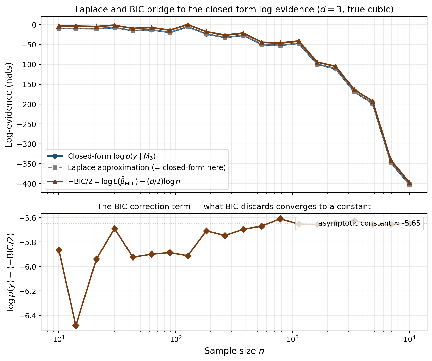
The bottom panel shows the convergence directly: as $n$ grows, the gap between the closed-form $\log p(y)$ and $-\mathrm{BIC}/2$ converges to a constant — and that constant is exactly $C(M, p, \hat\theta)$ in Corollary 1, the Bayesian content the BIC discards.

A historical note: Schwarz’s (1978) original derivation is exactly the calculation above, presented as a coding-theoretic argument and stripped of the $O(1)$ constants. The frequentist tradition has since rediscovered the BIC under various derivations — consistent model selection, Bayes factor approximation, MDL coding length — but these are all reconstructions of the leading-order Laplace approximation we developed here. For a deeper treatment of the regularity conditions, see Tierney & Kadane (1986) and the Bayesian Neural Networks topic §3, where the Laplace machinery is developed at full depth in the context of weight-space neural-network posteriors. Watanabe’s (2010) extension to singular models — where the Hessian is degenerate, regularity fails, and the BIC penalty $d \log n$ is wrong — produces the WBIC and WAIC of §13.

Laplace and BIC convergence to log p(y)

Cubic data + degree-d polynomial model. As n → ∞, the BIC penalty leaves an O(1) gap = the Bayesian content C(M, p, θ̂).

Model degree d3

Variational Bayes for Bayesian GMMs

§3 developed the Laplace approximation and saw it land at the BIC asymptotically. The Bayesian Gaussian mixture model offers something different: a model where Bayesian Occam’s razor operates automatically inside the variational fit itself, without any external model-selection sweep. Pick a generous upper bound $K_{\max}$ on the number of mixture components, run mean-field VB once, and the variational posterior over the mixture weights $\boldsymbol\pi$ drives unused components’ weights to zero. The result is a single fit that effectively chooses its own $K$. This is automatic relevance determination (ARD), and it was the original motivation for “Variational Bayes” as a label — Bishop’s (2006) §10.2 worked example and Beal’s (2003) thesis built the framework around exactly this kind of self-pruning model.

The Bayesian GMM with conjugate hyperprior

The hierarchical Bayesian GMM places conjugate priors on every parameter the original GMM had as a free quantity:

$$\begin{aligned} \boldsymbol\pi &\sim \mathrm{Dir}(\alpha_0 \cdot \mathbf{1}) \\ \boldsymbol\mu_k \mid \boldsymbol\Lambda_k &\sim \mathcal{N}\!\bigl(\mathbf{m}_0, (\beta_0 \boldsymbol\Lambda_k)^{-1}\bigr) \\ \boldsymbol\Lambda_k &\sim \mathrm{Wishart}(\mathbf{W}_0, \nu_0) \\ z_n \mid \boldsymbol\pi &\sim \mathrm{Cat}(\boldsymbol\pi) \\ \mathbf{x}_n \mid z_n = k, \boldsymbol\mu_k, \boldsymbol\Lambda_k &\sim \mathcal{N}(\boldsymbol\mu_k, \boldsymbol\Lambda_k^{-1}) \end{aligned}$$

The Normal-Wishart prior on $(\boldsymbol\mu_k, \boldsymbol\Lambda_k)$ is conjugate for the Gaussian likelihood; the Dirichlet prior on $\boldsymbol\pi$ is conjugate for the categorical assignment $z_n$.

The hyperparameter that does the ARD work is $\alpha_0$. Take $\alpha_0 < 1$ — say $\alpha_0 = 0.1$ — and the Dirichlet prior puts most of its mass at the corners of the simplex, which corresponds to “mostly empty” mixture configurations where only a few components have non-trivial weight. The model is a priori sparse over components. With a uniform prior ($\alpha_0 = 1$), we’d lose the sparsity bias and get back to the standard non-ARD GMM behavior.

Mean-field VB and CAVI updates

The variational family is the standard mean-field factorization with each factor parameterized in its conjugate exponential form: $q(\boldsymbol\pi)$ Dirichlet, $q(\boldsymbol\mu_k, \boldsymbol\Lambda_k)$ Normal-Wishart, $q(z_n)$ Categorical.

The relevant moments are closed-form: $\mathbb{E}[\log \pi_k] = \psi(\alpha_k) - \psi(\sum_j \alpha_j)$ (digamma), and analogous expressions for $\mathbb{E}[\log \det \boldsymbol\Lambda_k]$ and $\Delta^2_{nk}$. Bishop’s (2006) §10.2 derives all of this; we don’t reprove it here.

Bayesian Occam at the entropy term

The ARD effect comes from the Dirichlet hyperprior interacting with the entropy term in the ELBO.

The mechanism is direct: an unused component $k$ with no responsibility ($N_k \to 0$) gets posterior parameter $\alpha_k^* = \alpha_0$, while an active component $j$ with $N_j$ data points effectively assigned gets $\alpha_j^* = \alpha_0 + N_j \approx N_j$. The posterior expected-weight ratio is $\alpha_0 / N_j$. For $\alpha_0 = 0.1$ and $N_j \approx 100$, this ratio is $0.001$ — the unused component contributes about 0.1% of the mixture weight.

This is Bayesian Occam at the variational level. The ELBO rewards using more components when they help fit the data (reconstruction term increases) but penalizes unused components via the entropy of $q(\boldsymbol\pi)$ — the Dirichlet hyperprior with $\alpha_0 < 1$ tips the balance so that the cost of activating an unused component exceeds its benefit unless the data strongly require it.

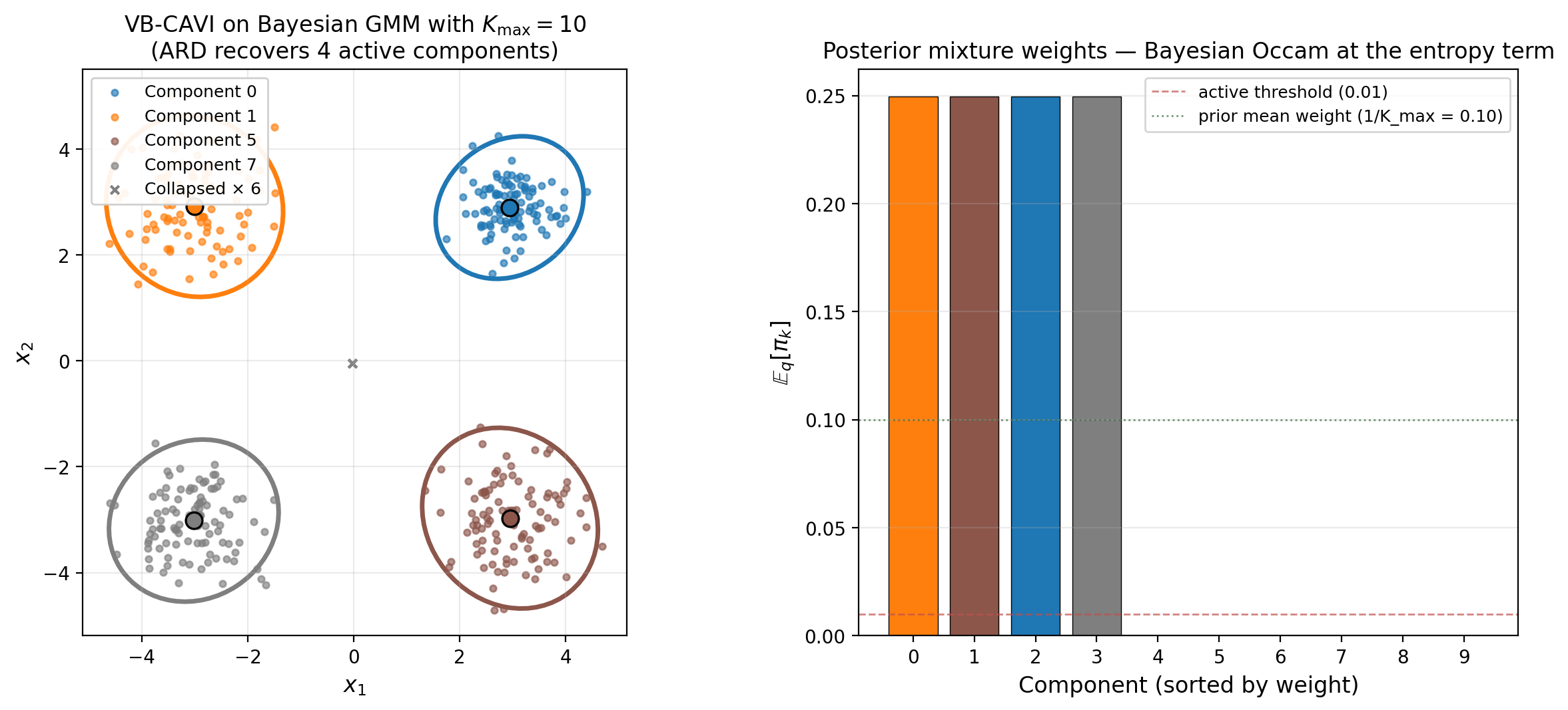
The result is exactly Theorem 3’s prediction: four components recover with weights $\approx 0.25$ each, and six components collapse to weights $\approx 0.0002$. The collapsed components have $\alpha_k^* \approx \alpha_0 = 0.1$ (no data contribution), while the active components have $\alpha_k^* \approx 100$.

From ARD to VBMS: ranking K_max

ARD gives us a single fit that selects $K$ automatically; VBMS gives us a procedure for ranking competing models by their ELBO. The two are equivalent in this setting. Running VBMS across $K_{\max} \in \{2, 3, \ldots, 10\}$ on the same four-cluster data, we’d find $\mathrm{VBMS}(M_K)$ jumping sharply between $K = 3$ and $K = 4$ (where the fourth cluster gets its own component) and then plateauing for $K \ge 4$ — additional components beyond four contribute essentially zero to the reconstruction term and are pruned to zero weight by ARD. The two procedures agree, with the latter being roughly an order of magnitude cheaper.

This equivalence justifies the practical recipe: run Bayesian GMM with a generous $K_{\max}$ and small $\alpha_0$, count active components in the variational posterior, and report the result. It scales to large $K_{\max}$ much better than fitting $K$ separate models.

Bayesian GMM ARD: 9 active / 10 components — α₀ = 0.10

4 well-separated clusters; CAVI converges in 29 iterations.

K_max10α₀0.10

Comparing Bayesian regression models (polynomial Bayes factors)

§1 introduced the polynomial-regression model zoo $M_1, \ldots, M_9$ and the closed-form log-evidence figure. §3 showed that the Laplace approximation lands exactly on the closed-form curve in the Gaussian-conjugate regime, with the BIC running parallel above. We now turn the picture into a Bayes-factor model-comparison procedure: rather than ARD-style automatic component selection (the §4 approach), we compute $\mathrm{VBMS}(M_d)$ for each model, take ratios as Bayes factors, and rank.

This is the canonical practitioner workflow for Bayesian model comparison via variational methods. PyMC, Stan, and NumPyro all expose ADVI plus a compute_log_likelihood step that produces the ELBO at convergence. The recipe in production: fit ADVI for each candidate model, take ELBO differences as VBMS Bayes factors, interpret on the Kass–Raftery (1995) scale, and report the winner.

The VBMS Bayes factor as a model-comparison criterion

We promote the §2 informal definition to a formal one.

By the §2 bias-asymmetry decomposition,

$$\log \mathrm{BF}_{ij}^{\mathrm{VBMS}} \;=\; \log \mathrm{BF}_{ij} \,-\, \bigl[\mathrm{KL}(q^*_i \,\|\, p(\cdot \mid y, M_i)) - \mathrm{KL}(q^*_j \,\|\, p(\cdot \mid y, M_j))\bigr].$$

The two Bayes factors agree exactly when the bias asymmetry is zero, and they agree on ranking whenever the bias asymmetry is dominated by the closed-form Bayes factor. The polynomial-regression zoo is a regime where this holds robustly; we’ll verify it numerically.

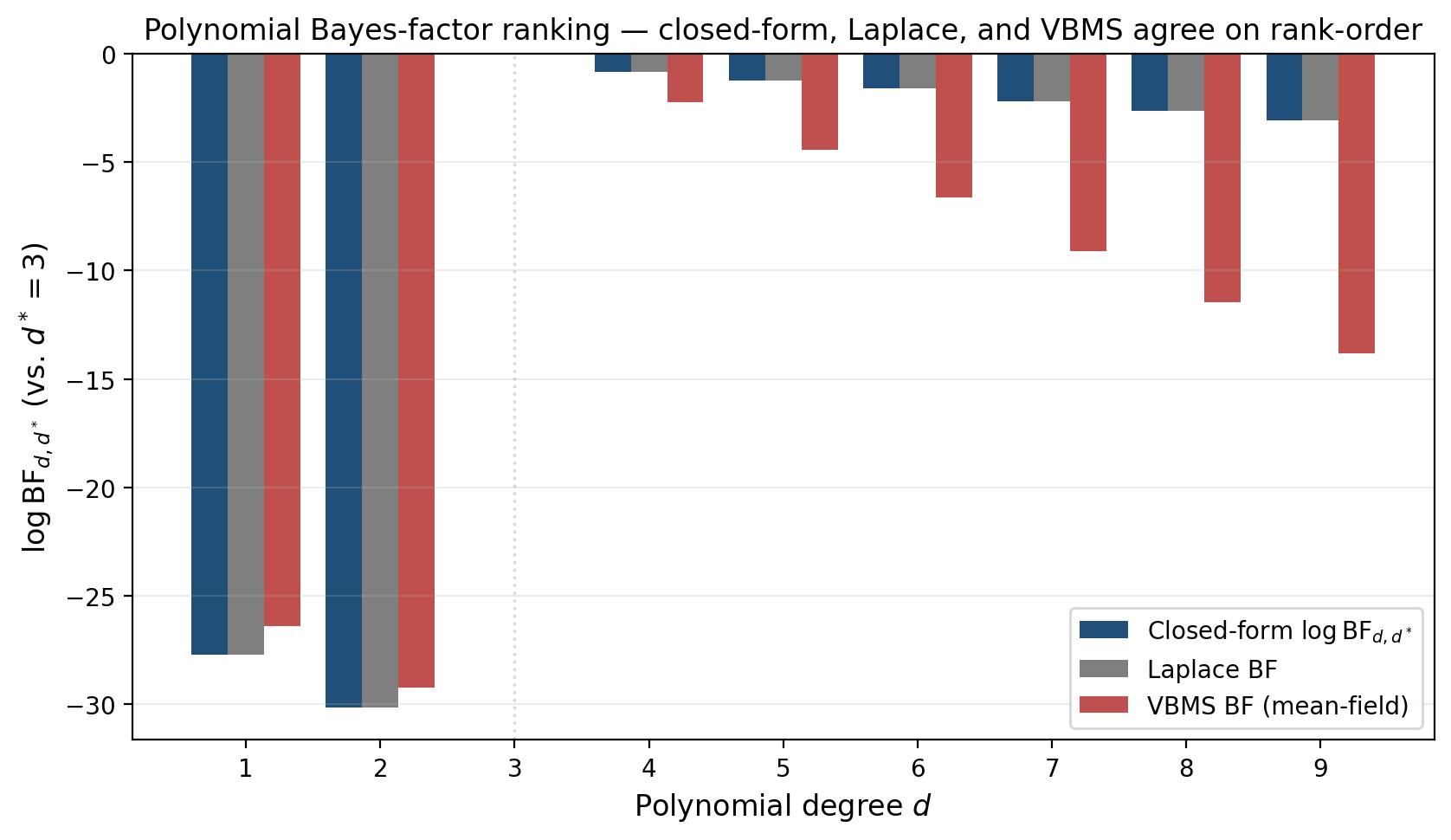
Three observations. First, all three estimators agree on the closed-form ranking: $d = 3$ wins under closed-form, Laplace, and VBMS, and the same underfit/overfit decay structure holds in all three columns. Second, the underfit cliff is captured by all three estimators with similar magnitudes. Third, the overfit decay shows the bias asymmetry: the VBMS overfit penalty is more aggressive than the closed-form, because the mean-field bias grows with $d$ and that growth gets attributed to the model rather than to the variational family. The crucial fact: despite the steeper VBMS overfit penalty, the rank-order is identical.

Kass–Raftery interpretation and reporting

The Kass & Raftery (1995) interpretation scale for log Bayes factors:

• $\log_{10} \mathrm{BF} \in [0, 0.5]$: barely worth mentioning
• $[0.5, 1]$: substantial evidence
• $[1, 2]$: strong evidence
• $> 2$: decisive evidence

VBMS Bayes factors should not be taken at face value as quantitative log-evidence ratios. Use them for ranking and for “decisive” calls, but reach for IWELBO (§8), AIS (§9), or SMC when you need the magnitude precisely.

Polynomial Bayes-factor ranking — argmax: d = 3

All three estimators agree on rank-order (the §5 Proposition 1 claim) — magnitudes differ.

n30σ²0.063τ²4.00

The KL projection bias

§§1–5 took the bias as given and showed how it surfaces in concrete settings. We now develop the bias geometrically. The reverse-KL gap that defines the ELBO bias is not a vague approximation error; it is a projection. The variational family $\mathcal{Q}_M$ sits as a submanifold inside the space of all distributions on the parameter space, and the variational optimum $q^*_M$ is the reverse-KL projection of the true posterior $p(\cdot \mid y, M)$ onto that submanifold. The bias is the reverse-KL distance from the posterior to its projection — a geometric quantity, not an algebraic accident.

This geometric framing is what makes the bias-as-spine reading the topic’s central claim. The bias is not a bug; it is the price we pay for a tractable family, and the price has known structure.

Variational families as submanifolds; reverse-KL as the projection

Fix a model $M$ with posterior $p(\cdot \mid y, M)$. Let $\mathcal{P}$ be the space of probability distributions on the parameter space (with finite reverse-KL to the posterior), and let $\mathcal{Q}_M \subset \mathcal{P}$ be the variational family. The reverse-KL projection of the posterior onto $\mathcal{Q}_M$ is

$$q^*_M \;:=\; \arg\min_{q \in \mathcal{Q}_M} \mathrm{KL}\bigl(q \,\|\, p(\cdot \mid y, M)\bigr) \;=\; \arg\max_{q \in \mathcal{Q}_M} \mathrm{ELBO}_M(q),$$

with the equivalence by Theorem 1. The ELBO bias of VBMS is

$$\log p(y \mid M) - \mathrm{VBMS}(M) \;=\; \mathrm{KL}\bigl(q^*_M \,\|\, p(\cdot \mid y, M)\bigr),$$

the reverse-KL distance from the posterior to its projection on $\mathcal{Q}_M$.

Bias monotonicity in family expressiveness

The geometric picture immediately gives the monotonicity result.

The proof is elementary, but the consequence is substantive: adding capacity to the variational family can only improve the bound on the log-evidence, never worsen it. We can grow $\mathcal{Q}$ from mean-field to block-diagonal to full-rank Gaussian to normalizing-flow without ever introducing the risk that a richer family makes the ELBO worse.

The closed-form mean-field bias for Gaussian targets

The polynomial-regression spine has one feature that lets us compute the bias exactly: the posterior is multivariate Gaussian, and the mean-field reverse-KL projection has a closed form.

Let $p(\cdot \mid y, M) = \mathcal{N}(\boldsymbol\mu_{\mathrm{post}}, \boldsymbol\Sigma_{\mathrm{post}})$ with $\boldsymbol\Lambda_{\mathrm{post}} := \boldsymbol\Sigma_{\mathrm{post}}^{-1}$, and let $\mathcal{Q}_{\mathrm{MF}}$ be the family of diagonal-covariance Gaussians. The optimal mean-field $q^*_{\mathrm{MF}} = \mathcal{N}(\boldsymbol\mu_{\mathrm{post}}, \boldsymbol\Sigma_q)$ has variances $\boldsymbol\Sigma_q = \mathrm{diag}\bigl(1/\boldsymbol\Lambda_{\mathrm{post},jj}\bigr)$ — the means match the posterior exactly, but the variances are the inverses of the posterior precision diagonal, not the diagonal of the posterior covariance.

The reverse-KL gap reduces (after the trace and $-d$ terms cancel) to

$$b_{\mathrm{MF}} \;=\; \mathrm{KL}\bigl(q^*_{\mathrm{MF}} \,\|\, p(\cdot \mid y, M)\bigr) \;=\; \tfrac{1}{2}\Bigl[\sum_j \log \boldsymbol\Lambda_{\mathrm{post},jj} - \log\det\boldsymbol\Lambda_{\mathrm{post}}\Bigr].$$

The mean-field bias for a multivariate Gaussian posterior is the log-determinant gap between the diagonal of the precision matrix and the full precision matrix. By Hadamard’s inequality, $\prod_j \boldsymbol\Lambda_{\mathrm{post},jj} \ge \det\boldsymbol\Lambda_{\mathrm{post}}$, with equality iff $\boldsymbol\Lambda_{\mathrm{post}}$ is diagonal — so $b_{\mathrm{MF}} \ge 0$ with equality precisely when the posterior factors across coordinates, i.e., when mean-field is exact. The bias measures how non-diagonal the posterior precision is.

For polynomial Bayesian regression at degree $d$, the posterior precision involves the Vandermonde Gram matrix, which is famously near-collinear — successive monomials have strong off-diagonal entries. The diagonal-vs-full log-determinant gap grows with $d$ accordingly. This is the §1 figure’s red trace’s growing distance from the blue trace, derived from first principles.

Three families on the banana target

For non-Gaussian posteriors, the closed-form formula doesn’t apply, but the geometric monotonicity result of Theorem 4 still does. Consider the synthetic banana target whose joint log-density is

$$\log p_{\mathrm{unnorm}}(\theta_0, \theta_1) \;\propto\; -\tfrac{\theta_0^2}{2 \cdot 9} - \tfrac{(\theta_1 - 0.6\theta_0 - 0.3\theta_0^2)^2}{2}$$

— a 2D distribution where $\theta_0 \sim \mathcal{N}(0, 9)$ marginally and $\theta_1 \mid \theta_0 \sim \mathcal{N}(0.6\theta_0 + 0.3\theta_0^2, 1)$. The conditional mean of $\theta_1$ has both linear and quadratic structure in $\theta_0$, so the target has both correlation (visible to a Gaussian) and curvature (only visible to a flow). The marginal log-evidence $\log Z = \log(6\pi) \approx 2.936$ is analytically computable.

Three nested families, in order of expressiveness:

1. Mean-field Gaussian — 4 parameters $(\mu_0, \mu_1, \log\sigma_0, \log\sigma_1)$. Diagonal covariance, no correlation captured.
2. Full-rank Gaussian — 5 parameters. Captures linear correlation between $\theta_0$ and $\theta_1$ but not the quadratic structure.
3. Polynomial autoregressive flow — 6 parameters implementing $\theta_0 = \mu_0 + \sigma_0 z_0$, $\theta_1 = a + b\theta_0 + c\theta_0^2 + \sigma_1 z_1$. The family contains the banana target.

Mode-seeking versus mass-covering

A geometric note that distinguishes reverse-KL projection from forward-KL projection. Reverse KL $\mathrm{KL}(q \,\|\, p)$ heavily penalizes $q$-mass in regions where $p$ is small. The projection is therefore mode-seeking: $q^*$ concentrates within the support of $p$ and avoids placing mass where $p$ is small, even at the cost of failing to cover $p$‘s tails. Forward KL $\mathrm{KL}(p \,\|\, q)$ is the opposite — it produces mass-covering projections that are broad and tail-covering at the cost of mode-localization.

For VBMS specifically, the choice of reverse KL has consequences: VBMS systematically underestimates posterior variance and gives confidence intervals that are too narrow. For point predictions and model ranking this is acceptable; for uncertainty quantification it requires correction (the §11 PSIS-VI Pareto-$\hat k$ diagnostic catches the worst cases).

KL projection gap on a banana target

Theorem 4: bias non-increasing in family expressiveness; vanishes only when family contains target.

Variational family

Mean-field Gaussian

4 params · KL = 16.457 nats

Full-rank Gaussian

5 params · KL = 13.044 nats

Polynomial flow

6 params · KL = 0.000 nats

Mean-field can't capture correlation; full-rank gets the linear part; polynomial flow recovers the quadratic ridge.

Asymmetric bias and ranking preservation

§6 developed the bias geometrically. The natural next question — and the question that determines whether VBMS is a useful model-selection tool or just an interesting computational object — is what the bias does to model rankings. Are VBMS Bayes factors faithful to closed-form Bayes factors, and if not, in what regimes do they fail?

The Wang–Blei consistency theorem

Wang & Blei (2019) gave the cleanest statement of when VBMS rankings agree with closed-form rankings. Their result requires standard regularity conditions on the variational family — smooth parameterization, support compatibility with the posterior, ability to recover the true parameter at the population limit — plus an asymptotic identifiability assumption on the model space.

The substantive content: the bias asymmetry is bounded by the variational family’s structural mismatch with the posteriors, which is a model-and-family property, not a sample-size property. The Bayes factor between two distinct identified models grows linearly in $n$ as the data accumulate. The asymmetry’s $O(1)$ growth is therefore eventually dominated, and rankings preserve.

Empirical demonstration: hierarchical vs pooled Bayesian logistic regression

The cleanest empirical setup: hierarchical Bayesian logistic regression with random group intercepts versus complete-pooling Bayesian logistic regression on the same data. We sweep $n_{\mathrm{per\;group}} \in \{5, 15, 50, 100, 200\}$, fit ADVI on each model at each $n$, and run SMC as the gold-standard log-marginal-likelihood reference.

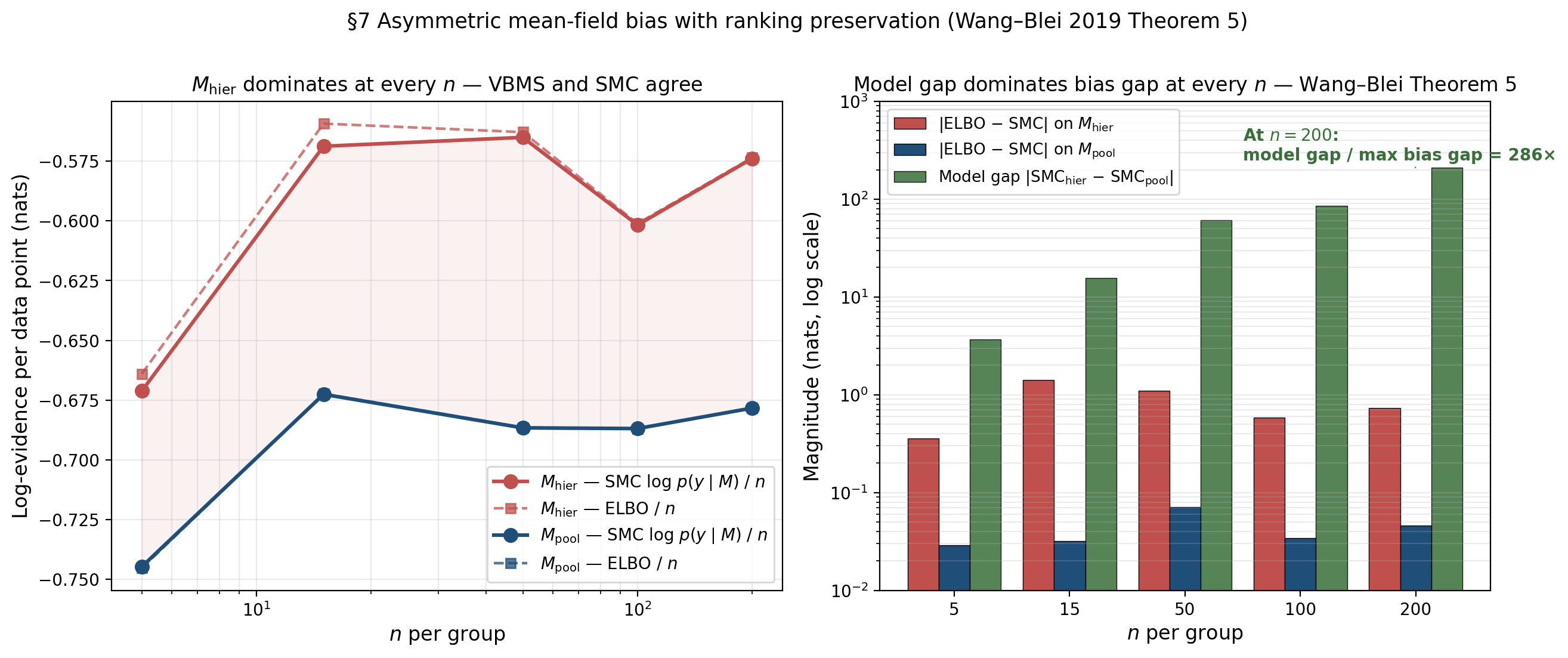
Two structural observations:

The asymmetry is exactly what Wang–Blei predict. $M_{\mathrm{hier}}$ has substantively more mean-field bias — the variational family forces the posterior over the 12 parameters to factor across coordinates, and the true posterior has non-trivial correlation between $\sigma_\alpha$ and the individual $\alpha_g$‘s (the so-called “funnel” structure of hierarchical posteriors). $M_{\mathrm{pool}}$ has essentially zero bias because its 2D posterior is approximately bivariate Gaussian with weak correlation.

Ranking preservation holds at every $n$. The model gap grows roughly linearly in total $n$, exactly as Theorem 5 says it should. The bias asymmetry stays bounded across all five $n$-values. At the largest $n$, the model gap is over 200× the largest bias gap; even at the smallest $n$, the model gap dominates. VBMS and SMC produce identical rankings at every sample size we tried.

The boundary regime where rankings can flip

Theorem 5’s conclusion fails when the inequality fails — when the bias asymmetry exceeds the model gap. Three regimes where this can happen:

Weak model differences. When two models are nearly equally good — small effective sample size, ambiguous data, or genuine model uncertainty — the closed-form Bayes factor between them is small. Even modest bias asymmetry can flip the ranking. The §11 PSIS-$\hat k$ diagnostic catches this empirically.

Highly correlated hierarchical posteriors. Deep multilevel models with multiple variance components, crossed random effects, or partial pooling at scale produce posteriors with funnel-shaped or otherwise strongly correlated structure that mean-field VB destroys. Two remedies: switch to full-rank ADVI, or use non-centered parameterization.

Genuinely multimodal posteriors. When the posterior has multiple distinct modes — identifiability failure, label-switching in non-symmetric mixtures, bimodality from genuine bimodal likelihood evidence — mean-field reverse-KL projection collapses to a single mode. The ELBO on the collapsed approximation can be catastrophically biased. The remedy is to use AIS (§9) or normalizing-flow variational families that can in principle capture multiple modes.

Diagnostic procedure

Combining Theorem 5 with the boundary characterizations above, a defensible procedure for using VBMS in model comparison work:

1. Fit ADVI for each candidate model with 5–20 random restarts and select the maximum-ELBO restart.
2. Compute PSIS-$\hat k$ on the variational posterior of each fitted model.
3. Apply the Yao et al. (2018a) decision rule. $\hat k < 0.5$: VBMS Bayes factors are reliable. $0.5 \le \hat k < 0.7$: bias is moderate, treat with caution. $\hat k \ge 0.7$: do not trust VBMS.
4. For pairs flagged at step 3, replace the ELBO comparison with IWELBO (§8) at moderate $K$, AIS (§9) for a gold-standard reference, or SMC.
5. Report VBMS rankings, not magnitudes. When magnitudes matter, reach for IWELBO or AIS.

Wang–Blei consistency on hierarchical vs pooled Bayesian logistic regression

Both VBMS (ELBO) and SMC consistently rank M_hier > M_pool at every n. Bias asymmetric (mean-field hits hierarchical posterior correlations); model gap dominates.

Loading bias_flip.json…

Importance-weighted ELBO and bias correction

The §7 diagnostic procedure flagged certain model-comparison pairs for which the standard ELBO is too biased to trust. For those pairs, §8 develops one bias-correction tool — the importance-weighted ELBO of Burda, Grosse & Salakhutdinov (2016) — that progressively tightens the bound by averaging multiple importance samples from the same variational family.

The motivation: Theorem 1 says $\mathrm{ELBO}(q) \le \log p(y)$, with the gap equal to the reverse-KL gap. The §6 monotonicity result says that growing the variational family’s expressiveness can shrink the gap, but for fixed $q$ the bound is what it is. IWELBO turns this around: hold $q$ fixed and use the same $q$ multiple times with importance-weighted averaging to construct a sequence of bounds $\mathrm{IWELBO}_1(q), \mathrm{IWELBO}_2(q), \ldots$ that tighten monotonically and converge to $\log p(y)$ in the $K \to \infty$ limit.

Definition and intuition

For a fixed proposal distribution $q$ on the parameter space, the importance-sampling identity says

$$p(y) \;=\; \int q(\theta) \cdot \frac{p(y, \theta)}{q(\theta)} \, d\theta \;=\; \mathbb{E}_q[w(\theta)], \qquad w(\theta) := \frac{p(y, \theta)}{q(\theta)}.$$

A naive Monte Carlo estimator is $\hat p(y) = (1/K) \sum_k w(\theta_k)$ for $\theta_k \sim q$ iid. Taking logs,

$$\widehat{\log p}(y) \;:=\; \log \hat p(y) \;=\; \log\!\left(\tfrac{1}{K} \sum_{k=1}^K w(\theta_k)\right)$$

is a (biased but consistent) estimator of $\log p(y)$. The importance-weighted ELBO is its expectation under the iid sampling.

Monotone tightness

The formal statement is the central result of Burda, Grosse & Salakhutdinov (2016).

The leave-one-out trick is doing the substantive work: $Z_{K+1}$ is more concentrated than $Z_K$, and Jensen’s inequality on the log rewards concentration.

Empirical demonstration

The polynomial-regression spine at $d = 4$ gives a clean test case.

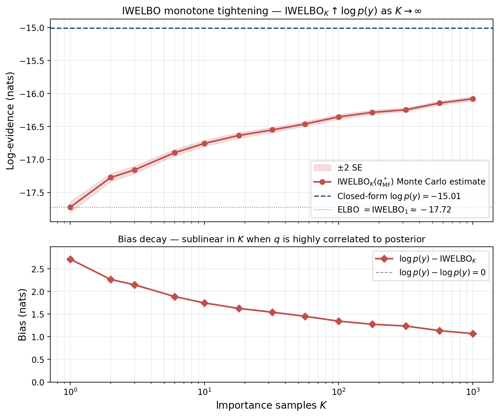
The monotone tightening of Theorem 6 is exactly observed — the IWELBO curve rises smoothly with $K$ on the log axis. The bias decay is sublinear in $K$: a 1000-fold increase in $K$ reduces the bias by only about 60%. This is a known feature of importance sampling with heavy-tailed importance weights. In practice, IWELBO with $K = 50$ to $K = 200$ is a reasonable compromise between bias reduction and compute — beyond that the returns diminish quickly, and AIS (§9) becomes the better tool.

The STL gradient-bias trick

A practical wrinkle for IWELBO when used as a training objective rather than just an evaluation tool.

The intuition: at the optimum of $\mathrm{IWELBO}_K(q_\phi)$, the score-function term has zero expectation but non-zero variance that grows with $K$. Detaching $\phi$ inside $\log q$ removes the score-function term entirely, leaving an estimator whose variance behaves correctly under high-$K$ optimization. Most modern PPL frameworks implement STL by default.

IWELBO_K monotone tightening on polynomial regression at d = 4

Bias decay sublinear in K — heavy importance-weight tails cap practical gains; AIS (§9) gets there in fewer samples.

d4

Annealed importance sampling as the gold-standard reference

§8 developed IWELBO. We saw that for well-behaved targets it works, but for harder targets it stalls. §9 develops the alternative: annealed importance sampling (AIS, Neal 2001), which sidesteps the heavy-tail problem by gradually transforming the proposal into the target through a sequence of intermediate distributions, with MCMC steps in between. The result is the gold-standard unbiased estimator of $p(y)$.

The contrast with IWELBO is sharp. On the polynomial-regression spine at $d = 4$, IWELBO at $K = 1000$ has measurable residual bias. AIS at $T = 100$ schedule steps reaches the closed-form to within Monte Carlo noise — an order-of-magnitude improvement at one-tenth the inner-loop cost.

The annealing schedule and intermediate distributions

The core idea is geometric. We have a starting distribution we can sample from easily — typically the prior $p(\theta)$ — and a target distribution we can’t — the unnormalized joint $p(\theta) \cdot p(y \mid \theta)$, with normalizing constant $p(y)$. AIS bridges them through a schedule of intermediate distributions parameterized by an inverse-temperature $\beta \in [0, 1]$:

$$p_t(\theta) \;\propto\; p(\theta) \cdot p(y \mid \theta)^{\beta_t}, \qquad \beta_0 = 0 < \beta_1 < \beta_2 < \cdots < \beta_T = 1.$$

At $\beta_0 = 0$: $p_0(\theta) \propto p(\theta)$ is the prior, with normalizing constant $Z_0 = 1$. At $\beta_T = 1$: $p_T(\theta) \propto p(y, \theta)$, with normalizing constant $Z_T = p(y)$.

AIS with MH transitions

Unbiasedness

The unbiasedness is exact at any schedule length $T \ge 1$ — the schedule length controls variance, not bias.

Empirical demonstration

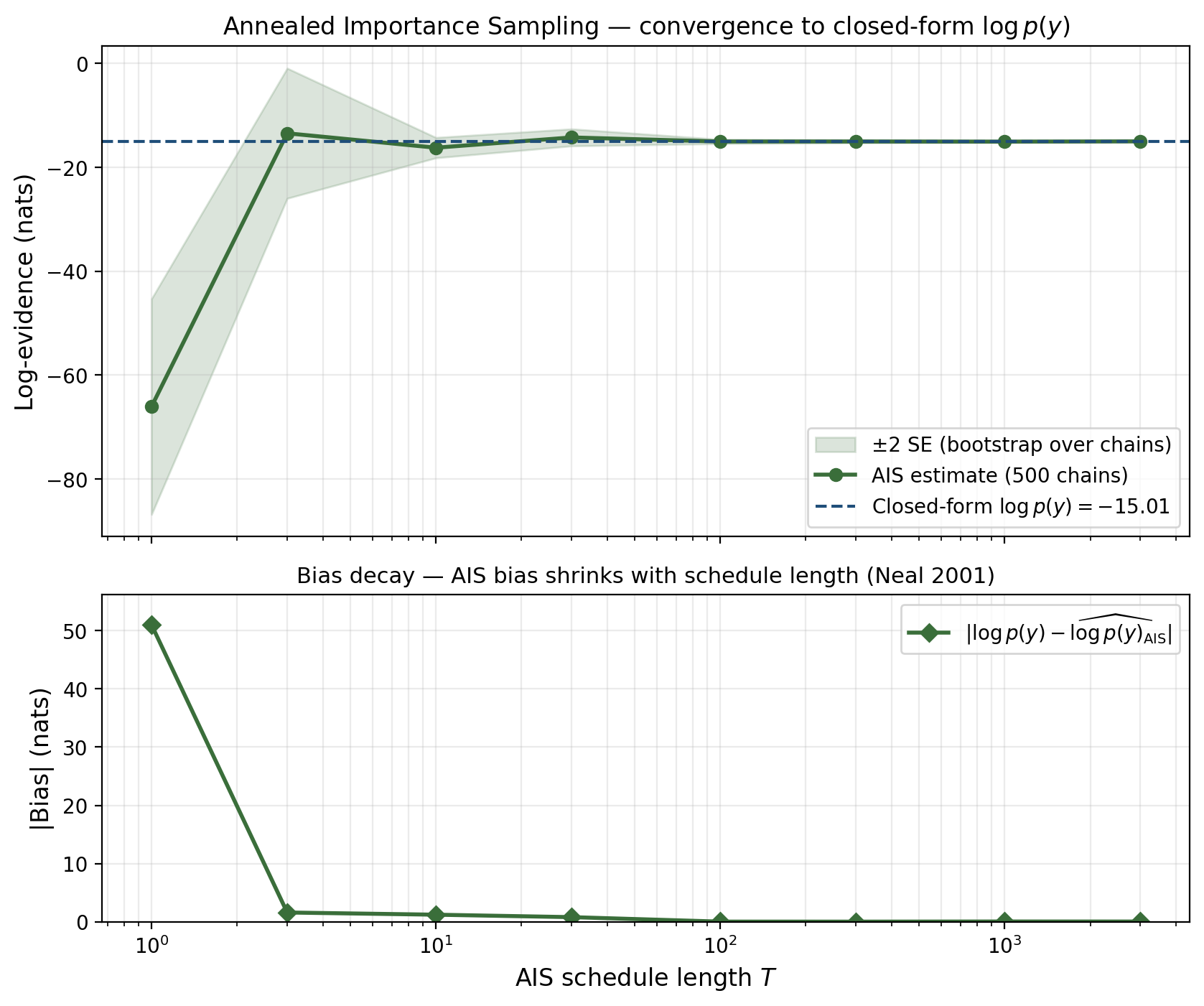
Compare to IWELBO from §8 on the same target: at $K = 1000$, IWELBO has measurable bias; AIS at $T = 100$ — a tenth the inner-loop count — is dramatically tighter. AIS is roughly two orders of magnitude more sample-efficient on this case. The reason: IWELBO does $K$ iid draws from a fixed proposal, so heavy importance-weight tails dominate. AIS does $T$ sequential draws through a schedule that gradually moves from prior to target.

Schedule design

A practical note: AIS’s sample efficiency depends on the schedule. Geometric schedules and adaptive schedules — Neal (2001) §6 — outperform linear when the posterior is much more concentrated than the prior. PyMC’s pm.sample_smc (Sequential Monte Carlo) is a related algorithm with adaptive scheduling.

For VBMS in production, the practical recipe is: use ELBO for the cheap first pass, use IWELBO at moderate $K$ to tighten when needed, and reach for AIS or SMC when Pareto-$\hat k$ flags problems or when the magnitude (not just the ranking) of the Bayes factor matters.

AIS schedule sweep on polynomial regression at d = 4

At T=1, AIS reduces to prior IS (high-variance). By T~50 the schedule has unfolded to land near closed-form.

d4

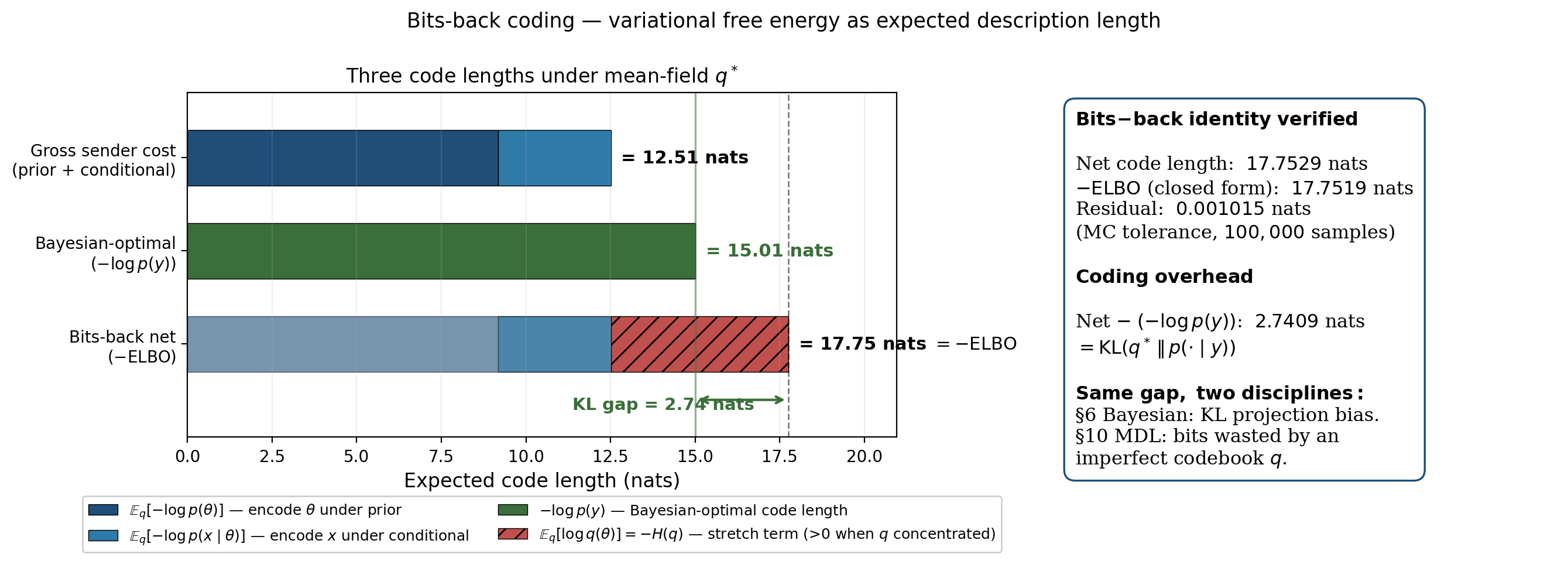
The MDL connection — variational free energy as bits-back coding

§§1–9 developed VBMS computationally. §10 changes the frame. We’ve been treating $\log p(y \mid M)$ as a probabilistic quantity — the marginal likelihood of the data under the model. It is also a coding-theoretic quantity — the optimal expected description length of the data under the model, in Shannon’s sense. The variational free energy $-\mathrm{ELBO}(q)$ is the analogous coding length under a constructive coding scheme that uses $q$ as a substitute for the true posterior. The gap between them — exactly the §6 KL projection bias — is the coding overhead the variational scheme pays for using an imperfect codebook.

This is the Minimum Description Length frame for VBMS. Hinton & van Camp (1993) introduced the bits-back coding protocol that makes the connection precise. Honkela & Valpola (2004) extended it to general variational Bayes.

The bits-back coding protocol

The protocol, with $q(\theta)$ a variational approximation to $p(\theta \mid y)$:

1. Sender draws $\theta \sim q(\theta)$. The randomness used to draw $\theta$ comes from an external source (an arithmetic-coded stream of auxiliary message bits). Drawing $\theta$ from $q$ uses up $-\log q(\theta)$ bits.
2. Sender encodes $\theta$ using a code based on the prior $p(\theta)$. Cost: $-\log p(\theta)$ bits.
3. Sender encodes $y$ using the conditional code $p(y \mid \theta)$. Cost: $-\log p(y \mid \theta)$ bits.
4. Receiver receives $\theta$ and $y$, decodes $\theta$ using $q$. Because both parties share $q$, the receiver can simulate the same arithmetic-decoding step, recovering the auxiliary message bits the sender used to draw $\theta$ — saving $-\log q(\theta)$ bits.

The net cost is the gross minus the bits back, in expectation under $\theta \sim q$.

The bits-back coding identity

The two halves of Theorem 8 say the same thing in two languages. Probabilistically: the variational free energy $-\mathrm{ELBO}(q)$ is at least the negative log-evidence, with the gap equal to the reverse-KL gap. Information-theoretically: the bits-back coding length is at least the Shannon-optimal code length, with the overhead equal to the same reverse-KL gap. The §6 KL projection bias is the bits-back coding overhead. Same object; two disciplines.

VBMS as MDL: shortest expected description length

The MDL frame for model selection: among candidate models $\{M_1, \ldots, M_K\}$, prefer the model that gives the shortest expected description length of the data. Under the optimal Bayesian code, this is the model with the highest $\log p(y \mid M)$. Under the bits-back protocol with a chosen variational family $\mathcal{Q}_M$ per model, this is the model with the highest $\mathrm{VBMS}(M)$ — the lowest variational free energy. In MDL language: VBMS is choosing the model whose variational coding scheme is most efficient.

This MDL frame matters for two reasons. First, it places VBMS within the broader minimum-description-length literature (Rissanen 1978, Grünwald 2007), connecting it to the BIC, MML, and other MDL-derived information criteria via shared coding-theoretic roots. Second, it suggests new model-selection criteria built on different coding protocols.

A coda on Hinton & van Camp’s original motivation: the 1993 paper introduced bits-back coding specifically for neural-network model compression — finding small networks whose weights have short bits-back description length, so that the network plus its weights compresses the training data well. Modern Bayesian neural network methods are direct descendants. The MDL connection is not just historical; it remains the motivating frame for several active areas of Bayesian deep learning.

Bits-back coding identity at d = 4

Theorem 8: bits-back net = −ELBO; the gap to the Shannon-optimal length is the §6 KL projection bias.

d4

Computational notes

The previous sections developed VBMS as a mathematical object. §11 is what the practitioner actually does at the keyboard.

The basic workflow

In PyMC, the canonical VBMS workflow looks like:

import pymc as pm
import arviz as az
import numpy as np

models = {"M_hier": build_hier_model(...), "M_pool": build_pool_model(...)}
elbos = {}
for name, model in models.items():
    with model:
        approx = pm.fit(n=30_000, method="advi", random_seed=0, progressbar=False)
    elbos[name] = -float(np.mean(approx.hist[-1000:]))  # last-1000-iter ELBO
log_BF = elbos["M_hier"] - elbos["M_pool"]

The output is a single scalar ELBO per model and a single log Bayes factor. Three immediate weaknesses: ADVI is non-convex, so random_seed=0 may have landed in a local optimum; the last-1000-iteration ELBO is a Monte Carlo estimate with non-trivial variance; and we have no diagnostic to tell us whether the variational posterior is a reasonable approximation.

Multiple restarts and max-ELBO selection

ADVI maximizes a non-convex objective. With one random seed, the result depends on initialization. The standard remedy is multiple random restarts, fitting ADVI from 5–20 different random seeds and selecting the maximum-ELBO restart as $\mathrm{VBMS}(M)$.

The ill-behaved cases:

• Variance collapse. Mean-field ADVI on heavy-tailed posteriors sometimes drives one or more variational variances to zero, giving a degenerate $q$ with $-\infty$ KL gap and an artificially huge “ELBO” that is meaningless.
• Mode collapse. On multimodal posteriors, ADVI restarts from different seeds can land in different modes with different ELBOs.
• Plateau ELBO. The ADVI optimization can plateau slightly below the true optimum.

A reasonable default: 10 restarts × 50,000 iterations, last-2000-iteration mean ELBO, max-ELBO selection across restarts.

The Pareto-$\hat k$ diagnostic

Yao, Vehtari, Simpson & Gelman (2018) proposed Pareto-smoothed importance sampling (PSIS) on the variational posterior as a diagnostic. The recipe: sample $S$ points $\theta_s \sim q^*(\theta)$, compute log importance weights $\log w_s = \log p(y, \theta_s) - \log q^*(\theta_s)$, fit a generalized Pareto distribution to the upper tail, and report the shape parameter $\hat k$.

The interpretation:

• $\hat k < 0.5$: the importance weights have finite variance, $q^*$ is a reliable approximation.
• $0.5 \le \hat k < 0.7$: the variance is finite but the tail is heavy enough that bias correction (IWELBO at moderate $K$) is recommended.
• $\hat k \ge 0.7$: the variance is infinite or the variational approximation has gone wrong; do not trust ELBO or IWELBO. Use AIS (§9) or full-rank VI.

ADVI versus full-rank versus structured VI

PyMC’s pm.fit accepts three method choices, in increasing order of expressiveness:

• method="advi" — mean-field Gaussian, $O(d)$ parameters. Fastest. Default.
• method="fullrank_advi" — full-rank Gaussian, $O(d^2)$ parameters. Captures linear correlation.
• method="svgd" or particle methods — non-parametric variational families.

For VBMS the choice matters because each method gives a different bias profile. A reasonable default: start with mean-field, escalate to full-rank when the $d$ is moderate ($d \le 100$) and Pareto-$\hat k$ is borderline. Beyond $d = 100$, structured VI with hand-designed factor groups (Hoffman & Blei 2015) is more sample-efficient than full-rank.

Hyperprior sensitivity

VBMS rankings can be sensitive to the strength of the prior at small $n$. The §4 Bishop GMM ARD example showed this in one direction: $\alpha_0 < 1$ drives ARD; $\alpha_0 \ge 1$ disables it. The remedy: report VBMS rankings under at least two prior strengths and flag any pair whose ranking flips between them as “prior-sensitive.”

Budget guidelines and escalation

A working budget hierarchy:

1. Mean-field ADVI, 10 restarts × 50K iter. ~1–10 seconds per model. First pass.
2. Pareto-$\hat k$ diagnostic. Always do this.
3. Full-rank ADVI if Pareto-$\hat k$ is borderline and $d \le 100$.
4. IWELBO at moderate $K$ ($K = 50$ to $K = 500$) if ranking magnitudes matter.
5. AIS or SMC if Pareto-$\hat k$ is $\ge 0.7$, if multimodality is suspected, or if the magnitude of the Bayes factor matters.
6. Run all of the above and compare if the comparison is high-stakes.

VBMS in modern ML

The §1–§11 development has been deliberately mathematical. We close the technical part of the topic with a brief tour of where VBMS shows up in modern machine learning practice.

BNN width and depth selection. A Bayesian neural network is a parametric model whose architecture is itself a model-selection choice. VBMS gives a fast first-pass ranking: fit ADVI on each architecture, take ELBO differences, rank. The §7 ranking-preservation criterion governs when this is reliable. The Bayesian Neural Networks topic develops the full BNN-VBMS workflow, including the MC-dropout-as-VI shortcut.

Neural architecture search. VBMS scales the BNN-width-selection idea to the full NAS problem: enumerate architectures, fit ADVI on each, rank by VBMS, take the top-$k$ for full HMC re-ranking, deploy the winner. Modern NAS literature has converged on this two-stage pattern (VBMS-style fast oracle plus expensive re-ranking).

Sparse Bayesian priors. Choosing among horseshoe, regularized horseshoe, spike-and-slab, R2-D2 priors on a specific dataset is a model-selection problem. VBMS over the hyperprior choices ranks them by ELBO. The mean-field bias is non-trivial here — sparse priors typically have heavy-tailed posteriors that mean-field underestimates — so full-rank or flow VI is the right tool. Sparse Bayesian Priors develops this in detail, with §11 specializing the VBMS escalation hierarchy to the four-prior menu and §6 working through the funnel pathology that makes naive HMC fail on the horseshoe.

Singular models and Watanabe’s WAIC. The §3 BIC asymptotic equivalence theorem required the Hessian to be positive definite at the MAP, which excludes singular models — mixture models, neural networks, and hidden Markov models. For these, the BIC’s $-(d/2) \log n$ penalty is wrong, and Watanabe’s (2010) WBIC and WAIC replace it with corrections derived from singular learning theory. The variational analog — VBMS for singular models — is an open research question.

Amortized variational inference. When VBMS is used inside an iterative algorithm, the cost of fitting a fresh ADVI from scratch for each candidate model becomes the bottleneck. Amortized inference — training an inference network that maps from data to variational parameters — replaces the per-task optimization with a forward pass. The planned Meta-Learning (coming soon) topic develops the connection.

Connections and limits

We’ve developed VBMS as a self-contained model-selection tool. What remains is to place the topic in its broader context — to show where VBMS sits in the landscape of model-selection methodology, what it does well, what it does badly, and which tool to reach for when VBMS is the wrong answer.

formalML topology

VBMS depends on five formalML topics as substrates and informs at least four planned T5 topics directly.

Backward dependencies. Variational Inference is the substrate — VBMS is variational inference applied to the marginal-likelihood integral. KL Divergence sits underneath — the §6 reverse-KL projection picture and the §7 mode-seeking distinction depend on the KL-divergence topic’s f-divergence framework. Minimum Description Length is the substrate of §10 — the bits-back coding identity discharges the curriculum-graph prereq edge directly. Bayesian Neural Networks §3 develops the Laplace approximation at full depth. Gradient Descent §4 develops the ADVI optimizer that §11 takes as a black box.

Forward dependencies. Several planned T5 topics build on VBMS. Sparse Bayesian Priors uses VBMS to rank horseshoe / regularized horseshoe / spike-and-slab / R2-D2 priors on a fixed dataset, with PSIS Pareto-$\hat k$ as the gating diagnostic. Meta-Learning (coming soon) develops amortized variational inference. Stacking and Predictive Ensembles covers the M-open alternative to VBMS.

The M-closed / M-complete / M-open framework

The Bernardo & Smith (1994) framework distinguishes three regimes for Bayesian model comparison:

• M-closed — the true data-generating process is one of the candidate models. This is the regime VBMS, BIC, and BMA all assume.
• M-complete — the true data-generating process is outside the candidate set, but well-approximated by some convex combination. The asymptotic story is similar to M-closed.
• M-open — the true data-generating process is genuinely outside the candidate set, and no convex combination of candidates is a good approximation. The right tool is stacking (Yao et al. 2018b).

For a topic on VBMS, M-closed is the assumed regime.

Honest limits

Three structural limits of VBMS:

ELBO is not a model-quality metric. When the same model is fit multiple times with different random seeds, the ELBO can vary by 0.1 to several nats — this is optimization variance, not statistical evidence.

Mode-seeking on multimodal posteriors. Reverse-KL projection is mode-seeking; on multimodal posteriors with $K$ distinct modes, mean-field VB collapses to a single mode and the resulting ELBO is missing $-\log K$ nats of probability mass. For physically meaningful multimodality, the ELBO bias is real and rankings can be catastrophically wrong.

The bias is a permanent feature, not an artifact. §6 made the geometric statement: for any parametric variational family that does not contain the posterior, the bias is non-zero. No engineering trick eliminates it — only growing the family does. For VBMS in production, the §11 escalation hierarchy is needed; bias correction is not a formality but a working necessity for high-stakes comparisons.

Alternatives: when to reach for which

Five major alternatives to VBMS for model selection:

Bayesian Information Criterion (BIC, Schwarz 1978). The leading-order Laplace approximation to $\log p(y \mid M)$ as $n \to \infty$. Reach for it when: $n$ is large, the model is regular, the data are iid, and the candidate set is M-closed. Don’t reach for it when: $n$ is small, the model is singular, or the comparison is in M-open.

Akaike Information Criterion (AIC, Akaike 1974). A predictive-accuracy criterion with a $-2 \log L(\hat\theta_{\mathrm{MLE}}) + 2d$ form. Reach for it when: the goal is predictive performance rather than identifying the true model.

Widely Applicable Information Criterion (WAIC, Watanabe 2010). A predictive-accuracy criterion that handles singular models. Reach for it when: the model is singular; MCMC samples are available; the goal is predictive accuracy.

Pareto-smoothed importance-sampled leave-one-out cross-validation (PSIS-LOO, Vehtari et al. 2017). Approximate LOO via importance sampling on posterior draws. Reach for it when: the goal is small-data predictive performance; MCMC samples are available.

Bayesian Model Averaging (BMA, Hoeting et al. 1999). Rather than picking a single model, average the predictions of all candidate models weighted by their posterior model probabilities. Reach for it when: M-closed assumption holds; the goal is predictive performance under model uncertainty.

Stacking (Yao et al. 2018b). Average predictive distributions from candidate models via weights chosen to optimize cross-validated predictive accuracy. Reach for it when: M-open assumption holds. The Stacking and Predictive Ensembles topic develops the framework in detail.

A decision tree, simplified:

• M-closed and want to identify the true model → VBMS or BIC for ranking, plus PSIS-LOO for confirmation.
• M-closed and want predictive performance → BMA, with VBMS or marginal-likelihood-based weights.
• M-complete and want predictive performance → BMA or stacking; the choice depends on how close to M-closed the data are.
• M-open → stacking. Don’t use VBMS, BMA, or BIC.
• Singular models (mixtures, NNs, HMMs) → WAIC for ranking; PSIS-LOO for predictive accuracy. VBMS is OK if you’re careful about Pareto-$\hat k$.
• Small data with sensitivity to hyperpriors → PSIS-LOO with sensitivity sweeps; VBMS with hyperprior sensitivity analysis.
• Large-scale exploration (NAS, hyperparameter grids) → VBMS for the first pass; AIS or PSIS-LOO for top-$k$ confirmation.

VBMS sits in the “fast, biased, useful for M-closed and M-complete” niche. It is not the right tool for M-open work or for high-stakes singular-model comparisons. Knowing where it fits and where it doesn’t is most of the value of the topic.

Closing remarks

Variational inference replaced the intractable evidence integral with an optimization. Variational Bayes for model selection took that optimization one step further and turned it into a model-comparison criterion — fast, biased, with bias structure characterizable through the §6 reverse-KL projection picture and the §7 Wang–Blei consistency theorem. The topic’s central claim, restated: the ELBO is not a wrong estimator of the log-evidence but a biased one with known mechanism, and that mechanism is informative enough that VBMS rankings agree with closed-form rankings in most regimes practitioners care about.

The right way to use VBMS, in one sentence: fit ADVI for each candidate model with multiple restarts; compute Pareto-$\hat k$ on the variational posteriors; report VBMS rankings if Pareto-$\hat k$ is small and the comparison is M-closed; escalate to IWELBO, AIS, or stacking when these conditions don’t hold.

VBMS is one tool. The topic was about understanding it well — its mechanics, its bias, its scope, and its place in the larger model-selection landscape.