Gradient Descent & Convergence
The workhorse of continuous optimization: convergence rates under smoothness and strong convexity, acceleration, coordinate descent, mirror descent, and stochastic variants
Overview & Motivation
In Convex Analysis we established the geometric and analytic infrastructure that makes optimization tractable: convex sets are closed under line segments, convex functions have a single global minimum, and smooth convex functions admit tangent-line lower bounds. That machinery tells us what to optimize but not how. This topic is about the how.
Gradient descent is the simplest first-order algorithm for unconstrained minimization, and arguably the most important. The idea is disarmingly simple: to minimize , start at an initial guess and repeatedly take steps in the direction that decreases fastest — the negative gradient . Each step replaces the function by its local linear approximation and moves to where that approximation is most favorable.
What makes gradient descent remarkable is not the algorithm itself but the convergence theory that governs it. With the right assumptions — smoothness, convexity, and sometimes strong convexity — we can prove exactly how fast the iterates approach the optimum, and these rates turn out to be tight: no first-order method can do better in the worst case (at least without acceleration).
What We Cover
- The Gradient Descent Algorithm — the update rule and its geometric interpretation as steepest descent.
- Smoothness & the Descent Lemma — how -smoothness provides a quadratic upper bound that guarantees progress at each step.
- Convergence for Convex Functions — the sublinear rate, proven via telescoping.
- Strong Convexity & Linear Convergence — the condition number and the geometric rate .
- Step Size Selection — fixed, exact line search, and Armijo backtracking.
- Nesterov Accelerated Gradient — the momentum trick that achieves the optimal rate.
- Coordinate Descent — updating one variable at a time, and when that beats full-gradient steps.
- Mirror Descent & Bregman Divergence — generalizing Euclidean geometry for constrained domains.
- Stochastic Gradient Descent — noisy gradients, mini-batches, and decreasing step sizes.
- Computational Notes — NumPy implementations and convergence diagnostics.
The Gradient Descent Algorithm
The gradient points in the direction of steepest increase of at . To decrease , we walk in the opposite direction.
Definition 1 (Gradient Descent Update).
Given a differentiable function , a starting point , and a step size (learning rate) , the gradient descent algorithm generates iterates
The iteration terminates when falls below a chosen tolerance, or after a fixed budget of steps.
Geometrically, each iterate replaces by its first-order Taylor approximation and moves in the direction that decreases this linear model fastest. The step size controls how far we trust the linear approximation — too large and we overshoot; too small and progress is glacially slow.
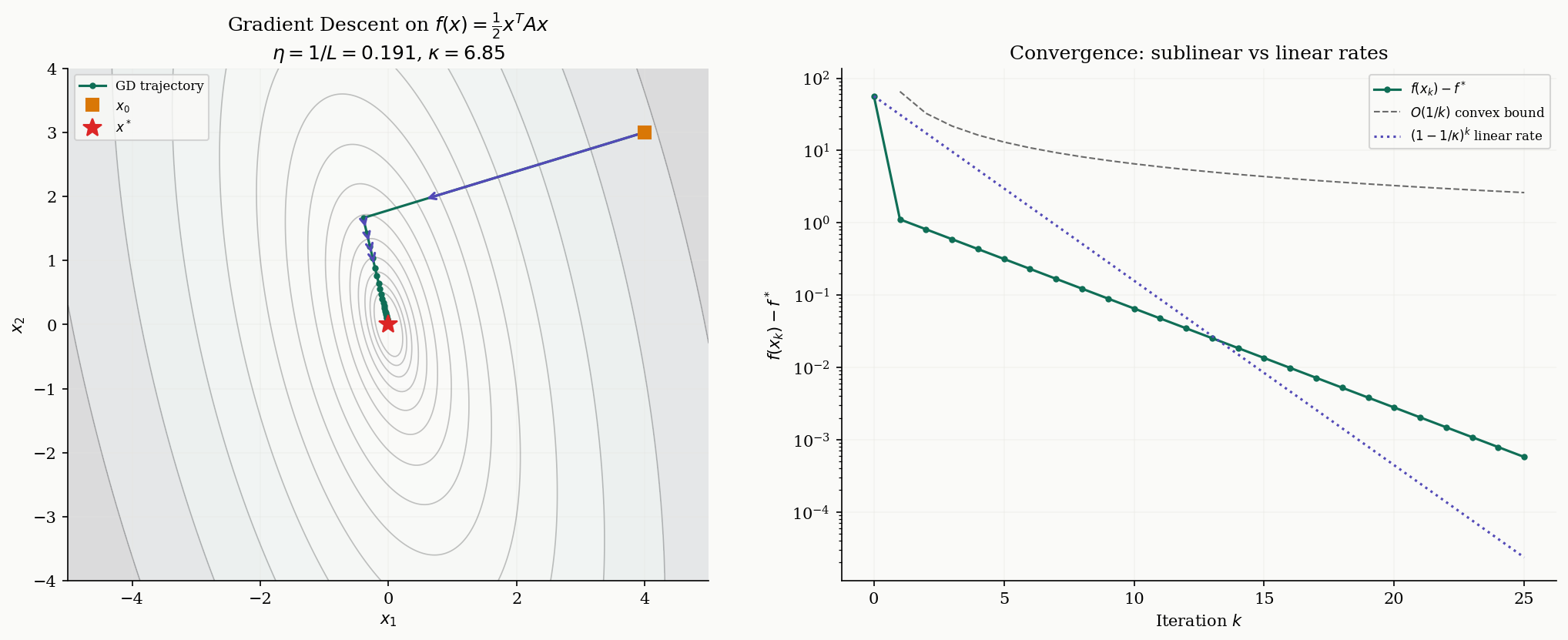
For a quadratic with symmetric positive definite, the gradient is and the update simplifies to . The convergence behavior of this linear map is entirely determined by the eigenvalues of : convergence requires for every eigenvalue , which means must lie in .
Smoothness & the Descent Lemma
The key to analyzing gradient descent is smoothness — a Lipschitz condition on the gradient that provides a global quadratic upper bound on .
Definition 2 (L-Smoothness).
A differentiable function is -smooth (or has -Lipschitz continuous gradient) if
The constant is the smoothness parameter. For twice-differentiable functions, -smoothness is equivalent to for all — that is, the Hessian’s eigenvalues are bounded above by .
Smoothness says the gradient cannot change too fast. This is exactly the condition that allows us to guarantee progress at each gradient step: if the gradient doesn’t change too fast between and , then the decrease predicted by the linear approximation actually holds (up to a quadratic correction).
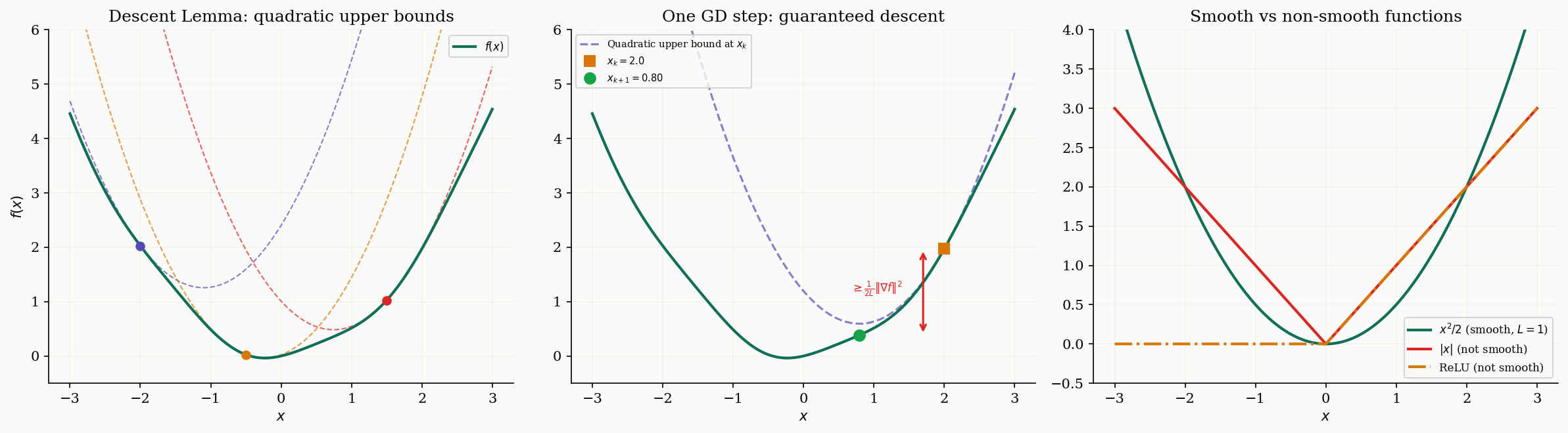
Theorem 1 (The Descent Lemma).
If is -smooth, then for all :
In particular, taking a gradient step yields the guaranteed decrease:
Proof.
By the fundamental theorem of calculus,
Adding and subtracting :
By Cauchy–Schwarz and the -Lipschitz condition on the gradient:
Integrating from to :
For the guaranteed decrease, substitute :
∎
The Descent Lemma tells us that at each point , the function is sandwiched between a linear lower bound (from convexity, if is convex) and a quadratic upper bound (from -smoothness). The gradient step minimizes the upper bound exactly, and the decrease is proportional to .
Convergence for Convex Functions
Armed with the Descent Lemma, we can prove the first convergence result. For a convex, -smooth function, gradient descent with step size achieves an rate — sublinear, but dimension-free.
Theorem 2 (Convergence for Convex + L-Smooth Functions).
Let be convex and -smooth, and let be a minimizer of . Then gradient descent with step size satisfies:
Proof.
From the Descent Lemma, each step guarantees:
Since is convex, the first-order condition gives us , which rearranges to:
We will use a different approach that yields the tightest bound. Consider the distance to the optimum:
Rearranging and using the convexity inequality :
From (1), . Since , we get:
Now telescope: sum both sides from to :
Since is non-increasing (by the Descent Lemma), , giving:
∎
The rate tells us that to reach -accuracy, we need iterations. This depends on the initial distance to the optimum but — crucially — not on the dimension .
Strong Convexity & Linear Convergence
The rate is slow. If we strengthen our assumption from plain convexity to strong convexity, the rate improves dramatically from sublinear to linear (i.e., geometric).
Definition 3 (μ-Strong Convexity).
A differentiable function is -strongly convex (with ) if for all :
Equivalently, is convex, or for all .
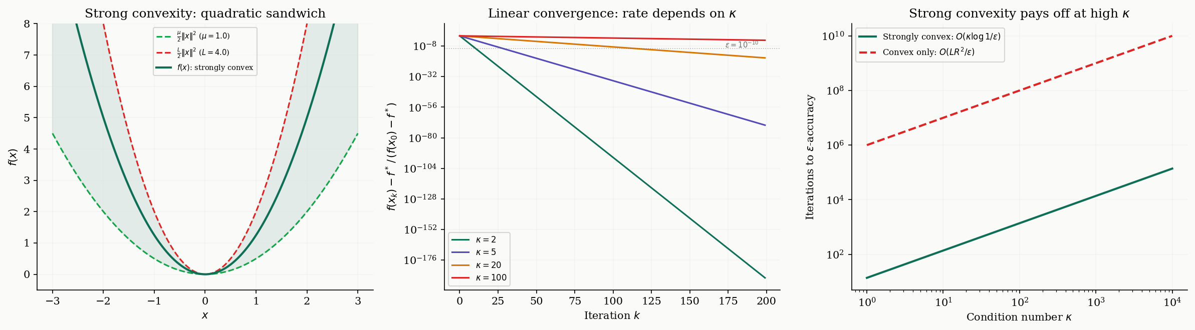
Strong convexity says that curves upward at least as fast as a quadratic with parameter . Together with -smoothness, this gives a “quadratic sandwich”:
Definition 4 (Condition Number).
For an -smooth, -strongly convex function, the condition number is:
For a quadratic with symmetric positive definite, , , and equals the spectral condition number of (see The Spectral Theorem). For least-squares problems , the relevant condition number is from the SVD.
Theorem 3 (Linear Convergence Under Strong Convexity).
Let be -smooth and -strongly convex with condition number . Then gradient descent with step size satisfies:
Proof.
The Descent Lemma gives . Subtracting :
We need a lower bound on in terms of . Strong convexity gives us a key inequality (the Polyak–Łojasiewicz condition):
To see why: by -strong convexity, for any ,
Minimizing the right side over (a quadratic in ), the minimum is achieved at and equals . Since :
which rearranges to .
Substituting into (3):
Applying this recursion times completes the proof.
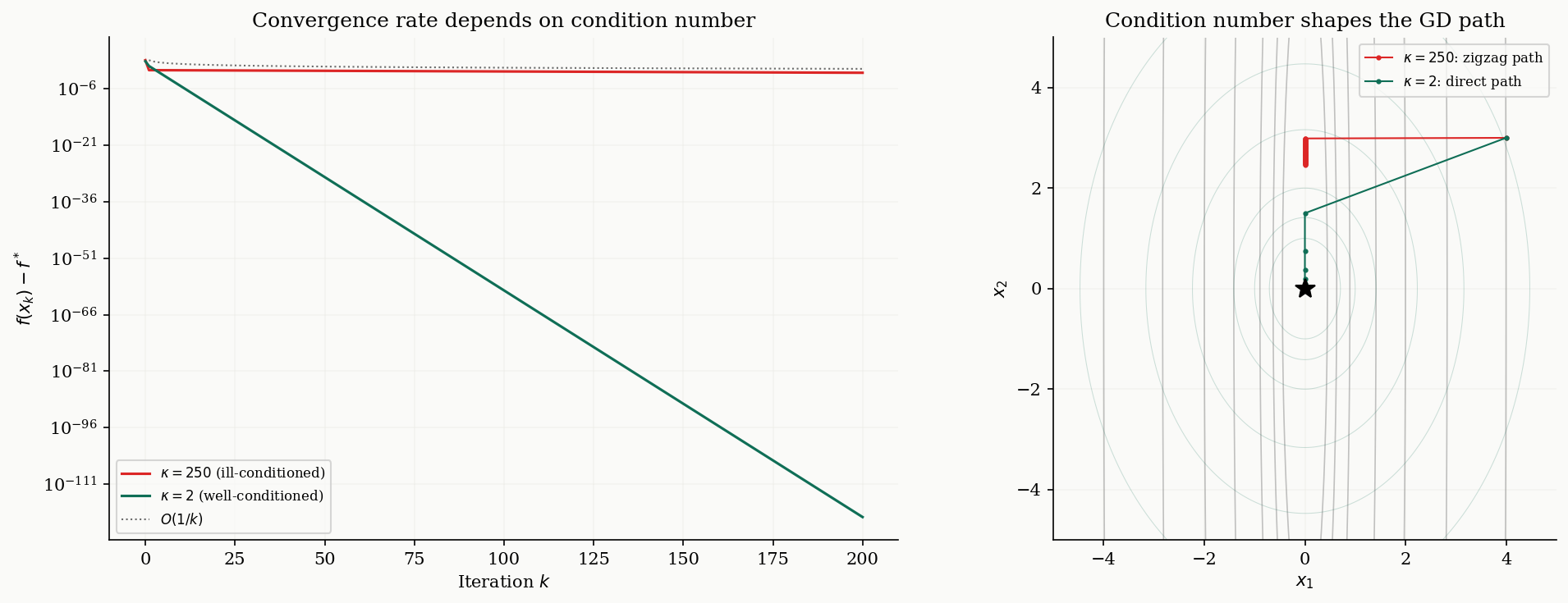
∎The linear rate means decreases at a constant rate per iteration — the convergence plot is a straight line on a log scale. To reach -accuracy, we need iterations. The dependence on is logarithmic (much better than the for the convex case), but the price is a linear dependence on . Ill-conditioned problems (large ) converge slowly because the contours are highly elongated ellipses, and gradient descent zigzags across the narrow valley.
Step Size Selection
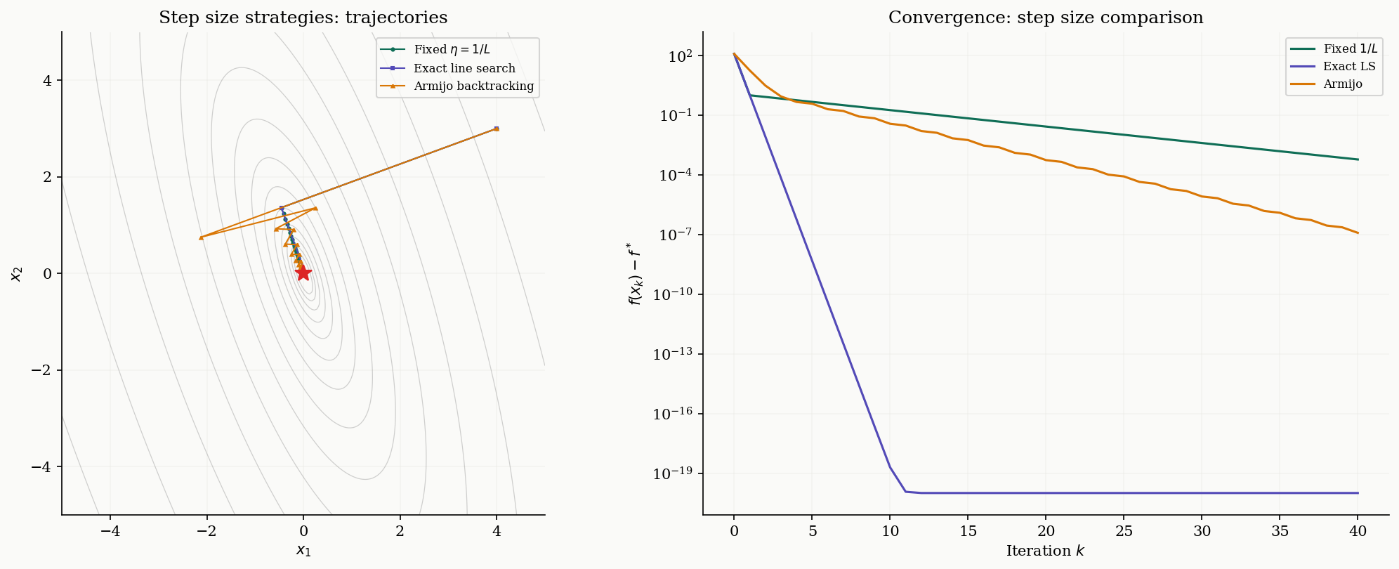
So far we’ve used the fixed step size , which requires knowing in advance. In practice, there are several strategies.
Exact line search
This strategy chooses the step size that minimizes along the gradient direction:
For a quadratic , this has a closed-form solution:
Exact line search always converges at least as fast as fixed step size but is usually impractical for non-quadratic objectives.
Definition 5 (Armijo Sufficient Decrease Condition).
Given parameters (typically ) and backtracking factor (typically ), the Armijo backtracking line search starts with and repeatedly sets until:
This is the sufficient decrease (Armijo) condition: it requires a decrease proportional to the step size and the squared gradient norm.
Proposition 1 (Armijo Termination).
If is -smooth, Armijo backtracking with any and terminates in a finite number of halvings. Specifically, any satisfies the Armijo condition, so the search terminates with .
Proof.
From the Descent Lemma, for any :
For the Armijo condition to hold, we need , which simplifies to . Since the search reduces by factors of , it will find such an within halvings.
∎
Nesterov Accelerated Gradient
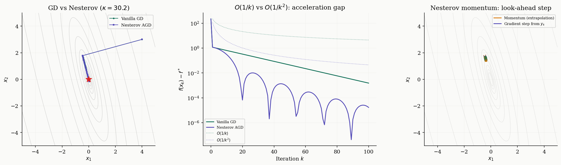
Gradient descent with step size converges at rate for convex functions. Can we do better? Nesterov showed in 1983 that the answer is yes — and that is optimal among all first-order methods.
Definition 6 (Nesterov Accelerated Gradient).
The Nesterov accelerated gradient (NAG) method maintains a sequence of iterates and extrapolation points :
where the sequence satisfies and .
The critical difference from vanilla gradient descent: the gradient is evaluated at the extrapolated point , not at the current iterate . The extrapolation step adds a “momentum” term — it looks ahead in the direction the iterates have been moving, then computes the gradient at that look-ahead point.
Theorem 4 (Nesterov's Optimal Rate).
Let be convex and -smooth. Then the Nesterov accelerated gradient method satisfies:
This is an rate, which is optimal among all first-order methods that access only through gradient evaluations (Nesterov, 1983).
We state this theorem without proof — the proof requires a carefully constructed Lyapunov function argument that we refer the reader to Nesterov’s original paper.
Remark (Why O(1/k²) Is Optimal).
Nesterov also proved a matching lower bound: for any first-order method that generates iterates in the Krylov subspace , there exists an -smooth convex function for which . The accelerated gradient method achieves this lower bound and is therefore optimal in this class. This is one of the rare results in optimization where we have matching upper and lower bounds.
Coordinate Descent
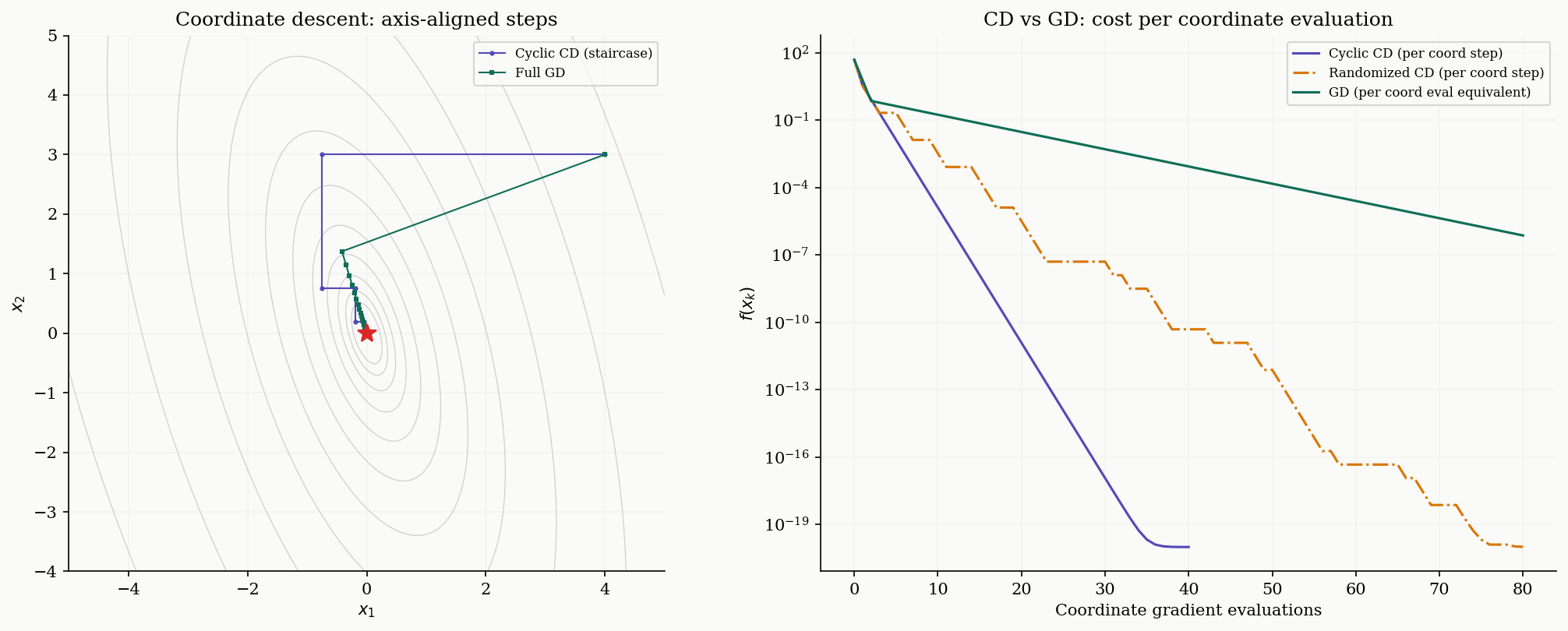
Instead of computing the full gradient , coordinate descent updates one coordinate at a time. This is attractive when is large and computing a single partial derivative is cheap.
Definition 7 (Coordinate Descent).
Cyclic coordinate descent updates coordinates in order :
where is the smoothness constant along coordinate . For , this is .
Randomized coordinate descent selects uniformly at random at each step.
The characteristic visual signature of coordinate descent is the “staircase” pattern on contour plots: each step moves along a coordinate axis, creating axis-aligned zigzags. Compare this with gradient descent, which moves along the gradient direction (which is generally not axis-aligned).
Theorem 5 (Randomized Coordinate Descent Convergence).
Let be convex with coordinate-wise smoothness constants . Then randomized coordinate descent with step sizes satisfies:
where .
Proof.
At each step, we select coordinate uniformly at random and update . The coordinate-wise Descent Lemma gives:
Taking expectations over the random coordinate:
The rest follows the same telescoping argument as Theorem 2, with replaced by .
∎Remark (When Coordinate Descent Wins).
The rate looks worse than GD’s , but each CD step costs gradient component while each GD step costs . When measured in coordinate gradient evaluations, the rates are comparable. CD wins when: (1) the function has separable or block-separable structure, (2) is very large and computing the full gradient is expensive, or (3) the coordinate-wise smoothness constants vary widely (some coordinates are much smoother than others).
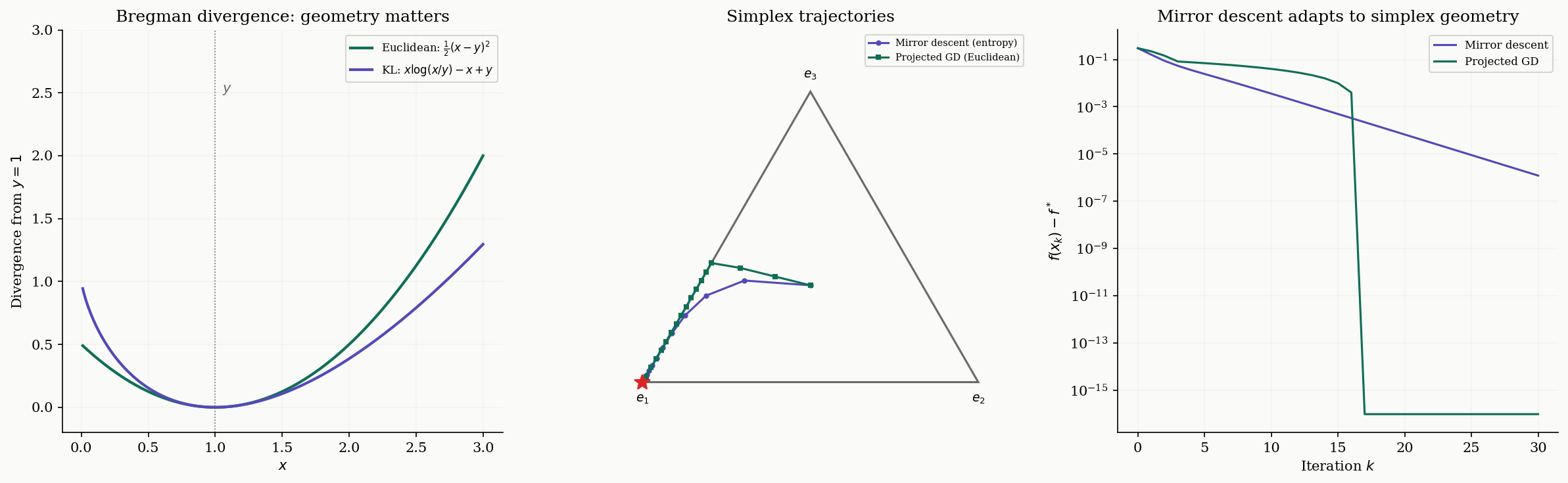
Mirror Descent & Bregman Divergence
Gradient descent implicitly uses Euclidean distance to measure progress: the update can be written as
But Euclidean distance is not always the right geometry. When optimizing over the probability simplex , the Euclidean distance treats points near the boundary the same as interior points, which is wasteful — near a vertex, most directions leave the simplex. Mirror descent replaces with a Bregman divergence matched to the geometry of the domain.
Definition 8 (Bregman Divergence).
Given a strictly convex, differentiable function (the mirror map), the Bregman divergence is:
This measures the gap between and its first-order Taylor approximation at . By strict convexity, with equality iff .
When , the Bregman divergence reduces to — ordinary Euclidean distance. When (the negative entropy), the Bregman divergence is the KL divergence .
Definition 9 (Mirror Descent).
The mirror descent update with mirror map and step size is:
When and is the simplex, this yields the exponentiated gradient update:
The exponentiated gradient update naturally maintains positivity and the simplex constraint without explicit projection. Mirror descent with negative entropy is the natural algorithm for the simplex: its iterates curve along the simplex boundary rather than cutting through the interior in straight lines.
Proposition 2 (Mirror Descent Convergence).
Let be convex and -Lipschitz ( for all ), and let be -strongly convex with respect to a norm . Then mirror descent with step size (where ) satisfies:
Proof.
From the mirror descent update definition and the three-point identity for Bregman divergence:
By convexity, . Summing from to , the Bregman terms telescope to . Using and optimizing gives the result.
∎The connection to Proximal Methods is deep: mirror descent is a special case of the proximal point algorithm with Bregman divergence replacing Euclidean distance. Proximal operators generalize the gradient step to handle non-smooth regularizers like the norm.
Stochastic Gradient Descent
In machine learning, the objective is often an average over a large dataset: . Computing the full gradient requires gradient evaluations per step, which is expensive when is large. Stochastic gradient descent (SGD) replaces the full gradient with a noisy but unbiased estimate.
Definition 10 (Stochastic Gradient Descent).
Given an unbiased gradient estimator satisfying and , stochastic gradient descent performs:
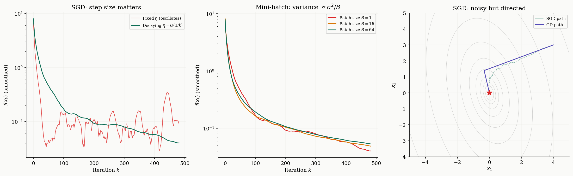
The mini-batch variant averages independent samples: , reducing variance to .
The step size schedule is crucial. With a fixed step size , SGD converges to a neighborhood of the optimum but cannot reach it — the noise prevents the iterates from settling down. A decreasing schedule allows convergence to the exact optimum, at the cost of slower progress.
Theorem 6 (SGD Convergence).
Let be convex and -smooth, and let the gradient estimator have bounded variance . Then:
Fixed step size :
Optimizing gives an rate.
Decreasing step size : SGD converges to the optimum at rate for strongly convex objectives.
Proof.
From the smoothness of and the SGD update:
Since (bias-variance decomposition):
For , the term . Rearranging and summing over gives the stated bound. The key tension: the first term decreases with (more iterations help), but the second term remains constant for fixed . Decreasing eliminates the residual at the cost of slower convergence.
∎
Computational Notes
Here we collect practical implementations. The gradient_descent function below supports fixed step size and Armijo backtracking, and returns the full convergence history for diagnostic plotting.
def gradient_descent(f, grad_f, x0, eta=None, L=None, tol=1e-8, max_iter=1000,
                     line_search='fixed'):
    """
    General-purpose gradient descent.

    Parameters
    ----------
    f : callable — objective function
    grad_f : callable — gradient of f
    x0 : ndarray — initial point
    eta : float — fixed step size (required if line_search='fixed')
    L : float — Lipschitz constant; used for eta=1/L if eta not given
    tol : float — gradient norm tolerance
    max_iter : int — iteration budget
    line_search : str — 'fixed' or 'armijo'

    Returns
    -------
    dict with keys 'x', 'f_vals', 'grad_norms', 'trajectory', 'n_iter'
    """
    if eta is None and L is not None:
        eta = 1.0 / L

    x = x0.copy()
    f_vals = [f(x)]
    grad_norms = [np.linalg.norm(grad_f(x))]
    trajectory = [x.copy()]

    for k in range(max_iter):
        g = grad_f(x)
        if np.linalg.norm(g) < tol:
            break

        if line_search == 'armijo':
            step = armijo_backtracking(f, grad_f, x, -g)
        else:
            step = eta

        x = x - step * g
        f_vals.append(f(x))
        grad_norms.append(np.linalg.norm(grad_f(x)))
        trajectory.append(x.copy())

    return {
        'x': x,
        'f_vals': np.array(f_vals),
        'grad_norms': np.array(grad_norms),
        'trajectory': np.array(trajectory),
        'n_iter': len(f_vals) - 1
    }
The Armijo backtracking function:
def armijo_backtracking(f, grad_f, x, d, alpha0=1.0, beta=0.5, c=1e-4, max_iter=50):
    """Armijo backtracking line search."""
    alpha = alpha0
    fx = f(x)
    gx = grad_f(x)
    for _ in range(max_iter):
        if f(x + alpha * d) <= fx + c * alpha * (gx @ d):
            return alpha
        alpha *= beta
    return alpha
Nesterov accelerated gradient:
def nesterov_gd(A, x0, n_iter=100):
    """Nesterov accelerated gradient for f(x) = 0.5 x^T A x."""
    L = eigvalsh(A)[-1]
    eta = 1.0 / L
    x, y = x0.copy(), x0.copy()
    traj = [x0.copy()]
    t = 1.0
    for k in range(n_iter):
        x_new = y - eta * (A @ y)
        t_new = (1 + np.sqrt(1 + 4 * t**2)) / 2
        y = x_new + ((t - 1) / t_new) * (x_new - x)
        x, t = x_new, t_new
        traj.append(x.copy())
    return np.array(traj)
Cyclic coordinate descent:
def cyclic_cd(A, x0, n_iter=50):
    """Cyclic coordinate descent for f(x) = 0.5 x^T A x."""
    x = x0.copy()
    traj = [x.copy()]
    for _ in range(n_iter):
        for i in range(len(x0)):
            grad_i = A[i, :] @ x
            x[i] -= grad_i / A[i, i]
            traj.append(x.copy())
    return np.array(traj)
Mirror descent on the simplex (exponentiated gradient):
def mirror_descent_simplex(grad_f, x0, eta, n_iter=50):
    """Mirror descent with neg-entropy on the probability simplex."""
    x = x0.copy()
    traj = [x.copy()]
    for _ in range(n_iter):
        g = grad_f(x)
        x_new = x * np.exp(-eta * g)
        x_new /= x_new.sum()
        x = x_new
        traj.append(x.copy())
    return np.array(traj)
SGD with mini-batch averaging:
def sgd_minibatch(A, x0, eta_schedule, noise_std=1.0, batch_size=1,
n_iter=500, seed=42):
"""SGD with Gaussian gradient noise and mini-batch averaging."""
rng = np.random.RandomState(seed)
x = x0.copy()
traj = [x.copy()]
for k in range(n_iter):
eta = eta_schedule(k)
true_grad = A @ x
noise = rng.randn(batch_size, len(x)) * noise_std
x = x - eta * (true_grad + noise.mean(axis=0))
traj.append(x.copy())
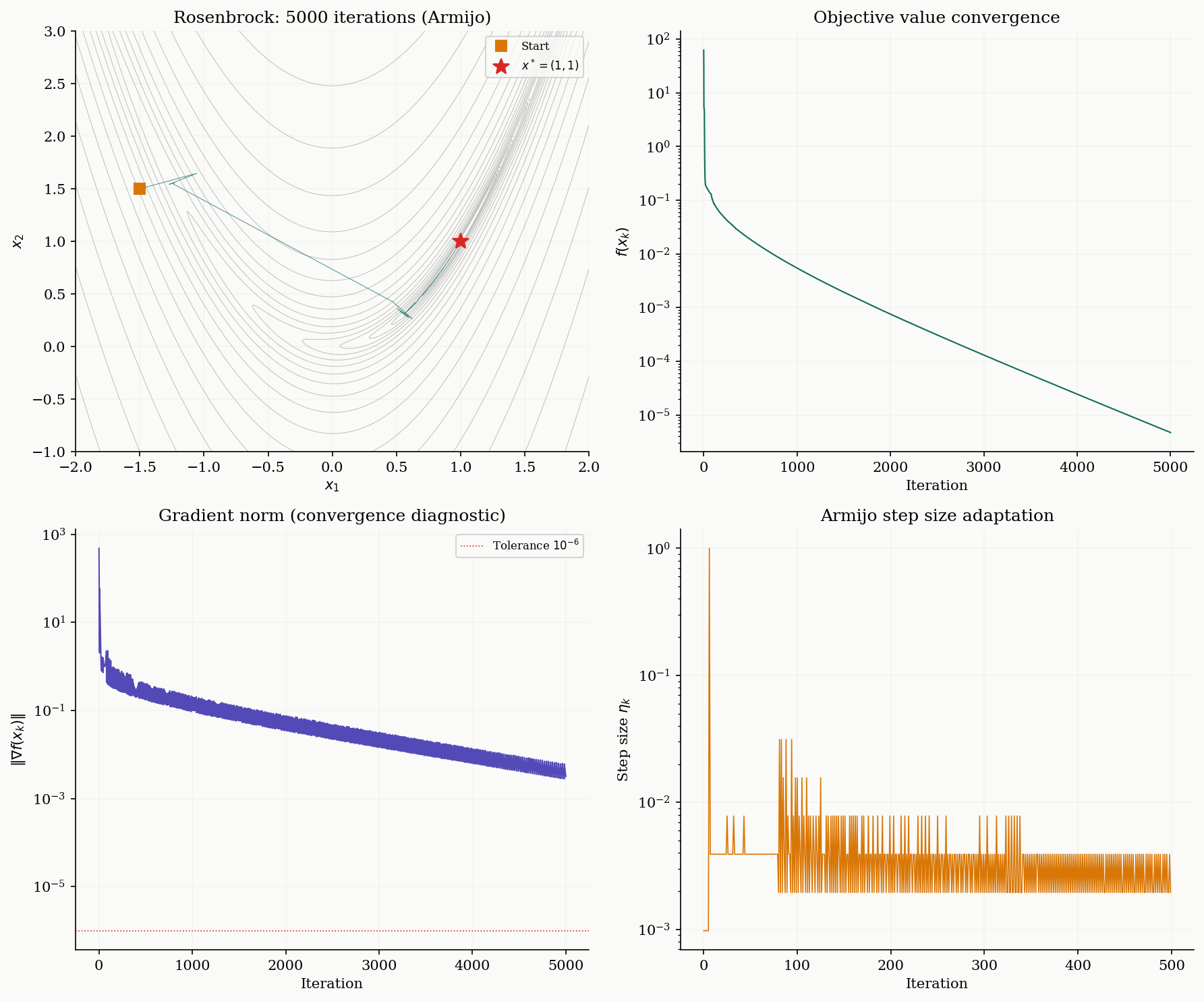
return np.array(traj)Convergence diagnostics. When running gradient descent in practice, monitor four quantities: (1) the objective value , which should decrease monotonically for deterministic GD; (2) the gradient norm , which indicates proximity to a stationary point; (3) the step size history (if using backtracking); and (4) the trajectory in parameter space (for low-dimensional problems).
Connections & Further Reading
Gradient descent sits at the center of the Optimization track, building on convex analysis and connecting forward to proximal methods and duality.
| Topic | Connection |
|---|---|
| Convex Analysis | Every convergence proof here relies on convexity and smoothness established in Convex Analysis. The Descent Lemma is the -smooth analogue of the first-order convexity condition; strong convexity provides the quadratic lower bound that yields linear convergence. |
| The Spectral Theorem | The condition number for quadratics equals of the Hessian. Ill-conditioned Hessians (large eigenvalue spread) cause the zigzag behavior that slows gradient descent. |
| Singular Value Decomposition | For least-squares problems , the condition number of governs GD convergence. The SVD reveals this as , connecting linear algebra to optimization dynamics. |
| Proximal Methods | Mirror descent generalizes to proximal operators: . Proximal gradient descent handles composite objectives where is non-smooth but has a cheap proximal operator (e.g., regularization). |
| Lagrangian Duality & KKT | Constrained optimization extends the unconstrained theory here. The KKT conditions generalize “gradient equals zero” to include constraints, and dual gradient descent operates on the Lagrangian dual function. |
| Quantile Regression | The smoothed-check-loss + Nesterov accelerated gradient solver in QR’s in-browser viz components is a direct application of Moreau-envelope smoothing — the non-smooth pinball loss is replaced by , which has -Lipschitz gradient (so AGD’s rate applies) and recovers as . |
The Optimization Track
Convex Analysis
    ├── Gradient Descent & Convergence (this topic)
    │       └── Proximal Methods
    └── Lagrangian Duality & KKT
Connections
- Every convergence proof in this topic relies on convexity and smoothness properties established in Convex Analysis. The Descent Lemma is the L-smooth analogue of the first-order convexity condition; strong convexity provides the quadratic lower bound that yields linear convergence. convex-analysis
- The condition number κ = L/μ for quadratic objectives equals the ratio of extreme eigenvalues of the Hessian. The Spectral Theorem provides the eigendecomposition that makes this concrete: ill-conditioned Hessians (large eigenvalue spread) cause the zigzag behavior that slows gradient descent. spectral-theorem
- For least-squares problems min ||Ax - b||², the condition number of A^T A governs GD convergence. The SVD reveals this condition number directly as σ_max²/σ_min², connecting linear algebra to optimization dynamics. svd
References & Further Reading
- book Convex Optimization — Boyd & Vandenberghe (2004) Chapter 9: Unconstrained minimization — gradient descent, Newton's method, convergence analysis
- book Introductory Lectures on Convex Optimization — Nesterov (2004) Chapters 2-3: The foundational text for smooth convex optimization and the accelerated gradient method
- book Convex Optimization: Algorithms and Complexity — Bubeck (2015) Chapters 3-4: Gradient descent convergence proofs, mirror descent, and lower bounds
- book First-Order Methods in Optimization — Beck (2017) Comprehensive treatment of proximal, accelerated, and coordinate descent methods
- paper A Method of Solving a Convex Programming Problem with Convergence Rate O(1/k²) — Nesterov (1983) The original paper introducing the accelerated gradient method
- paper Efficiency of Coordinate Descent Methods on Huge-Scale Optimization Problems — Nesterov (2012) Convergence analysis for randomized coordinate descent
- paper Mirror Descent and Nonlinear Projected Subgradient Methods for Convex Optimization — Beck & Teboulle (2003) Mirror descent with Bregman divergence — the key framework for non-Euclidean optimization