Convex Analysis
Convex sets, convex functions, subdifferentials, and separation theorems — the geometric foundation of tractable optimization
Overview & Motivation
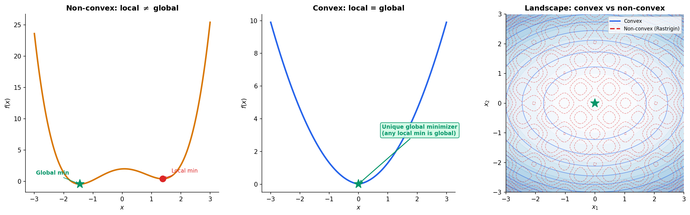
Here is the single most important fact in all of optimization:
Every local minimum of a convex function is a global minimum.
This one sentence is why convex optimization is tractable and general optimization is not. In a non-convex landscape — say a deep neural network loss surface — gradient descent can get trapped in local minima, saddle points, or flat regions, and we have no guarantee that the point we converge to is anywhere near optimal. But if the function we’re minimizing is convex, then any point where the gradient vanishes (or, more generally, where lies in the subdifferential) is a global minimizer. No restarts, no escaping saddle points, no hoping for the best.
This topic develops the mathematical infrastructure behind that fact. We start with the two geometric primitives — convex sets (closed under line segments) and convex functions (whose epigraph is a convex set) — and build up through three layers:
- Characterization: First-order and second-order conditions that connect convexity to gradients and Hessians.
- Closure: Operations that preserve convexity — the toolkit that lets us certify complex functions as convex without checking from scratch.
- Duality: Conjugate functions and subdifferentials that extend calculus to non-smooth settings, enabling the analysis of functions like and that appear throughout modern ML.
The separating hyperplane theorem provides the geometric backbone: it says that disjoint convex sets can always be separated by a hyperplane. This seemingly simple geometric fact has far-reaching consequences — it is the foundation of support vector machines, LP duality, and the entire theory of Lagrangian optimization.
What We Cover
- Convex Sets — the line-segment definition, convex combinations, and a gallery of examples.
- Convex Hull & Extreme Points — how to construct the smallest convex set containing a given set.
- Convex Functions — the chord inequality, epigraphs, and Jensen’s inequality.
- First-Order & Second-Order Conditions — connecting convexity to tangent lines and Hessian eigenvalues (via the Spectral Theorem).
- Operations Preserving Convexity — nonneg. weighted sums, pointwise max, composition rules (DCP).
- Conjugate Functions — the Legendre–Fenchel transform and biconjugation.
- Subdifferentials & Subgradients — generalized gradients for non-smooth functions.
- Separation Theorems — the geometric foundation of duality.
- Computational Notes — DCP rules, CVXPY, and numerical convexity verification.
Convex Sets
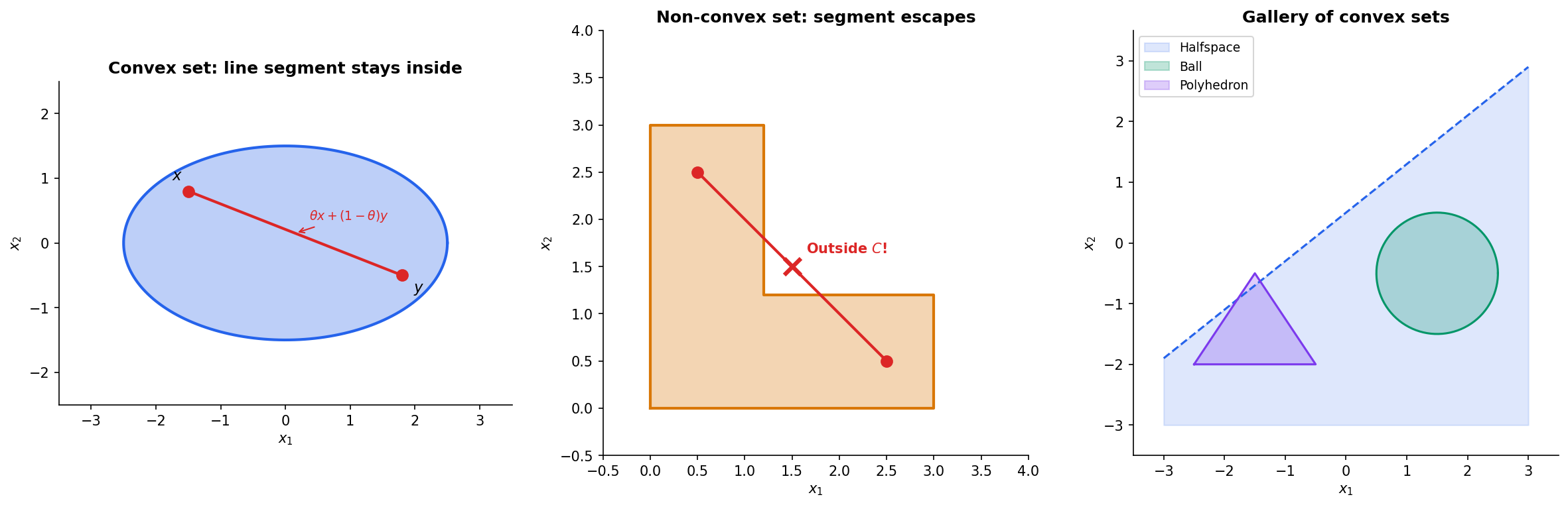
Everything begins with a definition that is geometric at its core: a set is convex if you can draw a straight line between any two of its points and the line stays inside the set.
Definition 1 (Convex Set).
A set is convex if for every and every :
Geometrically: the line segment from to lies entirely in .
This is the line-segment test, and it is the only thing you need to verify. An ellipse passes — every chord stays inside. An L-shape fails — there exist pairs of points whose connecting segment exits the set.
Definition 2 (Convex Combination).
A point is a convex combination of if where and . A set is convex if and only if it contains all convex combinations of its points.
A Gallery of Convex Sets
Convex sets are everywhere. Here are the workhorses:
- Halfspaces: for a fixed and . Every linear inequality defines a halfspace, and every halfspace is convex.
- Balls: in any norm. Euclidean balls, balls (cross-polytopes), balls (cubes).
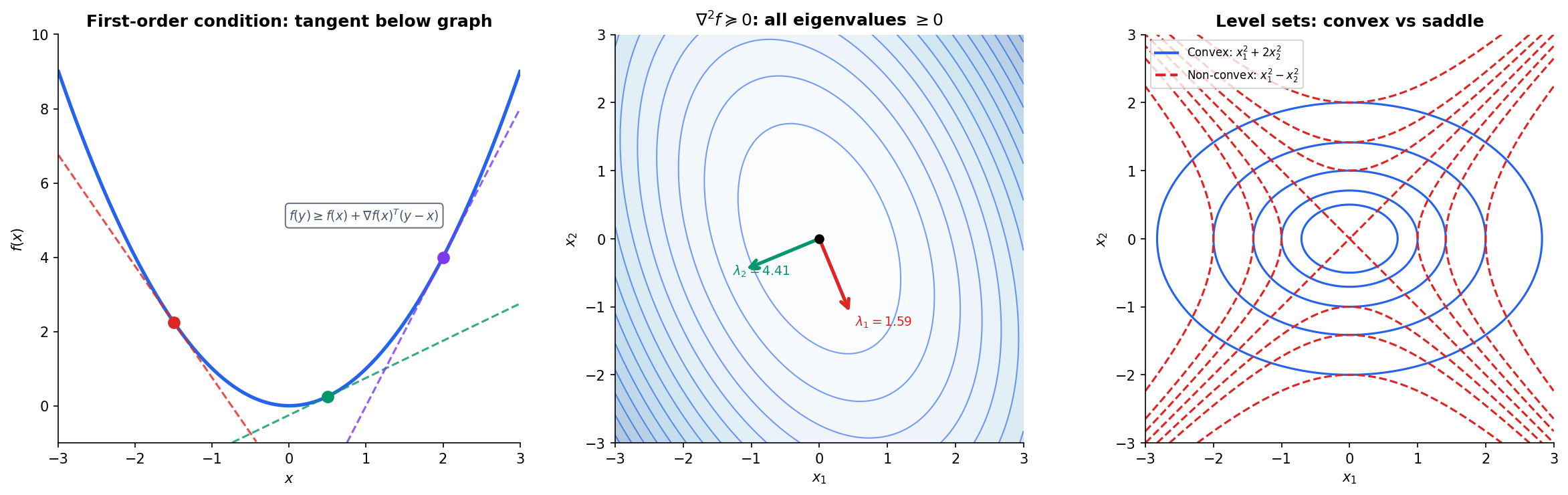
- Polyhedra: — intersections of finitely many halfspaces.
- Cones: (the second-order cone), and the positive semidefinite cone .
- The PSD cone : The set of all symmetric positive semidefinite matrices. Its structure is governed by the Spectral Theorem — a symmetric matrix is PSD if and only if all its eigenvalues are nonneg.
Convexity is preserved by intersection (any intersection of convex sets is convex), by affine maps (if is convex, then is convex), and by inverse affine maps (if is convex, then is convex).
Try the interactive explorer below — drag the two points around and watch whether the line segment between them stays inside the set.
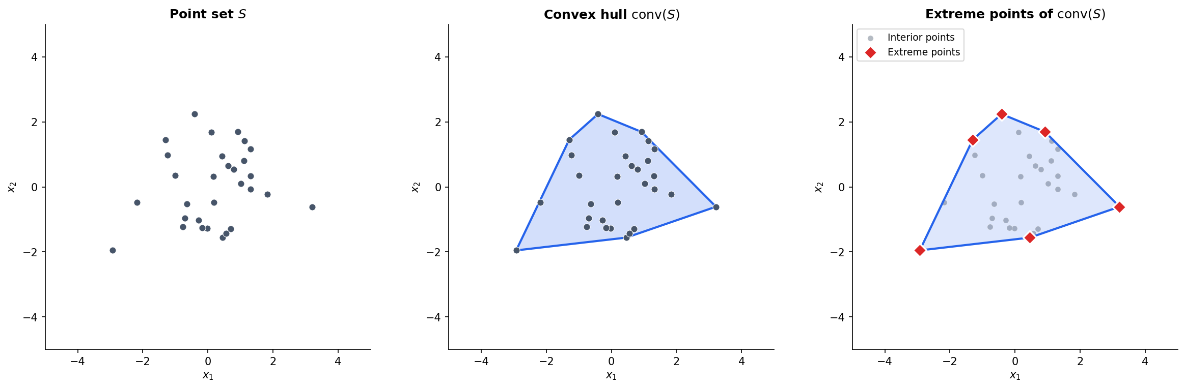
Convex Hull & Extreme Points
Given any set — convex or not — we can always construct the smallest convex set that contains it.
Definition 3 (Convex Hull).
The convex hull of a set , denoted , is the set of all convex combinations of points in :
Equivalently, is the intersection of all convex sets containing .
The vertices of the convex hull are special — they are the points that cannot be written as convex combinations of other points.
Definition 4 (Extreme Point).
A point is an extreme point of a convex set if there do not exist with and such that . In other words, is not a strict convex combination of two other points in .
The Krein–Milman theorem says that every compact convex set is the convex hull of its extreme points. This is a foundational result in functional analysis, and it has practical consequences: to optimize a linear function over a compact convex set, we need only check the extreme points — a fact that underpins the simplex method for linear programming.
# Compute and plot convex hull of a point set
import numpy as np
from scipy.spatial import ConvexHull

points = np.random.randn(30, 2) * 1.5
hull = ConvexHull(points)

# hull.vertices gives the indices of extreme points
extreme_points = points[hull.vertices]
Convex Functions
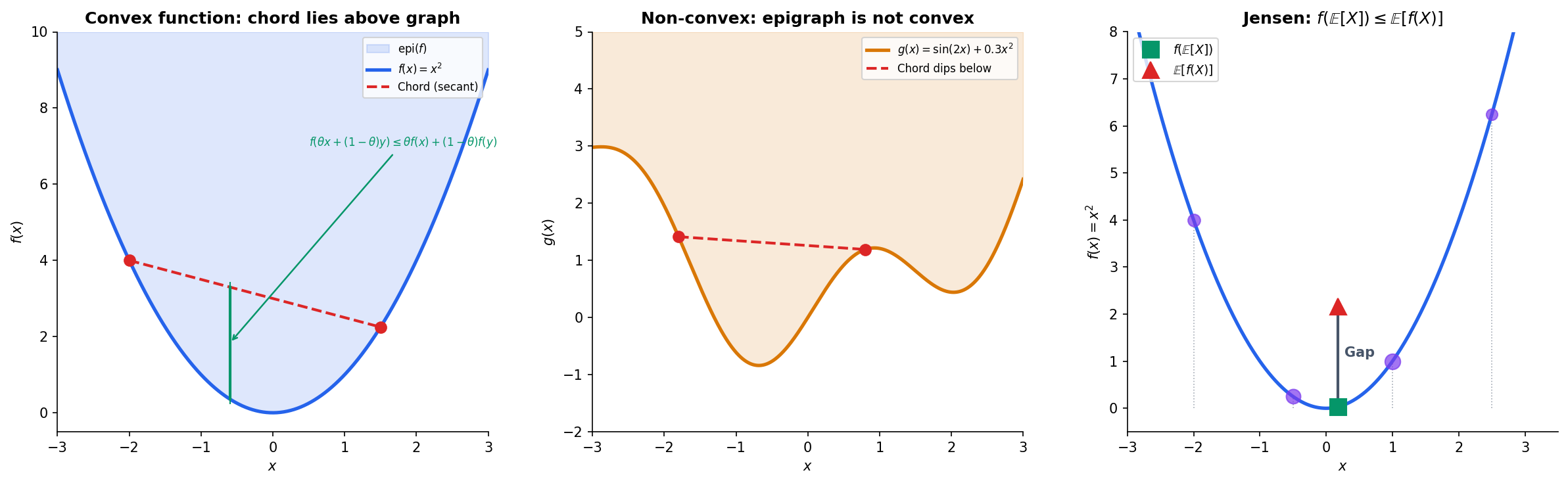
We now turn from sets to functions. The definition is again geometric: a function is convex if the chord between any two points on its graph lies above the graph.
Definition 5 (Convex Function).
A function is convex if for all in its domain and all :
The left side evaluates at the weighted average of and ; the right side is the weighted average of and . The inequality says: the function at the blend is at most the blend of the function values.
The connection between convex functions and convex sets runs through the epigraph.
Definition 6 (Epigraph).
The epigraph of a function is the set of points lying on or above its graph:
Proposition 1 (Epigraph Characterization of Convexity).
A function is convex if and only if is a convex set.
Proof.
() Suppose is convex. Take any two points , so and . For :
So , meaning is convex.
() Suppose is convex. For in the domain of , the points and lie in . Convexity of the epigraph gives:
which means , so is convex.
∎This equivalence is powerful: it lets us transfer results about convex sets directly to convex functions.
Jensen’s Inequality
The chord inequality generalizes from two points to any weighted average — this is Jensen’s inequality, one of the most widely used results in probability and information theory.
Theorem 1 (Jensen's Inequality).
If is convex and is a random variable with in the domain of , then:
Applying a convex function then averaging gives at least as much as averaging then applying the function.
Proof.
We prove the finite case. Let be values with weights summing to . We proceed by induction on .
Base case (): This is exactly the definition of convexity.
Inductive step: Assume the result holds for points. Write:
The inner sum is a convex combination of points (the weights sum to ). Call it . By convexity of :
By the inductive hypothesis, . Substituting:
∎
First-Order & Second-Order Conditions
The chord inequality is the definition, but there are more practical characterizations for differentiable functions.
The Tangent Line Condition
Theorem 2 (First-Order Condition for Convexity).
Suppose is differentiable on an open convex set. Then is convex if and only if for all :
The tangent hyperplane at any point is a global underestimator — the function never dips below its linearization.
Proof.
() Suppose is convex. For any :
Rearranging:
Taking , the right side becomes .
() Suppose the tangent inequality holds. For any and , let . Apply the tangent inequality at :
Multiply the first by , the second by , and add:
since .
∎The Hessian Condition
For twice-differentiable functions, convexity is equivalent to the Hessian being positive semidefinite — and this is where the Spectral Theorem enters.
Theorem 3 (Second-Order Condition for Convexity).
Suppose is twice differentiable on an open convex set. Then is convex if and only if the Hessian is positive semidefinite everywhere:
By the Spectral Theorem, the Hessian (a symmetric matrix) admits an eigendecomposition , and if and only if all eigenvalues .
This is the bridge between convexity and spectral theory. When we check whether a neural network loss function is locally convex around a critical point, we compute the Hessian and check its eigenvalues. The Spectral Theorem guarantees these eigenvalues are real and the eigenvectors are orthogonal — the entire machinery of eigendecomposition is built for exactly this purpose.
Example. Consider . The Hessian is:
Its eigenvalues are and — both positive. So is strictly convex.
Operations Preserving Convexity
Checking convexity from the definition or from the Hessian can be tedious. A more practical approach is to build convex functions from known convex building blocks using operations that preserve convexity. This is the idea behind Disciplined Convex Programming (DCP).
Nonnegative Weighted Sums
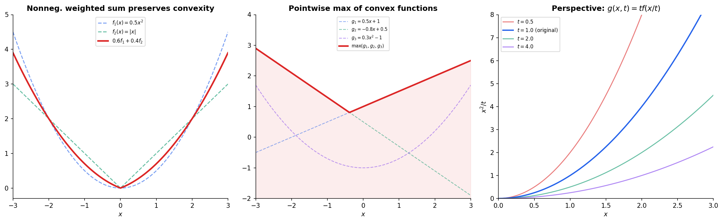
If are convex and , then is convex. This follows directly from the definition — the chord inequality distributes over sums.
Pointwise Maximum and Supremum
Proposition 2 (Pointwise Supremum Preserves Convexity).
If is a family of convex functions, then is convex.
Proof.
For any and :
Since and similarly for the second term:
∎
This result is remarkably useful. The maximum of finitely many convex functions is convex: is convex if each is. The norm is convex because it’s the max of convex functions .
Composition Rules (DCP)
The composition is convex under specific monotonicity conditions:
| Outer | Inner | Result | Condition |
|---|---|---|---|
| Convex, nondecreasing | Convex | Convex | — |
| Convex, nonincreasing | Concave | Convex | — |
| Concave, nondecreasing | Concave | Concave | — |
| Convex | Affine | Convex | Always |
These rules are the backbone of solvers like CVXPY. They verify convexity by parsing the composition structure of the objective function rather than computing second derivatives.
The Perspective Function
If is convex, then its perspective for is also convex. This construction appears in information theory (the KL divergence is the perspective of ) and in conic optimization.
Conjugate Functions
The Legendre–Fenchel conjugate provides a dual representation of convex functions — a powerful tool that transforms optimization problems into their dual forms.
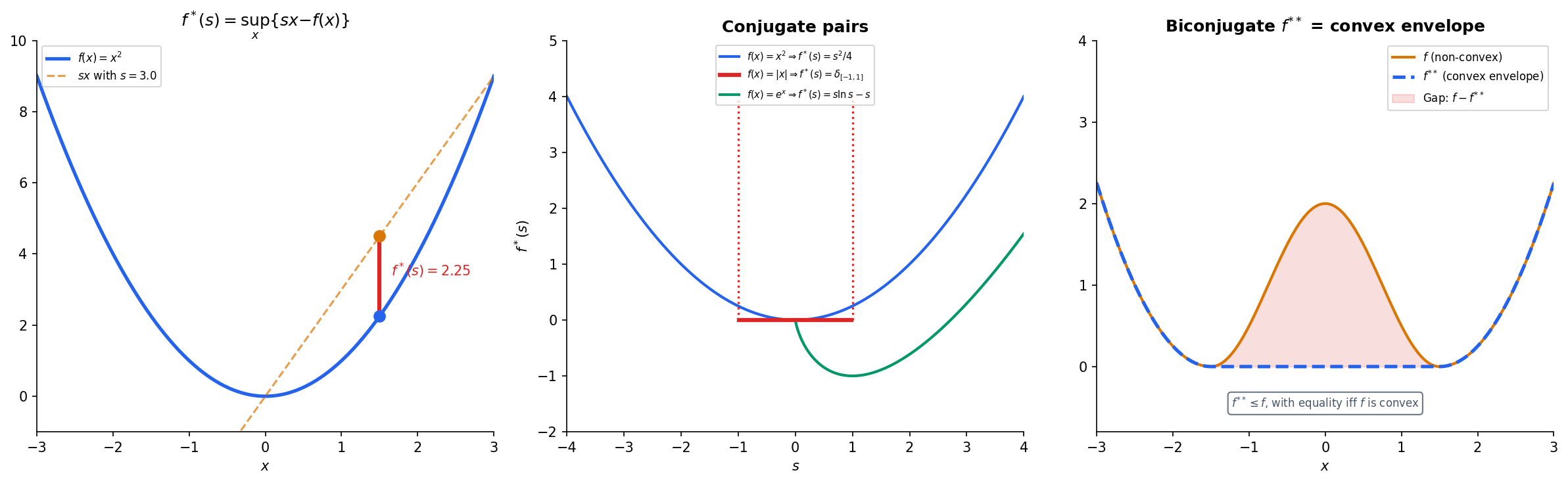
Definition 7 (Legendre–Fenchel Conjugate).
The conjugate (or Fenchel conjugate) of a function is:
For each slope , the conjugate measures the maximum gap between the linear function and .
The conjugate is always convex (it’s a pointwise supremum of affine functions in ), even if is not. Here are the classic conjugate pairs:
| Function | Conjugate |
|---|---|
| (any norm) | (indicator of dual norm ball) |
| for | |
| (indicator of ) | (support function) |
The biconjugation theorem is the central duality result: applying the conjugate twice recovers the original function — but only if it was convex to begin with.
Theorem 4 (Fenchel–Moreau Biconjugation).
If is a closed convex function (i.e., lower semicontinuous, convex, and proper), then .
If is not convex, then is the convex envelope of — the largest convex function that lies below .
Proof.
Proof sketch. We always have (apply the supremum definition twice). For the reverse inequality when is closed and convex: at any point , by the supporting hyperplane theorem, there exists such that . Then .
∎Biconjugation is the foundation of Lagrangian duality in optimization: the dual problem is the conjugate of the primal, and strong duality says that solving the dual recovers the primal optimum — under convexity.
Subdifferentials & Subgradients
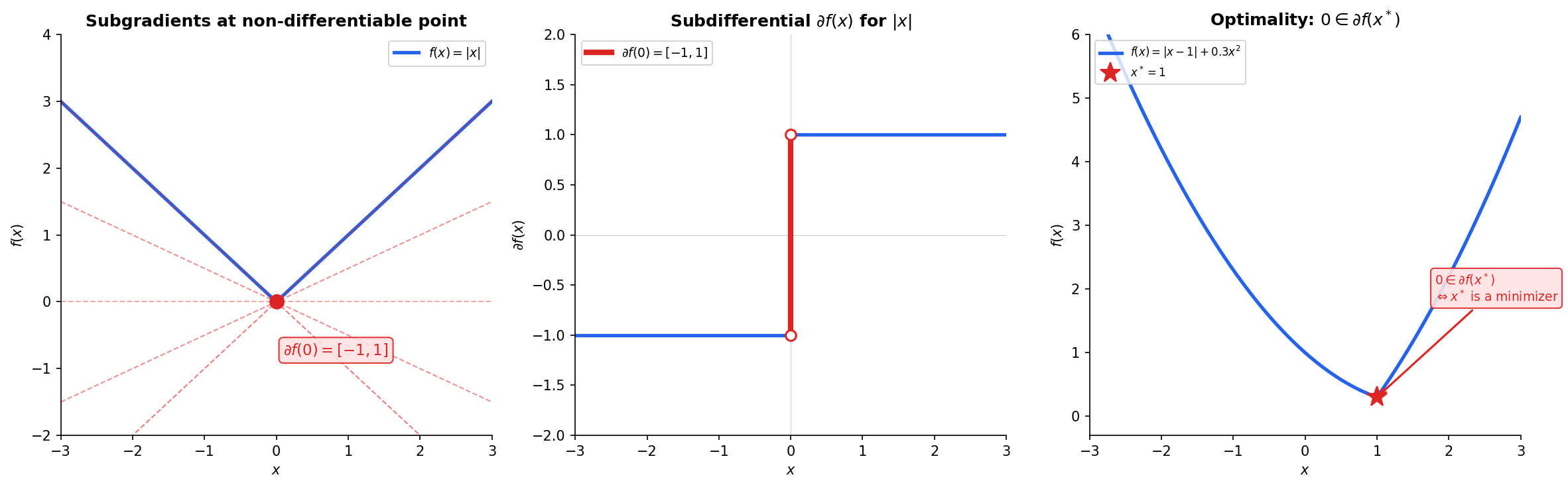
Not all convex functions are differentiable. The norm , the hinge loss , and the ReLU all have kinks where the gradient does not exist. Subgradients generalize the gradient to handle these cases.
Definition 8 (Subgradient).
A vector is a subgradient of a convex function at if:
That is, the affine function is a global underestimator of .
Definition 9 (Subdifferential).
The subdifferential of at is the set of all subgradients:
If is differentiable at , then — the subdifferential is a singleton containing the ordinary gradient. At a non-differentiable point, is a closed convex set of possible “slopes.”
Example: For :
- At : (the ordinary derivative)
- At :
- At : (any slope between and gives a valid underestimator)
The subdifferential gives us a complete optimality condition for convex optimization:
Theorem 5 (Subgradient Optimality Condition).
For a convex function , is a global minimizer if and only if:
Proof.
() If , then by the subgradient inequality with :
So is a global minimizer.
() If is a global minimizer, then for all . This means , so satisfies the subgradient inequality, i.e., .
∎Subdifferential Calculus
The subdifferential obeys sum and chain rules (with some caveats):
- Sum rule: (Minkowski sum). Equality holds when a constraint qualification is satisfied (e.g., one of the functions is continuous at ).
- Scalar multiplication: for .
- Chain rule: For with convex, .
- Connection to conjugates: if and only if if and only if (the Fenchel–Young equality).
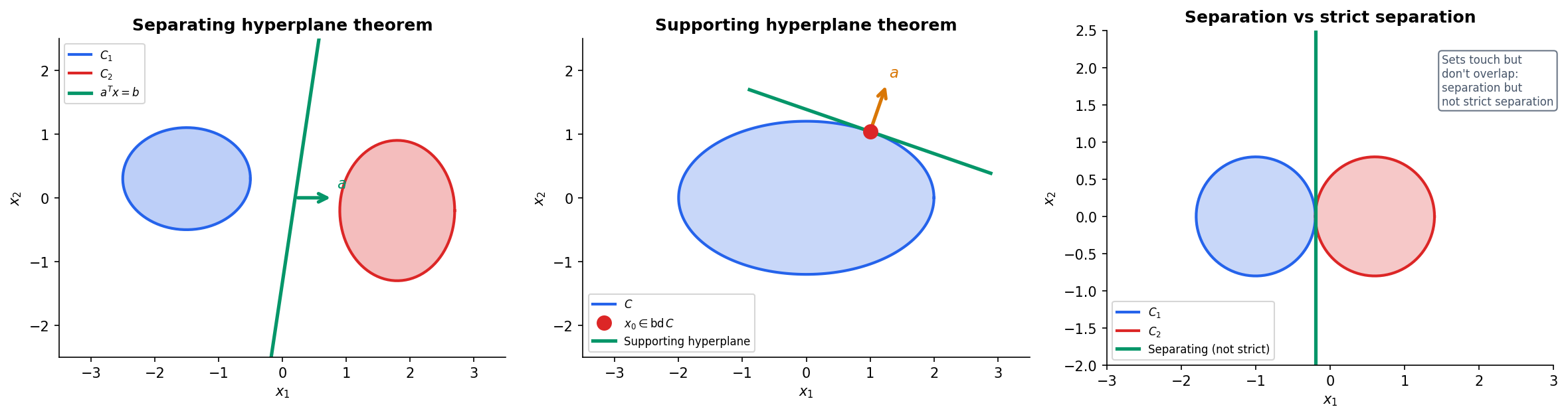
Separation Theorems
The separation theorems are the geometric bedrock of convex optimization. They say, loosely, that convex sets that don’t overlap can be separated by a hyperplane.
Theorem 6 (Separating Hyperplane Theorem).
Let and be nonempty, disjoint, convex sets in . Then there exists and such that:
The hyperplane separates and .
Proof.
Proof sketch. When and are closed and at least one is compact, we can find closest points and minimizing . The separating hyperplane passes through the midpoint with normal . The key step is showing that for any , the inner product (otherwise we could find a point in closer to , contradicting the minimality of ). The argument for is symmetric.
∎Theorem 7 (Supporting Hyperplane Theorem).
Let be a convex set and a boundary point. Then there exists a supporting hyperplane at : a hyperplane with and for all .
Geometrically: we can always find a hyperplane that is tangent to at any boundary point, with the entire set on one side.
These theorems have far-reaching consequences:
- SVM margin: The separating hyperplane between two classes of labeled data is the maximum-margin classifier.
- Farkas’ lemma: A direct consequence of separation, and the foundation of LP duality and the KKT conditions.
- Duality in convex optimization: The entire theory of Lagrangian duality rests on separating the epigraph of the objective from a set defined by the constraints.
Computational Notes
Disciplined Convex Programming (DCP)
Rather than checking convexity analytically, modern solvers like CVXPY use the DCP composition rules to verify convexity syntactically. A problem is DCP-compliant if the objective and constraints can be parsed into a composition tree where every node preserves convexity according to the rules in the table above.
import cvxpy as cp
import numpy as np

# Non-negative Lasso: min ||Ax - b||_2^2 + lambda * ||x||_1  s.t. x >= 0
A = np.random.randn(50, 20)
b = np.random.randn(50)
lam = 0.1

x = cp.Variable(20)
objective = cp.Minimize(cp.sum_squares(A @ x - b) + lam * cp.norm1(x))
constraints = [x >= 0]
problem = cp.Problem(objective, constraints)
problem.solve()

print(f"Optimal value: {problem.value:.4f}")
print(f"Solution sparsity: {np.sum(np.abs(x.value) < 1e-6)} / {x.size} zeros")
CVXPY verifies that sum_squares is convex nondecreasing, the affine map A @ x - b composes correctly, norm1 is convex, and x >= 0 is a valid convex constraint. If any rule is violated, CVXPY rejects the problem before solving.
Numerical Convexity Verification
For a function given as code rather than a formula, we can check convexity numerically by sampling the Hessian at random points and verifying :
# Check convexity by sampling Hessian eigenvalues
def check_convexity(f, grad2_f, n_samples=100, dim=5):
    """Returns True if all sampled Hessians are PSD."""
    for _ in range(n_samples):
        x = np.random.randn(dim)
        H = grad2_f(x)
        min_eig = np.linalg.eigvalsh(H)[0]
        if min_eig < -1e-10:
            return False
    return True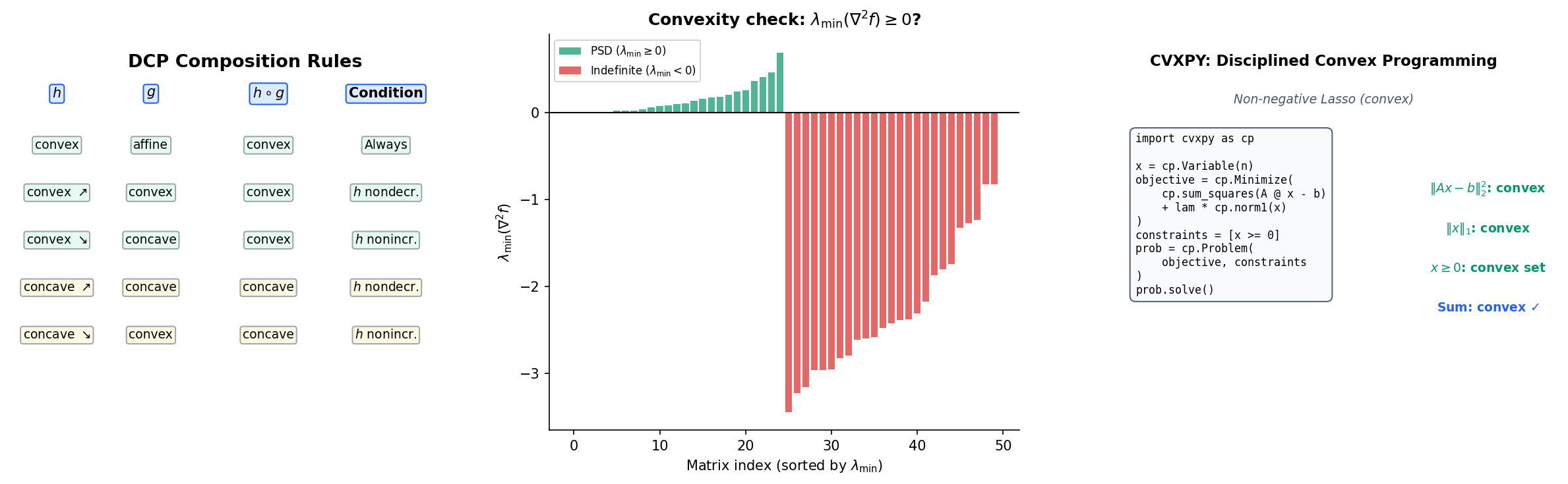
Connections & Further Reading
Convex analysis is the foundation of the Optimization track, connecting backward to spectral theory and forward to gradient methods, proximal operators, and duality theory.
| Topic | Connection |
|---|---|
| The Spectral Theorem | The second-order condition: (PSD Hessian) is verified through the eigendecomposition guaranteed by the Spectral Theorem. The PSD cone is a fundamental convex set. |
| Singular Value Decomposition | The nuclear norm is convex, and its subdifferential involves the SVD. Convex relaxations of rank constraints use the nuclear norm ball. |
| PCA & Low-Rank Approximation | PCA solves a non-convex rank-constrained problem. Its convex relaxation — nuclear norm minimization — is a cornerstone of compressed sensing and matrix completion. |
| Gradient Descent & Convergence | Convexity guarantees that gradient descent converges to the global minimum. The convergence rate depends on the strong convexity constant. |
| Proximal Methods | Subgradients motivate proximal operators — the proximal map of at minimizes , a regularized subgradient step. |
| Lagrangian Duality & KKT | Conjugate functions are the engine of Lagrangian duality. The separation theorems lead to Farkas’ lemma, which leads to the KKT conditions — the first-order optimality conditions for constrained convex optimization. |
| Quantile Regression | The pinball loss is piecewise-linear convex, and its empirical risk minimization is the canonical reduction of a piecewise-linear convex objective to a linear program — via the standard slack-variable split with (the canonical convex-analysis device). |
The Optimization Track
Convex Analysis is the root of the track: everything that follows either applies its results (gradient descent, proximal methods) or extends its duality machinery (Lagrangian duality, KKT conditions).
Convex Analysis (this topic)
    ├── Gradient Descent & Convergence
    │       └── Proximal Methods
    └── Lagrangian Duality & KKT
Connections
- The second-order convexity condition requires the Hessian to be positive semidefinite — the Spectral Theorem provides the eigendecomposition that lets us check this. PSD cones are fundamental convex sets whose structure is governed by the spectral theory of symmetric matrices. spectral-theorem
- The nuclear norm (sum of singular values) is a convex function, and its subdifferential involves the SVD. Low-rank matrix optimization problems rely on convex relaxations via the nuclear norm ball. svd
- PCA solves a non-convex rank-constrained problem whose convex relaxation (nuclear norm minimization) is a cornerstone of compressed sensing and matrix completion. pca-low-rank
- Tukey halfspace depth's axiomatic theorems and the convexity of depth contours (statistical-depth Proposition 1) live entirely in the language of supporting hyperplanes, halfspaces, and convex hulls. The convex-analysis toolkit is the natural setting for derivations of the Tukey median's geometric properties. statistical-depth
References & Further Reading
- book Convex Optimization — Boyd & Vandenberghe (2004) Chapters 2-3: Convex sets and convex functions — the primary reference for this topic
- book Convex Analysis — Rockafellar (1970) The foundational monograph — conjugate functions, subdifferentials, separation theorems
- book Introductory Lectures on Convex Optimization — Nesterov (2004) Chapter 2: Smooth convex optimization and first/second-order conditions
- book Convex Analysis and Minimization Algorithms I — Hiriart-Urruty & Lemaréchal (1993) Subdifferential calculus, conjugate duality, and Moreau envelopes
- paper Disciplined Convex Programming — Grant, Boyd & Ye (2006) DCP composition rules that underpin CVXPY and CVX
- paper Proximal Algorithms — Parikh & Boyd (2014) Section 2: Convex analysis background — subdifferentials, conjugates, Moreau envelopes