Statistical Depth

Overview

Statistical depth assigns each point in $\mathbb{R}^d$ a centrality score with respect to an empirical or population distribution, generalizing the median, quantile, and rank to dimensions where ordering is no longer well defined. The Tukey halfspace depth — the canonical construction — measures how surrounded a point is by the data: it is the smallest fraction of the sample on either side of any hyperplane through that point. Depth functions package multivariate location, spread, and outlyingness into a single object that obeys a clean axiomatic specification (Zuo and Serfling 2000), supports robust median estimation with breakdown $\ge 1/(d+1)$ (Donoho and Gasko 1992), and underwrites a small zoo of multivariate ML tools — the DD-classifier, depth-based outlier detection, and functional depth for curves and time series.

The topic structure: motivation and the Zuo–Serfling axioms (§1), Tukey halfspace depth as the canonical depth function (§2), a comparative survey of Mahalanobis, simplicial, projection, and spatial depths (§3), the asymptotic theory and computational complexity of Tukey depth (§4), ML applications via DD-classification, outlier detection, and functional depth (§5), and connections plus honest limits (§6).

The reader is assumed to be comfortable with measure-theoretic probability, weak convergence, and the basic vocabulary of convex geometry — halfspaces, supporting hyperplanes, convex hulls, simplices. Empirical-process limit theorems make a cameo in §4 and are sketched rather than developed from scratch.

This topic closes the T4 Nonparametric & Distribution-Free track. Where the other six T4 topics — Conformal Prediction, Quantile Regression, Rank Tests, Prediction Intervals, Extreme Value Theory, and the univariate machinery they share — operate one variable at a time, statistical depth is what those topics look like in $\mathbb{R}^d$ when there is no canonical order on the sample space.

1. From quantile to depth

In one dimension a sample has an unambiguous middle. The median of $X_1, \dots, X_n \in \mathbb{R}$ minimizes $\sum_i |X_i - \theta|$, splits the sample into halves, and is the level-$1/2$ value of the empirical quantile function $\hat F^{-1}(p) = \inf\{x : \hat F(x) \ge p\}$. The empirical CDF $\hat F$ orders the sample, the quantile function inverts that order, and rank-based machinery — Wilcoxon tests, sign tests, prediction intervals built from order statistics — drops out. All of it rests on the fact that $\mathbb{R}$ is totally ordered.

In $\mathbb{R}^d$ for $d \ge 2$ that order is gone. There is no canonical way to say which of two points $\mathbf{x}, \mathbf{y} \in \mathbb{R}^2$ comes “before” the other; the natural componentwise partial order leaves most pairs incomparable, and the obvious workarounds — the componentwise median, the Mahalanobis-distance “center,” the geometric median — each capture some aspect of multivariate centrality but disagree on most samples and behave badly under affine reparametrization. The question “which point in this 2D cloud is most central?” has several reasonable answers, and which one is correct depends on what we want centrality to do.

A depth function is the answer that asks what we want first and derives the construction second. It assigns each point $\mathbf{x} \in \mathbb{R}^d$ a real number — the depth of $\mathbf{x}$ with respect to a distribution $F$ — large when $\mathbf{x}$ sits in the bulk of $F$ and small when $\mathbf{x}$ is near the edge or far outside. The depth function is then a multivariate centrality score, and the deepest point is the multivariate median.

1.1 Why componentwise quantiles fail

The fastest way to feel the gap is to try the obvious fix. Given a 2D sample, take the median of the first coordinate and the median of the second coordinate; call the resulting point the componentwise median. The construction is fast, well-defined, and almost always wrong for what we mean by “the center of the cloud.”

Two failures appear immediately. The first is affine non-equivariance: rotate the sample by $45^\circ$ and the componentwise median moves as a function of the rotation, not as the rotated original median. The “center” depends on the choice of axes, which is exactly what we do not want for a notion that ought to track the geometry of the cloud rather than the bookkeeping of its representation. The second is lack of fit to non-axis-aligned bulk: when the sample concentrates along a tilted ellipse, the componentwise median can lie outside the bulk entirely, because the marginal medians know nothing about the off-diagonal correlation. The geometric median (Fréchet 1948) — the minimizer of $\sum_i \|\mathbf{x} - \mathbf{X}_i\|$ — fixes affine equivariance on rigid motions but still depends on the choice of norm and is not equivariant under arbitrary affine maps.

The mean and the Mahalanobis center handle affine equivariance correctly but inherit moment assumptions: the mean fails outright on heavy-tailed data, and the Mahalanobis center is anchored to the sample covariance, which has breakdown point $0$ — a single far outlier can drag the “center” anywhere we like.

What we want from multivariate centrality is a single function that (i) does not care about the choice of axes, (ii) puts the maximum at something that looks geometrically central regardless of the parametric family, (iii) decreases monotonically as we move away from that maximum, and (iv) does not let one or two outliers redefine where the bulk is. Listing those four desiderata is the Zuo–Serfling axiomatization.

1.2 What we want from a depth function

We pause to fix notation. Throughout this topic, $F$ denotes a probability distribution on $\mathbb{R}^d$, $\mathbf{X} \sim F$ a random vector with that distribution, and $\mathbf{X}_1, \dots, \mathbf{X}_n$ an iid sample from $F$ with empirical distribution $F_n = \frac{1}{n}\sum_{i=1}^n \delta_{\mathbf{X}_i}$. Affine transformations $\mathbf{x} \mapsto A\mathbf{x} + \mathbf{b}$ for nonsingular $A \in \mathbb{R}^{d \times d}$ and $\mathbf{b} \in \mathbb{R}^d$ are denoted $\mathcal{A}_{A,\mathbf{b}}$; the pushforward of $F$ under $\mathcal{A}_{A,\mathbf{b}}$ is written $F^{A,\mathbf{b}}$, the distribution of $A\mathbf{X} + \mathbf{b}$.

A depth function is a map $D : \mathbb{R}^d \times \mathcal{P}(\mathbb{R}^d) \to [0, \infty)$, written $D(\mathbf{x}; F)$, that takes a point and a distribution and returns a non-negative real number. The reading is: $D(\mathbf{x}; F)$ measures how central $\mathbf{x}$ is with respect to $F$, with larger values meaning more central. Several depth functions in §3 take values in $[0, 1]$; the unit-interval normalization is conventional but not part of the definition.

The deepest point of $F$ is any maximizer

$\boldsymbol{\mu}_D(F) \;\in\; \arg\max_{\mathbf{x} \in \mathbb{R}^d} D(\mathbf{x}; F).$

For most depth functions $\boldsymbol{\mu}_D$ is uniquely determined when $F$ has a density, but it is generally a set when $F$ is empirical — we will see in §2 that the empirical Tukey median is a region, not a point, and a tie-breaking rule (typically the centroid of that region) returns a single estimate.

The depth contour at level $\alpha \ge 0$ is the upper level set

$D_\alpha(F) \;=\; \{\mathbf{x} \in \mathbb{R}^d : D(\mathbf{x}; F) \ge \alpha\}.$

For halfspace depth these contours are nested closed convex sets indexed by $\alpha \in [0, 1/2]$; they form the multivariate analogue of confidence regions or quantile curves.

1.3 The Zuo–Serfling axioms

Zuo and Serfling (2000) formalize what a depth function ought to do via four axioms that together pick out a flexible but well-disciplined class. We state the axioms first, then motivate each one against the failure modes of §1.1.

The motivation for each axiom matches one of §1.1’s pain points. (D1) removes the dependence on the choice of axes. (D2) anchors the depth function to a geometric notion of “center” whenever one exists unambiguously. (D3) says depth respects the geometry of “moving outward.” (D4) rules out the pathology where a depth function fails to distinguish “very far away” from “merely far away” — a regularity condition mostly used to guarantee that maxima exist.

The axioms are not independent — (D2) and (D3) interact through the choice of “center” — and in the literature several authors propose weaker variants. For this topic we adopt Zuo and Serfling’s original four. Each depth function in §3 will be checked against the axioms; one of them, Mahalanobis depth, will fail (D1) in spirit on non-elliptical distributions, and the failure is exactly visible in the side-by-side panel.

1.4 Running examples

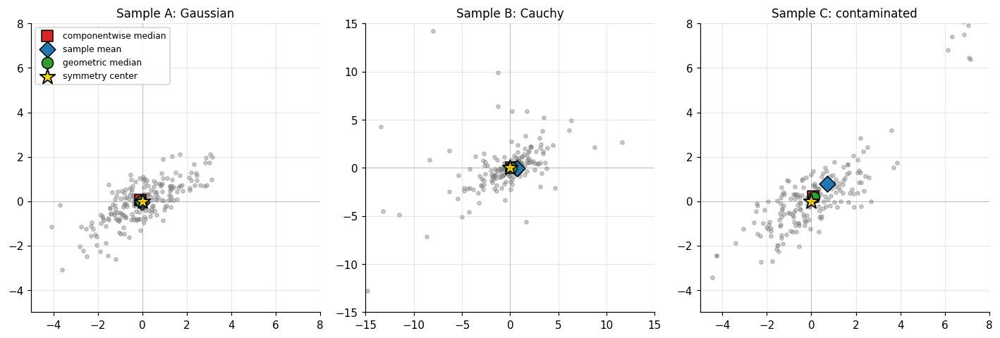
Three samples thread §§1–6.

Sample A — bivariate Gaussian. $\mathbf{X}_1, \dots, \mathbf{X}_n \stackrel{\text{iid}}{\sim} \mathcal{N}(\mathbf{0}, \boldsymbol{\Sigma})$ with

$\boldsymbol{\Sigma} = \begin{pmatrix} 2 & 1 \\ 1 & 1 \end{pmatrix}, \qquad n = 200.$

This is the canonical exemplar: an elliptical distribution where every depth function in §3 satisfies the axioms and contours are nested ellipses. The deepest point is the origin; depth contours are concentric tilted ellipses oriented along the leading eigenvector of $\boldsymbol{\Sigma}$.

Sample B — bivariate Cauchy. Same scale matrix as Sample A. The Cauchy has no mean and no covariance, so the sample mean and Mahalanobis center are unstable — but Tukey, simplicial, and projection depth still produce well-behaved contours, and the deepest point is still the origin (now interpreted as the symmetry center rather than the mean).

Sample C — contaminated Gaussian. A mixture, $0.90\, \mathcal{N}(\mathbf{0}, \boldsymbol{\Sigma}) + 0.10\, \mathcal{N}(\boldsymbol{\mu}_{\text{out}}, \mathbf{I})$ with $\boldsymbol{\mu}_{\text{out}} = (8, 8)^\top$. Depth functions with high breakdown (Tukey, simplicial, projection) keep the deepest point near $\mathbf{0}$ regardless of contamination; depth functions anchored to moments (Mahalanobis on the empirical covariance) drift toward the contamination cluster.

The figure below shows all three samples side by side together with three reasonable-looking but disagreeing notions of “center”: the componentwise median, the sample mean, and the geometric median (the minimizer of $\sum_i \|\mathbf{x} - \mathbf{X}_i\|$ via Weiszfeld’s iteration). On the Gaussian they roughly agree; on the Cauchy the mean is unstable; on the contaminated sample they disagree by a meaningful amount and none of them is obviously right. The §2 Tukey median, by contrast, will sit near the origin in all three panels.

2. Tukey halfspace depth

Tukey (1975) proposed the construction that defines the canonical multivariate centrality score. The idea is geometric: for a point $\mathbf{x}$ to be deep, every line through $\mathbf{x}$ should split the sample roughly in half; a point near the boundary of the cloud, by contrast, has at least one line through it that puts almost all of the sample on one side. The minimum count over all such lines — equivalently, all halfspaces with $\mathbf{x}$ on their boundary — is the halfspace depth.

2.1 Definition

Recall a closed halfspace in $\mathbb{R}^d$ is a set of the form

$H_{\mathbf{u}, c} \;=\; \{\mathbf{y} \in \mathbb{R}^d : \mathbf{u}^\top \mathbf{y} \ge c\}, \qquad \mathbf{u} \in \mathbb{S}^{d-1}, \; c \in \mathbb{R},$

where $\mathbb{S}^{d-1} = \{\mathbf{u} \in \mathbb{R}^d : \|\mathbf{u}\| = 1\}$ is the unit sphere. The boundary hyperplane is $\partial H_{\mathbf{u}, c} = \{\mathbf{y} : \mathbf{u}^\top \mathbf{y} = c\}$.

Equivalently, every closed halfspace containing $\mathbf{x}$ has the form $H_{\mathbf{u}, c}$ with $\mathbf{u}^\top \mathbf{x} \ge c$. The worst case (smallest $F$-mass) is achieved by halfspaces whose boundary passes exactly through $\mathbf{x}$, so the infimum reduces to

$\operatorname{HD}(\mathbf{x}; F) \;=\; \inf_{\mathbf{u} \in \mathbb{S}^{d-1}} F\bigl(\{\mathbf{y} : \mathbf{u}^\top(\mathbf{y} - \mathbf{x}) \ge 0\}\bigr) \;=\; \inf_{\mathbf{u} \in \mathbb{S}^{d-1}} \mathbb{P}\bigl(\mathbf{u}^\top(\mathbf{X} - \mathbf{x}) \ge 0\bigr).$

The reading is direct: pick any direction $\mathbf{u}$, slide a hyperplane through $\mathbf{x}$ orthogonal to $\mathbf{u}$, and count the $F$-probability on the $\mathbf{u}$-side. Halfspace depth is the worst (smallest) such fraction.

The unit-interval normalization is conventional: $\operatorname{HD}_n(\mathbf{x}) \in \{0/n, 1/n, \dots, n/n\}$. The maximum possible value is bounded by $1/2$ in $d \ge 2$ for any $F$ with no atom at $\mathbf{x}$ (one can always find a hyperplane through $\mathbf{x}$ that puts at most half the mass on either side), and the upper bound is achieved only at the halfspace median — defined in §2.4.

A worked example fixes ideas. Consider four points in $\mathbb{R}^2$ at the corners of a unit square, $\{(0,0), (1,0), (0,1), (1,1)\}$, and the query point $\mathbf{x} = (0.5, 0.5)$. Every line through $\mathbf{x}$ either passes through two opposite corners — in which case those corners lie on the boundary, included in the closed halfspace, and the closed halfspace contains all four points on one side — or strictly separates two corners from two corners. The minimum closed-halfspace count is $2$, so $\operatorname{HD}_n(\mathbf{x}) = 2/4 = 1/2$. By contrast, the corner $\mathbf{x}' = (0, 0)$ has $\operatorname{HD}_n(\mathbf{x}') = 1/4$ (only one of the four points lies in the halfspace $\{y_1 < 0\} \cup \{y_1 = 0, y_2 \ne 0\}$), and any point $\mathbf{x}'' = (2, 2)$ outside the square has $\operatorname{HD}_n(\mathbf{x}'') = 0$.

2.2 Verifying the Zuo–Serfling axioms

Halfspace depth was the prototype Zuo and Serfling had in mind when they wrote down the four axioms; verification is short and clean.

So Tukey halfspace depth is a Zuo–Serfling depth function — the construction satisfies the entire axiomatic specification. The proofs above used only the closed-halfspace formulation; the same argument works for the empirical version with $F_n$ in place of $F$.

2.3 The Tukey median and contour convexity

The Tukey median of $F$ is any maximizer of $\operatorname{HD}(\,\cdot\,; F)$:

$\boldsymbol{\mu}_T(F) \;\in\; \arg\max_{\mathbf{x} \in \mathbb{R}^d} \operatorname{HD}(\mathbf{x}; F).$

For populations $F$ with a density and central symmetry, the proof of (D2) shows $\boldsymbol{\mu}_T(F) = \boldsymbol{\mu}$ uniquely. For the empirical distribution $F_n$, the maximizer is generally a region, not a point: the level set $\{\mathbf{x} : \operatorname{HD}_n(\mathbf{x}) = \alpha^*\}$ at the maximum depth $\alpha^*$ is a non-empty closed convex set, and the conventional point estimator is its centroid.

The convexity comes from a structural fact about depth contours.

The depth contours are closed convex sets nested by depth level, and the Tukey median is the deepest such set. This convexity property is what makes halfspace depth particularly useful for constructing multivariate confidence regions.

2.4 Computing 2D Tukey depth

Computing $\operatorname{HD}_n(\mathbf{x})$ in $\mathbb{R}^d$ requires evaluating an infimum over the unit sphere $\mathbb{S}^{d-1}$. In 2D this infimum reduces to a search over the $n$ angular bearings of the data points relative to $\mathbf{x}$, and there is an exact $O(n \log n)$ algorithm — the rotating-halfplane sweep (Rousseeuw and Ruts 1996).

Algorithm (Rousseeuw–Ruts, sketch). Let $\mathbf{y}_i = \mathbf{X}_i - \mathbf{x}$. Compute angles $\theta_i = \arctan2(y_{i,2}, y_{i,1}) \in [-\pi, \pi)$ for each non-coincident $\mathbf{y}_i$. Sort the angles. The closed halfplane through $\mathbf{x}$ with normal at angle $\alpha + \pi/2$ contains exactly the points whose angles fall in $[\alpha, \alpha + \pi]$. As $\alpha$ sweeps through $[0, 2\pi)$, the count changes only when $\alpha$ crosses one of the $\theta_i$ or one of the $\theta_i - \pi$ markers; the minimum over all sweep positions, plus the count of points coincident with $\mathbf{x}$ (which lie on every halfplane boundary), is the depth count. The whole computation is dominated by the sort, $O(n \log n)$.

The companion algorithm in $d \ge 3$ is more involved: exact computation reduces to enumerating all hyperplanes through the query point and $d-1$ data points, an $O(n^{d-1})$ operation. Aloupis (2006) shows that exact computation of the depth at a single point — without requiring the full enumeration — is NP-hard when $d$ is part of the input. We return to that result in §4.4.

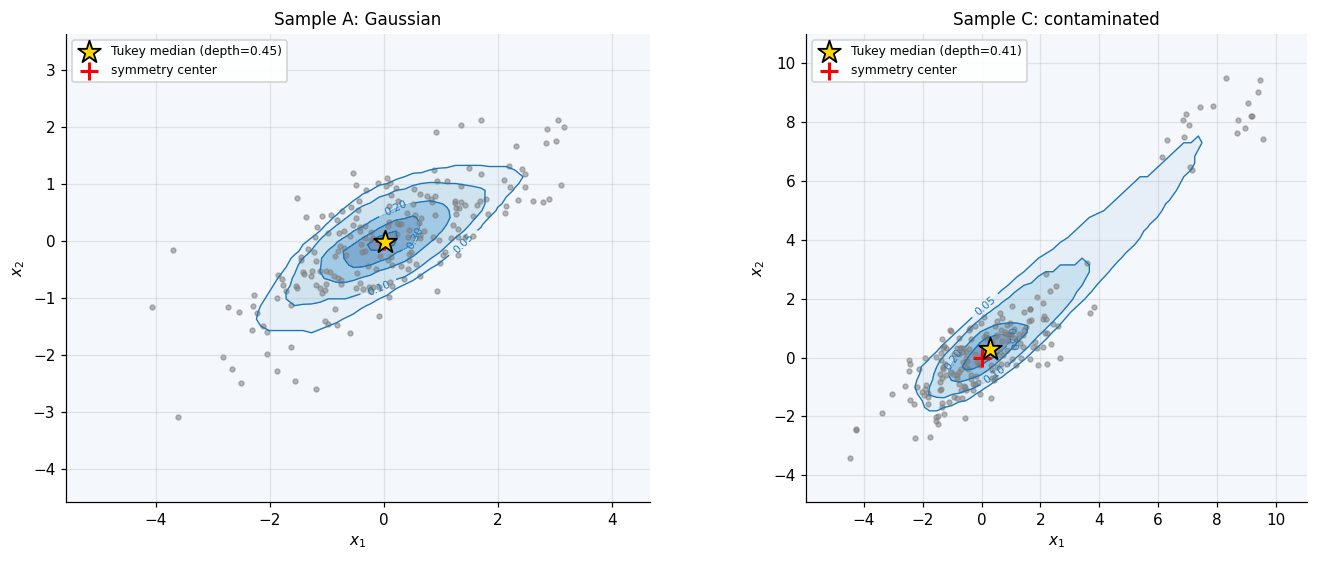
2.5 Depth contours

With the 2D algorithm in hand we can plot depth contours $\{\mathbf{x} : \operatorname{HD}_n(\mathbf{x}) \ge \alpha\}$ as a function of $\alpha$. For Sample A the contours are nested and roughly concentric ellipses, oriented along the leading eigenvector of $\boldsymbol{\Sigma}$, with the maximum depth attained near the origin at value $\approx 1/2$. For Sample C the contamination cluster does not redirect the contours: the deepest region remains near the origin, the outliers register only as a small bump on the outer (low-$\alpha$) contours. This is the visual demonstration that halfspace depth has high breakdown — a quantitative argument follows in §4.2.

The interactive widget below recomputes contours on the fly. Switch the sample selector to compare A, B, C; drag the pink crosshair to read live depth at any query point; raise the grid resolution for a sharper picture (at the cost of more depth queries per redraw).

Sample:A — GaussianB — CauchyC — contaminated

Grid:40×40

query (0.00, 0.00)HDₙ = 0.415

iid bivariate Gaussian; all four §1 centres agree near the origin.

★ marks the empirical Tukey median (centroid of the deepest grid cell). Drag the pink crosshair to read depth at any query point. Grid resolution trades accuracy against wait time — gridSize² Tukey-depth queries per redraw.

3. A zoo of depth functions

Tukey halfspace depth is canonical but not unique. Several other constructions satisfy the Zuo–Serfling axioms, each making different tradeoffs along three axes the §2 algorithm exposed: how fast the depth is to compute, how strongly the depth depends on parametric model assumptions, and how the depth scales with dimension. We catalogue four of the most useful — Mahalanobis, simplicial, projection, and spatial depth — verify the relevant axioms, and put the contours side by side on a common sample.

3.1 Mahalanobis depth

The fastest depth function — closed-form, requiring only a $d \times d$ matrix inverse — is the one anchored to the first two moments.

The empirical version uses the sample mean and sample covariance: $\operatorname{MD}_n(\mathbf{x}) = (1 + (\mathbf{x} - \bar{\mathbf{X}})^\top \mathbf{S}^{-1} (\mathbf{x} - \bar{\mathbf{X}}))^{-1}$.

Mahalanobis depth satisfies (D1)–(D4): the affine-invariance proof is one line, since under $\mathbf{x} \mapsto A\mathbf{x} + \mathbf{b}$ the mean shifts to $A\boldsymbol{\mu} + \mathbf{b}$, the covariance shifts to $A\boldsymbol{\Sigma} A^\top$, and the quadratic form $(\mathbf{x} - \boldsymbol{\mu})^\top \boldsymbol{\Sigma}^{-1}(\mathbf{x} - \boldsymbol{\mu})$ is preserved exactly. The maximum is attained at $\boldsymbol{\mu}_F$ with value $1$; monotonicity along rays is the convexity of quadratic forms; vanishing at infinity is automatic.

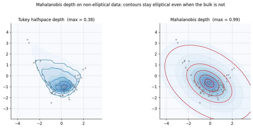
The catch is what maximum it produces. The $\arg\max$ of Mahalanobis depth is the mean, not the symmetry center. For a centrally symmetric $F$ with finite covariance the two coincide, so (D2) holds. For a non-elliptical $F$ — say, a banana-shaped distribution — Mahalanobis depth still produces ellipsoidal contours centered at the mean, even when the actual bulk of $F$ is far from elliptical. The depth is not wrong in the axiomatic sense; it is committed to the parametric ellipsoid, and any deviation from that model leaks straight into the depth contours. The breakdown is also the breakdown of the sample covariance: zero. A single far outlier moves $\mathbf{S}$ enough that $\mathbf{S}^{-1}$ tilts toward the outlier, and the deepest point drifts.

3.2 Simplicial depth

Liu (1988, 1990) proposed a depth function defined entirely in terms of the convex-hull geometry of random simplices.

The empirical version is a U-statistic of order $d+1$:

$\operatorname{SD}_n(\mathbf{x}) \;=\; \binom{n}{d+1}^{-1} \sum_{1 \le i_1 < \cdots < i_{d+1} \le n} \mathbb{1}\bigl\{\mathbf{x} \in \operatorname{conv}(\mathbf{X}_{i_1}, \dots, \mathbf{X}_{i_{d+1}})\bigr\}.$

The U-statistic structure is exactly what Liu’s result exploits: the kernel $h$ is symmetric, bounded, and has expectation $\operatorname{SD}(\mathbf{x}; F)$. Standard U-statistic theory (Hoeffding 1948) gives consistency, asymptotic normality, and explicit variance formulas for $\operatorname{SD}_n(\mathbf{x})$.

Simplicial depth is fully nonparametric (no moment assumptions), affine invariant, and satisfies a clean U-statistic-based asymptotic theory. Its computational cost, however, is severe in high dimensions: the U-statistic of order $d+1$ has $\binom{n}{d+1}$ terms, and even in 2D this is $\binom{n}{3} \asymp n^3/6$ point-in-triangle tests per query.

3.3 Projection depth

Random projections give a depth function that scales gracefully with dimension at the cost of trading exactness for a Monte-Carlo approximation.

The reading: project $F$ onto direction $\mathbf{u}$ to get the univariate distribution of $\mathbf{u}^\top \mathbf{X}$. Compute the standardized univariate distance from $\mathbf{u}^\top \mathbf{x}$ to the projected median. Take the supremum over directions. The deepest point in $\mathbb{R}^d$ is the one whose projected position is closest to the projected median in every direction — the multivariate generalization of “the median of every projection.”

In practice, the supremum over $\mathbb{S}^{d-1}$ is approximated by sampling $K$ random unit directions and taking the maximum:

$\widehat{\operatorname{PD}}_K(\mathbf{x}) \;=\; \frac{1}{1 + \max_{k=1,\dots,K} \frac{|\mathbf{u}_k^\top \mathbf{x} - m_k|}{\operatorname{MAD}_k}}.$

The cost is $O(K \cdot n)$ per query — linear in dimension and trivially parallel. Projection depth satisfies (D1)–(D4): affine invariance follows because the median and MAD are univariate-affine equivariant, and the supremum over $\mathbb{S}^{d-1}$ pulls back the same way Tukey’s does. The approximation $\widehat{\operatorname{PD}}_K \to \operatorname{PD}$ holds at every fixed $\mathbf{x}$ by the strong law applied to the supremum over a uniform sample on the sphere; the error is $O_p(\sqrt{\log K / K})$ uniformly on a compact set.

3.4 Spatial depth

Spatial depth (Vardi and Zhang 2000; Serfling 2002) replaces the sup-over-directions structure of projection depth with an $L^1$ optimality criterion.

The empirical version uses the sample mean of the unit-direction vectors. The geometric reading is clean. Each $\mathbf{X}_i$ contributes a unit vector pointing from $\mathbf{x}$ toward $\mathbf{X}_i$. If $\mathbf{x}$ sits at the geometric median of the sample, the unit vectors balance: their average is close to $\mathbf{0}$, so $\operatorname{Sp}_n(\mathbf{x}) \approx 1$. If $\mathbf{x}$ sits on the periphery, all the unit vectors point roughly the same way, the average has large norm, and $\operatorname{Sp}_n(\mathbf{x}) \approx 0$. The deepest point is the spatial median, which coincides with the Fréchet geometric median.

Spatial depth is affine equivariant only under orthogonal transformations — it depends on the choice of norm via the unit-direction normalization. For elliptically distributed data, this matters less than one might expect, because all relevant comparisons are in $L^2$. The cost is $O(n)$ per query, the cheapest of the four after Mahalanobis.

3.5 Side-by-side comparison

All four depth functions evaluated on Sample A produce qualitatively similar contour pictures — nested, roughly elliptical, peaked near the origin. The differences appear in (a) the rate at which contours decay outward, (b) sensitivity to contamination, and (c) whether the contour shape can deviate from an ellipse when the underlying distribution does. The five-panel figure below shows the contours on a common Gaussian sample.

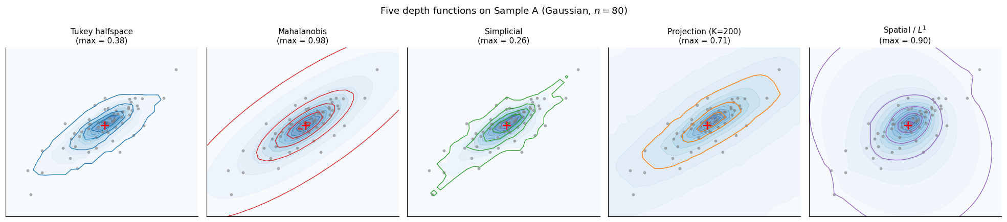
The interesting failure mode appears on non-elliptical data, where Mahalanobis depth’s commitment to the ellipsoid model leaks into the contours and produces depth structure that does not track the actual density of the sample.

The interactive comparison below lets you switch the sample (Gaussian / banana) and the right-hand depth function. The left panel always shows Tukey halfspace as the affine-invariant canonical reference. The simplicial branch is capped at $n = 60$; for $K$-direction projection depth, the inline approximation runs at $K = 200$.

Sample:GaussianBanana

Compare to:MahalanobisProjection (K=200)Spatial / L¹Simplicial (slow at n=60)

Gaussian (Σ tilted) · n = 60

On Gaussian data all five depths produce nearly affine images of one another — the elliptical bulk doesn't punish any choice. On the banana sample, Mahalanobis depth's elliptical commitment shows: contours stay aligned with the sample covariance even though the bulk bends. Tukey halfspace depth tracks the bend; the others vary.

4. Theory and computation

The §§2–3 implementations would be of limited value without theoretical guarantees that the empirical depth converges to its population counterpart, that the Tukey median is robust in a quantifiable sense, and that the asymptotic behaviour of empirical depth has a known limit law. This section assembles those guarantees and pairs each with its computational counterpart.

4.1 Consistency

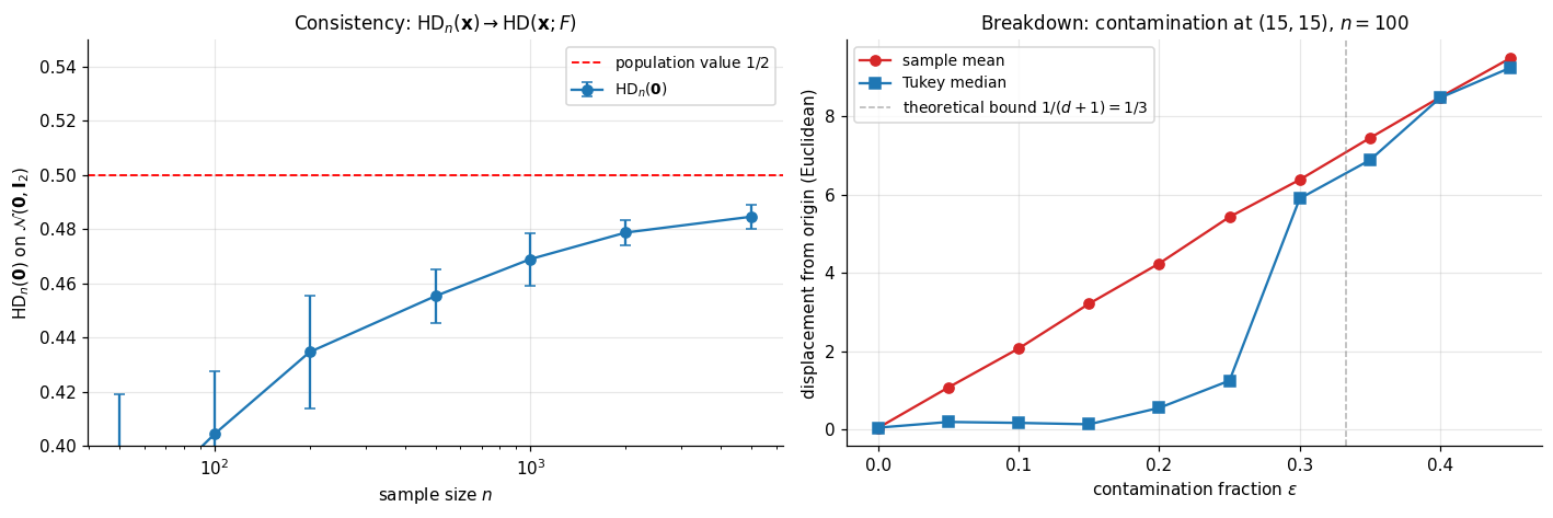
Halfspace depth at a fixed point is consistent under minimal assumptions on $F$.

The same argument gives consistency for projection depth (with the additional assumption that the population MAD is bounded away from $0$), spatial depth (with no atom at $\mathbf{x}$), and Mahalanobis depth (under the additional finite-second-moment condition the definition requires).

4.2 Breakdown of the Tukey median

The Tukey median’s breakdown point — the smallest fraction of contamination that can move it arbitrarily far — gives a quantitative version of the §2.5 contour-stability picture.

In $d = 2$ the bound gives $\varepsilon^* \ge 1/3$, comfortably above the $1/n$ breakdown of the sample mean.

4.3 Asymptotic distribution

Pointwise convergence (Theorem 3) is the consistency baseline. The next question is the rate.

The unique-minimizer assumption is essential: at points where the depth-defining infimum is attained at a set of directions (e.g., a centrally symmetric distribution at its center, where every direction attains $1/2$), the Hadamard-differentiability argument fails and the limit distribution becomes the supremum of a Gaussian process over the optimal-direction set.

4.4 Computational complexity

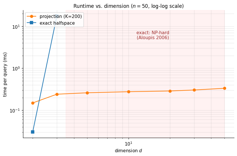
The §2 sweep gave $O(n \log n)$ for one query in 2D. The general-$d$ exact algorithm scales much worse.

The result is stated and not proved here — the proof is a reduction from the maximum-bisection problem and requires a separate combinatorial-geometry treatment. The practical consequence is decisive: exact computation of halfspace depth is restricted to fixed low dimension. The $O(n^{d-1})$ exact algorithm via hyperplane enumeration is feasible for $d \le 3$ (where it is $O(n^2)$) and only marginally feasible for $d = 4$ at moderate $n$. For $d \ge 5$ the practitioner must fall back on the random-direction approximation $\widehat{\operatorname{HD}}_K(\mathbf{x}) = \min_{k=1,\dots,K} F_n(H_{\mathbf{u}_k, \mathbf{u}_k^\top \mathbf{x}})$.

4.5 Projection-depth approximation efficacy

How accurate is the random-direction approximation as a function of $K$? The §3.3 analysis gave $\widehat{\operatorname{PD}}_K \to \operatorname{PD}$ with error $O_p(\sqrt{\log K / K})$. The same bound applies to the random-direction approximation of halfspace depth itself, since both are infimum-over-the-sphere objects. In practice $K = 200$ is sufficient for sub-percent error on moderately concentrated samples.

The widget below re-runs the benchmark live. Slide $K$ to see the projection-depth time scale linearly in directions; slide $n$ to see both methods scale at their predicted rates.

K (directions):200

n (sample):50

Per-query timing in milliseconds. Exact halfspace runs only at d ∈ {2, 3} per the §4.4 NP-hardness result.

Projection depth's roughly flat curve in d (cost is O(K · n), independent of dimension after the projection step) is the punchline of §4.5: in practice, the only depth that scales is the approximate one. Increasing K trades accuracy for cost — the random-direction approximation has Op(√(log K / K)) error.

5. ML applications

The depth machinery of §§2–4 was developed without reference to a specific ML problem, but it slots cleanly into three: nonparametric classification through the DD-plot, multivariate outlier detection that does not assume ellipticity, and analysis of functional data — random samples in which each observation is a curve rather than a vector.

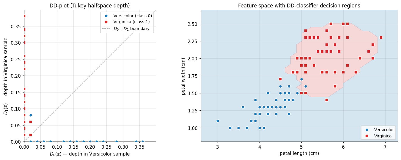
5.1 The DD-classifier

The depth-versus-depth plot, or DD-plot, is the depth-based analogue of a Q–Q plot for two distributions. Given samples $\mathbf{X}_1, \dots, \mathbf{X}_{n_0}$ from a putative class-$0$ distribution $F_0$ and $\mathbf{Y}_1, \dots, \mathbf{Y}_{n_1}$ from class $F_1$, every point $\mathbf{z} \in \mathbb{R}^d$ has two depths:

$D_0(\mathbf{z}) = D(\mathbf{z}; F_{n_0}) \quad \text{and} \quad D_1(\mathbf{z}) = D(\mathbf{z}; F_{n_1}).$

Plotting the pair $(D_0(\mathbf{z}), D_1(\mathbf{z}))$ for each training point in $\mathbb{R}^2$ produces the DD-plot — a low-dimensional summary of how the two classes’ depth structures compare, regardless of the dimension of the original data.

The classifier’s decision boundary in the original feature space $\mathbb{R}^d$ corresponds to the line $D_0 = D_1$ in the DD-plot. When the two depth structures are well-separated, classes appear as distinct clusters in the DD-plot, and the diagonal is a competent decision rule.

This depth-calibration condition holds for halfspace depth on Gaussians (where depth is monotone in Mahalanobis distance, hence in density). The implication: when the elliptical-symmetry assumption is reasonable, the DD-classifier is essentially Bayes-optimal without ever fitting a parametric model — only the empirical depth function is needed. The implementation below computes a DD-plot for the harder Iris pair (Versicolor vs. Virginica) using halfspace depth on the petal-length × petal-width subspace.

The widget below reproduces both views with the live training-accuracy readout. Toggle DD-plot ↔ feature space.

DD-plotFeature space

Versicolor (n=50)Virginica (n=50)|training accuracy: 0.960

In the DD-plot, the diagonal D₀ = D₁ is the decision boundary. Points above the line are classified as Virginica; points below as Versicolor. The two clusters separate cleanly because the Iris petal subspace is nearly linearly separable.

5.2 Multivariate outlier detection

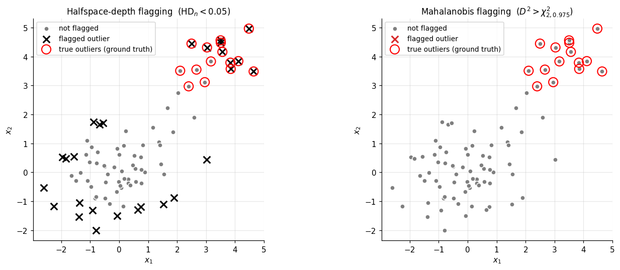
A multivariate outlier is a point that is far from the bulk of a distribution in a sense that respects the bulk’s shape. Mahalanobis distance is the standard tool, but it commits to ellipticity (§3.1). Depth-based outlier detection inverts the problem: outliers are the points with low depth.

The threshold $\alpha$ tunes the rule’s strictness. The most aggressive choice is $\alpha = 1/n$, which flags only convex-hull boundary points; this catches isolated outliers but misses any contamination cluster dense enough to form its own convex region. A more useful default is a fixed $\alpha$ in the $0.02$–$0.10$ range, calibrated either to a clean reference distribution or to the desired fraction of training points one is willing to flag.

A subtle but important property of depth-based outlier rules: they are not fooled by masking — the failure mode where multiple co-located outliers raise their own neighborhood density, inflate the sample covariance toward the contamination direction, and thereby pull their own Mahalanobis distances below the cutoff. Depth-based rules see through masking partially, because the convex-hull and projection structures that define depth do not get pulled toward dense regions of contamination — a contamination cluster of $k$ points can lower the halfspace depth of any point near the bulk by at most $k/n$, regardless of how the cluster is arranged. The honest caveat: when the contamination cluster is dense enough to form its own convex region of significant volume, depth-based flagging can still miss outliers inside that region (they are deep with respect to the cluster, even if shallow with respect to the bulk), and false positives accumulate in the clean bulk’s outer rim.

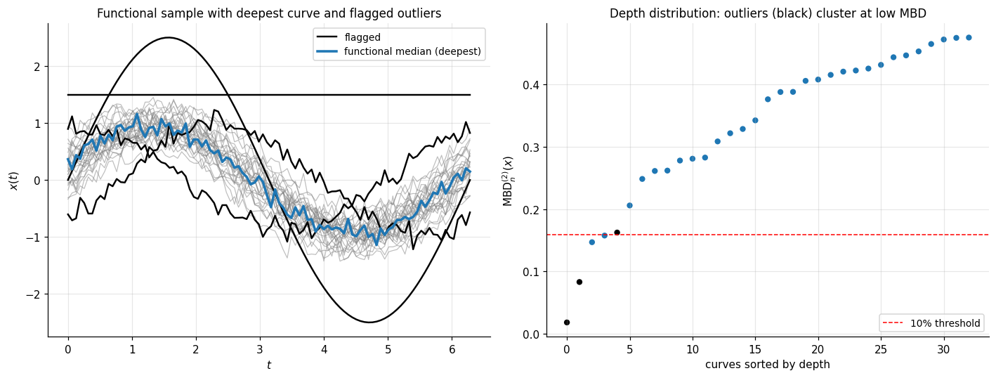
5.3 Functional depth

A functional dataset is a sample of curves $X_1(t), \dots, X_n(t)$, each a function on a common index set $T$. The natural depth analogue is band depth — defined by how often a curve lies between bands generated by other sample curves.

Band depth and modified band depth share the §1.3 axiomatic structure (with appropriate substitutions for functional spaces) and provide center-outward orderings of curves: the deepest curve is the functional median, the most central curve in the sample.

5.4 Depth-weighted M-estimation

A natural generalization of the §4.2 Tukey median is depth-weighted M-estimation: instead of using the deepest point, build an estimator that weights all sample points by a function of their depth. For a weight function $w : [0, 1/2] \to \mathbb{R}_+$,

$\hat{\boldsymbol{\mu}}_w = \frac{\sum_i w\bigl(\operatorname{HD}_n(\mathbf{X}_i)\bigr) \mathbf{X}_i}{\sum_i w\bigl(\operatorname{HD}_n(\mathbf{X}_i)\bigr)}.$

For $w(d) = \mathbb{1}\{d \ge \alpha\}$ this is the centroid of the $\alpha$-trimmed Tukey region, generalizing the median. Continuous weight functions yield smooth estimators that retain a controllable breakdown point (Donoho and Gasko 1992 Theorem 4 gives a $\varepsilon^* \ge 1/(d+1)$ bound under a mild monotonicity condition on $w$).

6. Connections and limits

The depth machinery sits at a junction between the rest of the formalML curriculum and the broader statistical literature on which it is built. This section orients the topic among its neighbors, then lays out the assumptions and computational realities that bound where statistical depth is the right tool and where it isn’t.

6.1 Within formalML

Quantile regression. The §1.1 motivation — that componentwise quantiles fail to give a well-defined multivariate notion of center — is the converse of the quantile regression motivation. Quantile regression handles the conditional multivariate problem (fixing a regressor and asking about the response distribution) by working one quantile level at a time. Statistical depth handles the unconditional multivariate problem (no regressor, just the joint distribution) by collapsing the multidimensional information into a center-outward scalar. The two converge at the multivariate-quantile-regression frontier, where Tukey contours of the residual distribution serve as nonparametric prediction regions.

Conformal prediction. Conformal prediction sets achieve marginal coverage by ranking calibration scores and inverting at the desired quantile. When the score is a multivariate residual, the natural rank is depth rather than componentwise quantile — which gives depth-based conformal prediction: prediction regions whose shapes adapt to the residual distribution’s geometry rather than being committed to coordinate-aligned boxes.

Extreme value theory. EVT and statistical depth are duals: EVT studies the outermost observations, depth studies the innermost. The two combine in multivariate extreme value theory, where shallow-depth observations identify candidate extremes and depth-based contours bound the central mass against which extremes are measured.

Rank tests. Depth provides the multivariate analogue of the rank ordering induced by the empirical CDF. Hodges-Lehmann-style multivariate rank tests built on depth-induced ranks are distribution-free under the elliptical-symmetry assumption and inherit the §4.1 consistency.

Prediction intervals. Multivariate prediction regions inherit the depth-conformal connection: a depth-based prediction region built from the calibration sample’s residual depths is the multivariate analogue of the standard quantile-based univariate prediction interval.

PCA and low-rank methods. PCA finds a lower-dimensional subspace explaining maximum variance; depth maps each point to a scalar quantifying its centrality. The two combine in projection depth (§3.3): the projection-depth value is the worst-case standardized residual over all 1D projections — a robustified version of the leading PCA loading.

Convex analysis. Theorems 1 (axiomatic) and Proposition 1 (convexity of contours) live entirely in the language of supporting hyperplanes, halfspaces, and convex hulls. The convex-analysis toolkit is the natural staging ground for derivations and contour-level-set arguments.

6.2 Cross-site connections

The univariate quantile function on formalstatistics/order-statistics-and-quantiles is the foundational concept that depth generalizes. Empirical-process limit theorems on formalstatistics/empirical-processes — the Vapnik–Chervonenkis Glivenko–Cantelli theorem and Donsker’s theorem on the halfspace VC class — are the structural prerequisites for Theorems 3 and 5 here. The elliptical-symmetry framework on formalstatistics/multivariate-distributions is the assumption under which Theorem 7 (DD-classifier Bayes-optimality) holds. The integrals defining halfspace and band masses live in formalcalculus/multivariable-integration.

6.3 Limits

Sample inefficiency in high dimensions. Statistical depth is a fundamentally geometric construction, and geometry in high $d$ is hostile. The §4.1 consistency rate is dimension-free pointwise — but the uniform rate over depth contours degrades as $O(d / \sqrt{n})$. For practical purposes, depth-based methods are most useful at $d \le 20$. Beyond that, deep-region estimation requires sample sizes that are usually unavailable.

Computational cost. Theorem 6 (Aloupis 2006) is decisive: exact halfspace depth is NP-hard when $d$ is part of the input. The §3.3 projection construction provides a polynomial-time approximation, but the approximation rate $O_p(\sqrt{\log K / K})$ in the number of projections degrades quickly when $K$ must scale with $d$.

Ellipticity assumption in some applications. Theorem 7 (DD-classifier Bayes-optimality) requires elliptical class densities. When the class densities are non-elliptical, the DD-classifier is no longer Bayes-optimal — though it remains a competent classifier and inherits the §4.1 consistency. Practitioners should not lean on the Bayes-optimality result when the data exhibits multimodality, skewness, or heavy non-elliptical structure.

Non-uniqueness of the halfspace median. The Tukey median is in general a set, not a point; uniqueness requires additional symmetry assumptions on $F$. Implementations report the centroid of the deepest level set (§2.3), but this introduces an arbitrary choice that has no statistical justification when the deepest level set has positive volume.

Functional depth is order-dependent. Band depth (§5.3) ranks curves but does not provide a metric structure on the function space — two equally deep curves can be very different in shape. The correct comparison metric (e.g., $L^2$ distance) must come from outside the depth machinery.