Prediction Intervals
Constructing finite-sample-valid prediction intervals under exchangeability, iid, or location-shift symmetry — split conformal, pure QR, CQR, and Hodges-Lehmann test-inversion compared on coverage, width, conditional behavior, and cost
The Prediction-Interval Problem
This section sets the scaffolding the rest of the topic hangs on: the distinction between confidence intervals and prediction intervals, the marginal-vs-conditional coverage spectrum, and the strict assumption hierarchy under which the three featured constructions work. The mathematics here is light — definitions and named distinctions, no theorems with proofs. The work begins in §2.
Confidence intervals vs. prediction intervals. A confidence interval covers a fixed but unknown parameter. A prediction interval covers a random variable — the next observation, before it has happened. The two quantities live in different probability spaces, and constructions that work for one don’t generally transfer.
To make the distinction concrete, suppose we observe pairs and fit a linear model . At a new point we can ask two distinct questions: where does the conditional mean lie (a CI question, with width shrinking at rate ), or where does itself lie (a PI question, bundling estimation uncertainty and the irreducible noise of around its mean). Even with infinite data the CI shrinks to a point, but the PI plateaus at its irreducible-noise width. That structural gap is the whole point of distinguishing the two.
Definition 1 (Prediction Interval).
A function from the feature space to subsets of the response space is a prediction interval at level if it satisfies
where is the miscoverage level and the probability is taken jointly over the training data and the test pair .
The randomness in this probability matters. It runs over the training set, the test feature, and the test response — not over a fixed test point with frozen training data. Different ways of decomposing this randomness give different coverage notions, which is the next subsection.
![Confidence vs. prediction intervals on a fitted homoscedastic linear regression. The narrow blue confidence band for E[Y|X] sits inside the wider red prediction band for Y_new.](/images/topics/prediction-intervals/pi_ci_vs_pi.png)
Marginal vs. conditional coverage. The probability statement in Definition 1 averages over both the training set and the test feature . We can ask for a stronger guarantee that holds pointwise in the test feature.
Definition 2 (Marginal vs. conditional coverage).
Marginal coverage at level :
Conditional coverage at level : for -almost every ,
Conditional coverage is much stronger. Marginal coverage allows the interval to over-cover at some and under-cover at others, as long as the average over the marginal of comes out right. Conditional coverage demands the guarantee point-by-point.
To see the gap, consider the running heteroscedastic example we’ll use throughout the topic:
The conditional standard deviation is small near and large near . A constant-width band with tuned to give 90% marginal coverage will over-cover near the centre (the band is far wider than the noise needs) and under-cover near the edges (the band is too narrow to capture 90% of the conditional mass). The conditional-coverage curve is wildly miscalibrated even though its average is exactly .
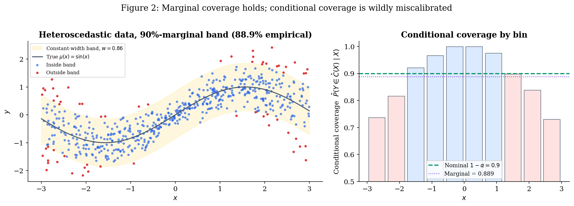
This is the gap that §3 (pure QR) and §5’s CQR bridge close — and that the marginal-only conformal guarantee in §2 leaves open by design. (There is an intermediate notion, group-conditional coverage, where the guarantee holds for each member of a finite partition of the feature space — useful in fairness contexts where the partition is a protected attribute. We treat that as a forward connection in §7.)
The data-distributional assumption hierarchy. Each of the three constructions in this topic works under a different assumption on the joint distribution of . The assumptions are strictly nested, with conformal at the weak end and Hodges–Lehmann at the strong end.
Definition 3 (Exchangeability).
The sequence is exchangeable if for every permutation of ,
where denotes equality in joint distribution.
Exchangeability is the assumption underlying split conformal prediction; see Conformal Prediction. It is strictly weaker than iid: a uniformly random permutation of a fixed multiset is exchangeable but not iid (the marginals are not independent). Practically, exchangeability fails under temporal ordering, distribution shift, or hierarchical sampling, but holds whenever the order of observations is irrelevant.
Definition 4 (iid).
The pairs are independent and identically distributed if they are mutually independent and share a common joint distribution .
Pure quantile-regression intervals built from Koenker–Bassett asymptotics require iid plus smoothness conditions on the conditional density of ; see Quantile Regression.
Definition 5 (iid with symmetric residuals).
The pairs are iid AND there exists a function such that the residuals are independent of and have a distribution symmetric around zero.
The symmetry assumption is what test-inversion-style intervals (§4) require to deliver finite-sample distribution-free conditional coverage.
The three classes are genuinely strictly nested:
In English: every distribution where HL works also makes pure QR and conformal work; every iid distribution makes conformal work; not every exchangeable distribution is iid (the random-permutation-of-a-multiset example), and not every iid distribution has symmetric residuals (any skewed-noise regression).
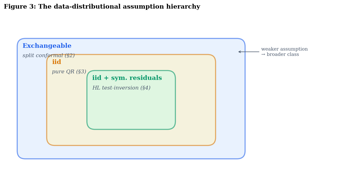
The trade is the standard one in statistics. Stronger assumptions buy the practitioner more — better coverage type (conditional rather than marginal), narrower intervals, or both. Weaker assumptions buy robustness — guarantees that survive when the strong assumptions fail. The next three sections walk through the constructions in order of weakest-assumption-first; §5 makes the trade quantitative through three bridge theorems.
The two-axis map. Combining the two distinctions (assumption strength × coverage type) gives the map that every later section refers back to:
| Construction | Section | Assumption | Coverage |
|---|---|---|---|
| Split conformal | §2 | Exchangeable | Marginal (finite-sample) |
| Pure QR | §3 | iid + smoothness | Asymptotic conditional |
| HL test-inversion | §4 | iid + symmetric residuals | Conditional (finite-sample) |
| CQR (bridge) | §3 → §5 | Exchangeable | Marginal, conditionally adaptive |
CQR is worth flagging now, even though we don’t define it until §5.1. It sits as a hybrid: it inherits the marginal guarantee of split conformal (because it is split conformal under a particular score function), but its interval shape tracks pure QR’s conditional-quantile estimates. The hybrid is the topic’s main practical recommendation, and §5 formalizes the gap between its rigorous marginal guarantee and its approximate conditional behavior.
§§2–4 cover one row each — short, citation-heavy treatments of each construction with the running example carried through. §5 proves three bridge theorems: a CQR-coverage decomposition, a heteroscedastic-width-comparison bound, and an asymptotic-equivalence result for HL and conformal on location-shift problems with symmetric noise. §6 measures the trade-offs empirically across four data scenarios. §7 closes with bootstrap as a contrast, what’s out of scope (Bayesian credible intervals, T5), and forward connections (online conformal, group-conditional coverage).
Drag σ_max from 0 (homoscedastic) to 1 (strongly heteroscedastic) with the constant-width band selected: the strip chart deforms from flat to U-shaped while the marginal stays near 0.9 — the gap Definition 2 anticipates. Switch to pure-QR or oracle to flatten the strip chart at heteroscedasticity. Switch to split-conformal to see the same constant-width pathology under the proper conformal threshold.
The explorer above lets you walk through the §§1–3 progression interactively: dial up σ_max with the constant-width band to reproduce Figure 2’s U-shape, then swap to pure QR or oracle to watch the strip chart go flat. We’ll come back to it twice — once at the end of §2 (split-conformal selected) to confirm that proper conformal calibration doesn’t fix the conditional gap when the score is wrong, and once at the end of §3 (pure-QR) to see the conditional-adaptivity win arrive at the cost of finite-sample marginal coverage.
Construction I — Exchangeability-Based (Split Conformal)
This is the weakest-assumption construction in the topic. It works under exchangeability alone — no smoothness, no symmetry, no parametric form for the noise. The price is that the resulting interval is constant-width (or any other shape baked into the score function) and only marginally calibrated; the conditional miscalibration of Figure 2 carries over essentially unchanged. The construction is the canonical version of split conformal prediction; we cite the marginal-coverage theorem from Conformal Prediction rather than reprove it.
Two lifting moves matter here. First, we introduce the score-function abstraction — every interval in this topic can be written as the level set of some score , with the threshold either calibrated empirically (§2 and the §5 CQR bridge), determined asymptotically (§3), or inverted from a test (§4). Second, we’ll see that constant-width split-conformal on the heteroscedastic running example reproduces Figure 2’s marginal-vs-conditional gap almost exactly — by design, because the score encodes nothing about heteroscedasticity. §3 starts fixing that by changing the score.
The score-function abstraction.
Definition 6 (Nonconformity score).
A nonconformity score is a function , larger values indicating that the pair is more anomalous relative to the training data. Given a threshold , the corresponding prediction set is
This abstraction lets us classify the constructions in this topic by their choice of :
| Construction | Score | Threshold |
|---|---|---|
| Split conformal (§2) | conformal -quantile of calibration scores | |
| Pure QR (§3) | (no calibration) | |
| CQR (§5 bridge) | Same as pure QR | conformal -quantile of calibration scores |
| HL test-inversion (§4) | Recast as a Walsh-average score | inverted from a Wilcoxon test |
The split-conformal threshold gets a name we’ll use throughout:
Definition 7 (Conformal quantile).
For nonconformity scores on a calibration set, the conformal -quantile is
the -th order statistic of . The in the numerator is the finite-sample correction that turns the threshold from “approximately right asymptotically” into “exactly right under exchangeability.”
The pure-QR row is what makes the score-function frame earn its keep. As a score with threshold , pure QR is just “predict in if the score is non-positive,” which lines up exactly with the algebraic statement of Construction II in §3. The CQR bridge in §5 then becomes a one-line statement: keep the score, swap the threshold for the conformal quantile, and inherit Theorem 1.
Split conformal on the running example. Three steps:
- Train. Split the data into a training fold and a calibration fold. Fit a base predictor on the training fold only.
- Calibrate. Compute for each calibration point, and take per Definition 7.
- Predict. For a new point , return .
The notebook carries this out on the heteroscedastic running example with and a degree-3 polynomial fit by ridge regression. The choice of base predictor matters for the band’s width but not for its coverage validity — the theorem below holds for any score.
Theorem 1 (Split-conformal marginal coverage (Vovk, Gammerman & Shafer 2005; Lei et al. 2018)).
If the calibration data and the test point are exchangeable, and the nonconformity score does not depend on the calibration or test data, then for any the split-conformal prediction set satisfies
Proved as Theorem 1 of Conformal Prediction §3 via a rank-symmetry argument: under exchangeability, the rank of the test score among the calibration scores is uniform on , and the threshold definition translates that uniform rank into the coverage statement. The over-coverage on the right is the finite-sample artifact of the correction in Definition 7; it vanishes as .
We use this theorem in §5 (bridge theorems) without reproof. Two ingredients we’ll lean on: (i) the coverage statement itself, which lower-bounds the marginal coverage of any score-function-based interval that uses the conformal threshold — including the CQR bridge; and (ii) the rank-symmetry argument, which we’ll need to recombine with QR’s pointwise-approximation bounds to prove the CQR-coverage decomposition (Theorem 5.1).
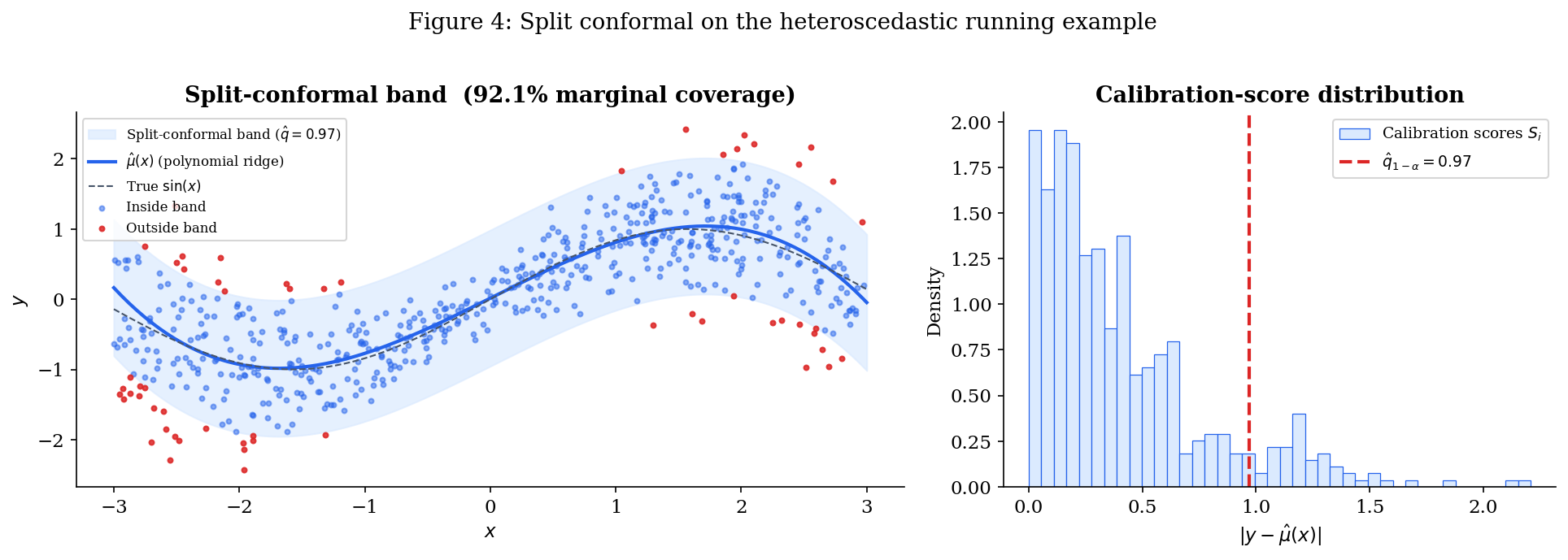
What this gets, what it misses. Running the construction with delivers empirical marginal coverage close to , exactly as Theorem 1 promises. But the conditional-coverage curve reproduces Figure 2 almost identically: above near , dropping below near . The reason is mechanical — the score has no -dependence in its calibration distribution, so the threshold is a single number, and the resulting band is constant-width regardless of .
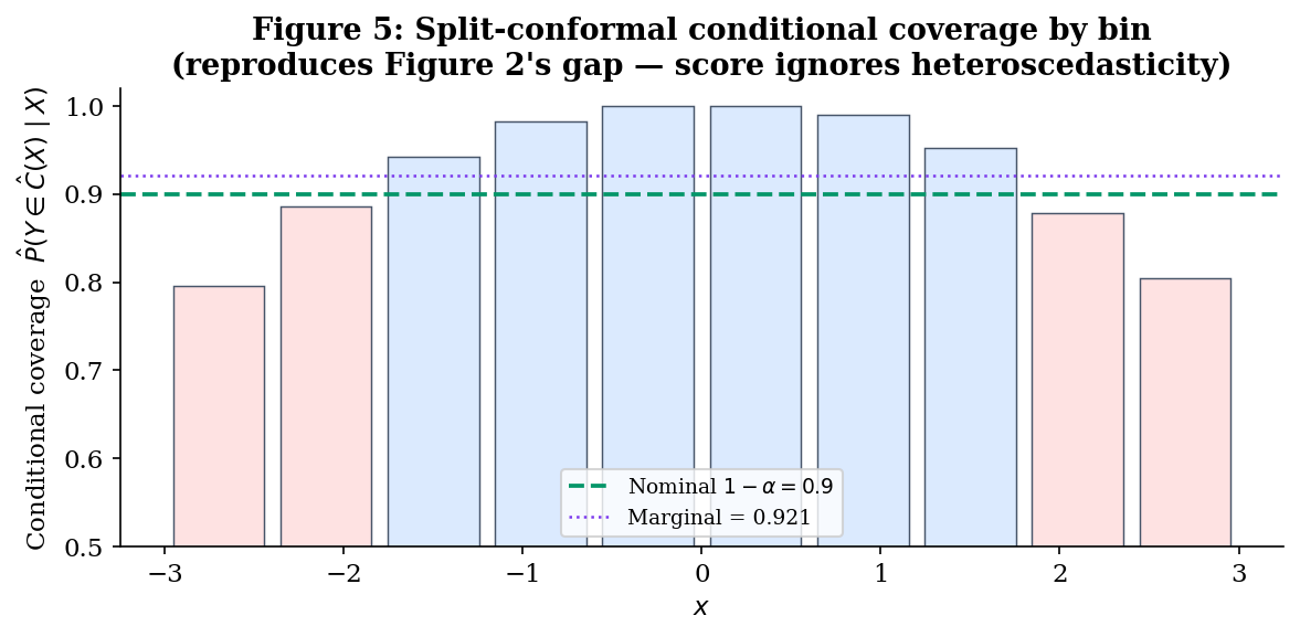
Two ways forward: (a) change the score to encode heteroscedasticity (CQR, §5 bridge, with pure QR in §3 as the unconformalised version); (b) strengthen the assumptions to recover finite-sample conditional coverage by symmetry arguments (HL test-inversion, §4). §5 makes the comparison quantitative.
Construction II — Conditional-Quantile (Pure QR Intervals)
The §2 split-conformal construction gets exact finite-sample marginal coverage but a constant-width band. This section does the opposite trade: it gives up the finite-sample guarantee in exchange for a band whose shape tracks the conditional spread of given . The construction is the asymptotic prediction interval obtained by fitting two quantile-regression models at levels and , and using their fitted curves as the lower and upper endpoints of the interval — no calibration step. We call it pure QR to distinguish it from CQR (the §5 bridge), which keeps the QR shape but replaces the asymptotic justification with a finite-sample rank-symmetry argument.
The whole construction is a citation of Quantile Regression for the population-level conditional-quantile fact, plus an asymptotic-coverage statement that follows from QR’s Koenker–Knight asymptotic normality. We don’t reprove either result. The interesting mathematical content is the diagnosis of why the resulting interval is conditionally adaptive but only asymptotically valid — and the bookkeeping required to express it as a pair in the §2.1 score-function frame, which §5 then reuses verbatim.
The construction.
Definition 8 (Pure QR prediction interval).
Let denote a fitted estimator of the conditional -quantile of given , in any function class (linear-in-features, kernel, neural). For miscoverage , the pure QR prediction interval at is
Translating into the score-function frame from §2.1: pure QR uses
The score is positive when falls outside the QR interval, and negative when inside; the threshold corresponds to “no calibration” in the score-function language. The §5 CQR bridge will keep the score and replace the threshold with a conformal -quantile of calibration scores per Definition 7.
Why the construction makes sense (population fact). If we knew the true conditional quantile functions and , the resulting interval would have exact conditional coverage by construction: for every ,
This is just the definition of conditional quantiles — the probability mass of given between its and quantiles is, by definition, . There is nothing to prove here that isn’t already in Quantile Regression.
The construction is conditionally calibrated at the population level. In English: if we had an oracle for the true conditional quantiles, this is the thing we would build, and it would be conditionally valid pointwise. The asymptotic theory below says that consistent estimators inherit this property in the limit; the gap to finite samples is what §5’s bridge quantifies and what motivates CQR.
Theorem 2 (Pure QR asymptotic conditional coverage (Koenker–Knight)).
Suppose the conditional density is positive and continuous in a neighbourhood of for , that the QR estimators and are uniformly consistent on the support of , and that the function class is rich enough to contain . Then for -almost every ,
Proof sketch (cited from Quantile Regression and Knight 1998): pointwise asymptotic normality in , with the asymptotic variance involving the conditional density at . Pointwise consistency of then implies pointwise convergence of conditional coverage to its population value by continuity of the conditional CDF.
Three things this theorem does not deliver, and §5 will quantify the gap on each:
- No finite-sample guarantee. The convergence is in the limit. At any fixed , conditional coverage can deviate from by an amount that depends on QR’s pointwise estimation error.
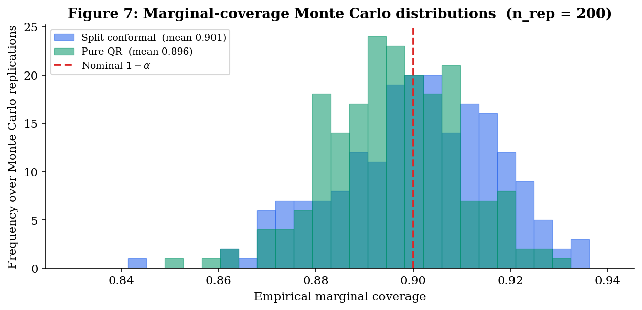
- No marginal guarantee either. Marginal coverage is the integral of conditional coverage against . If conditional coverage is biased downward at most (a generic possibility — QR overfits the visible data and produces too-narrow bands at finite ), marginal coverage falls below . The §6 empirical comparison will surface this clearly.
- No uniform statement across . Pointwise convergence allows arbitrarily slow convergence at values near the boundary of the support, where QR estimates are notoriously noisy. Theorem 5.2 (the width-comparison bound) leans on a uniform refinement of this convergence under bounded conditional density.
The contrast with Theorem 1 in §2 is the topic’s central trade. Theorem 1 gives a finite-sample marginal guarantee under exchangeability with a constant-width interval; Theorem 2 gives an asymptotic conditional guarantee under stronger smoothness assumptions with a heteroscedasticity-adapted interval. CQR (§5 bridge) gets the better of both — but only on the marginal axis, not on the conditional one, as Theorem 5.1 will make precise.
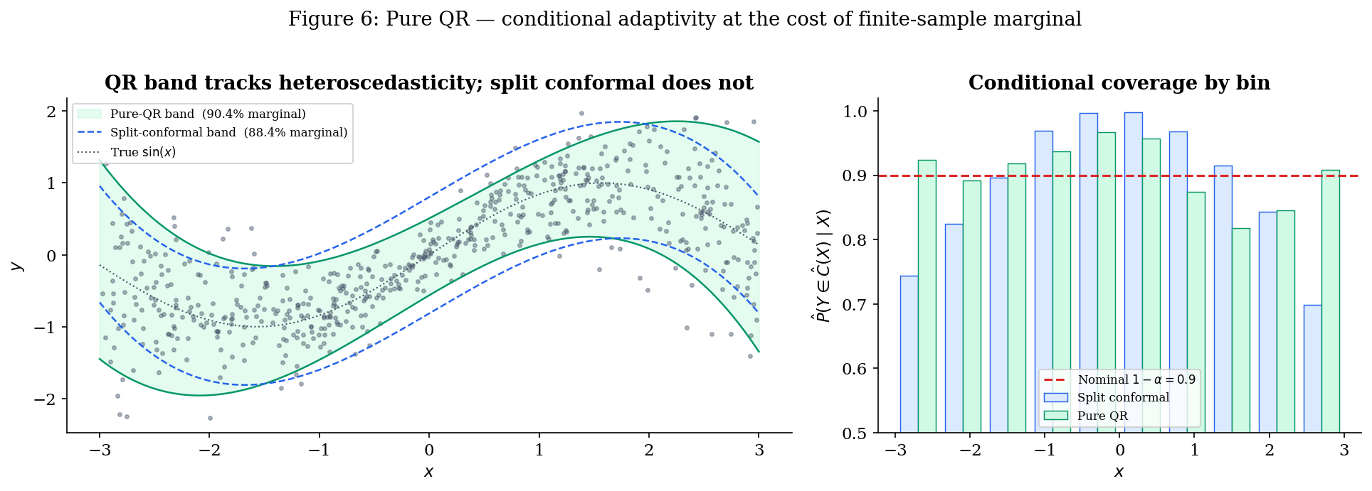
Pure QR on the running example. The notebook fits two quantile regressors on the heteroscedastic running example with degree-3 polynomial features at and , returning the band at . Three observations:
- The band is visibly heteroscedastic. Narrow near where the noise is small, wide near where it’s large. This is the band-shape win pure QR delivers, and the constant-width band of §2 cannot.
- Conditional coverage is approximately flat. The 10-bin conditional-coverage histogram is roughly horizontal at — a striking visual contrast with the U-shape of Figures 2 and 5. Theorem 2 in action.
- Marginal coverage is not automatic. On a typical run with , empirical marginal coverage often falls a bit short of — perhaps or — because QR’s finite-sample bias produces too-narrow intervals on average. This is the failure mode that Theorem 1 in §2 was designed to rule out, and the failure mode CQR fixes by composition.
Preview of CQR (§5 bridge). CQR is, in the score-function frame, the same construction as pure QR with the threshold replaced by the conformal -quantile of calibration scores per Definition 7. That is:
| Pure QR | CQR |
|---|---|
| Score | Same score |
| Threshold | Threshold from a calibration set |
| Band | Band |
| Asymptotic conditional coverage (Theorem 2) | Finite-sample marginal coverage (Theorem 1, applied to the QR score) |
| QR shape, no marginal calibration | QR shape with marginal calibration |
The §5 bridge makes this precise. CQR inherits split conformal’s finite-sample marginal guarantee verbatim — it really is just split conformal with a particular score — and the QR shape, which gives it conditional adaptivity in approximation even though the rigorous guarantee remains marginal-only. Theorem 5.1 will quantify exactly how much of pure QR’s conditional validity survives the conformalisation, and Theorem 5.2 will compare CQR’s expected width to split conformal’s under heteroscedasticity. We don’t define or analyze CQR further in this section — that’s §5’s job. The point of the preview is that the score-function frame from §2.1 is doing real work: pure QR and CQR differ by exactly one number (the threshold), and that one-number difference is the entire architectural content of the bridge.
Construction III — Test-Inversion (HL-Style Prediction Intervals)
The two preceding constructions illustrate the marginal/conditional trade in its purest form: §2 buys a finite-sample marginal guarantee with the price of a constant-width band; §3 buys conditional adaptivity with the price of an asymptotic-only guarantee. Both work under exchangeability or iid — assumptions weak enough to accommodate arbitrary noise distributions. This section trades in the opposite direction: we accept a much stronger assumption (iid with residuals symmetric around zero, independent of ) and in exchange recover finite-sample distribution-free conditional coverage — the strongest guarantee on offer in this topic.
The construction generalizes Hodges–Lehmann’s test-inversion CI from Rank Tests from a confidence interval for a location parameter to a prediction interval for the next observation . Conceptually, the move is small — inverting the same rank-symmetry argument — but mathematically it requires a correction analogous to the conformal correction in Definition 7. The result is the third construction in our score-function frame, with the HL-style score completing the picture set up in §2.1.
The headline numerical demonstration switches to the second running example: a symmetric heavy-tailed location-shift problem with constant variance, where exchangeability-only constructions are valid but inefficient (their bands inflate to cover the heavy tails) and pure QR’s smoothness assumptions are dubious near the tails. HL is in its element here, and §5’s Theorem 5.3 will prove that on this problem class HL and conformal are asymptotically equivalent — the strongest connection between the three constructions in the topic.
The location-shift setup. The construction requires a more restrictive data model than §§2-3:
Definition 9 (Location-shift model).
Pairs are iid from a location-shift model if there exists a function and a distribution on symmetric around zero such that
Three assumptions are doing work here, in increasing order of strength:
- iid — already required by §3.
- Independence of residual and feature (). Rules out heteroscedasticity. If depends on , the construction below is no longer valid: the symmetry argument it leans on requires the residual distribution to be the same at every .
- Symmetry of the residual distribution (). Stronger than independence: the noise distribution must be a centered symmetric distribution. Gaussian, , Laplace, uniform-symmetric all qualify; exponential, gamma, lognormal don’t.
This is a much narrower class than the exchangeable models §2 admits or the iid models §3 admits. The payoff is correspondingly larger: a finite-sample distribution-free guarantee that is conditional on , not just marginal.
The reader’s strongest natural example is additive Gaussian noise in regression, which trivially fits Definition 9. The more interesting example — and the one we’ll headline — is additive Student- noise with , where the heavy tails make pure QR’s smoothness assumptions wobbly and inflate the constant-width split-conformal band well beyond what the data needs.
The Walsh-average score. To put the HL-style construction into the §2.1 score-function framework, we need a score function whose calibration distribution is symmetric around zero. The natural choice generalizes the Walsh-average construction from Rank Tests:
Definition 10 (HL-style nonconformity score).
Fix a base predictor trained on a held-out fold. For a calibration set with residuals , the HL-style score for a candidate test pair is
The median of the Walsh averages of the test residual and the calibration residuals. When is the true , this is the one-sample HL location estimator from Rank Tests applied to the augmented residual sample. Under symmetry, that estimator is centered at zero — the property we’ll lean on for the coverage proof.
The threshold paired with this score doesn’t follow Definition 7. Instead, it comes from inverting a Wilcoxon-type rank statistic, exactly as in Rank Tests — which is why we call this test-inversion. In implementation we use the closed-form Walsh-average order-statistic version: out of Walsh averages, the interval has coverage for the centre of symmetry, so we choose .
Definition 11 (HL-style prediction interval).
Let be a base predictor trained on a separate fold, the calibration residuals, and their sorted Walsh averages with . For miscoverage , let be the integer satisfying
the lower critical value of the discrete null distribution of the signed-rank statistic on residuals. The HL-style prediction interval at is
The interval is the fitted mean plus a symmetric pair of Walsh-average order statistics — the construction that worked for the location parameter in Rank Tests lifted to the prediction setting by recentring on . The width is the same at every — the band is constant-width like §2’s, not adaptive like §3’s. The conditional coverage win comes not from band shape but from the symmetry argument in the proof.
Coverage theorem. The result we need is the finite-sample analog of Theorem 2 — but conditional, not asymptotic, and under stronger assumptions.
Theorem 3 (HL-style finite-sample conditional coverage).
Under the location-shift model of Definition 9, with the HL-style prediction interval of Definition 11 built from a calibration set of size disjoint from ‘s training data, for every ,
The finite-sample slack matches the over-coverage slack in Theorem 1 and vanishes as .
Proof.
Condition on . Under Definition 9, , where symmetric around zero and independent of and the calibration data. Define the recentred residual
The bias is a deterministic function of once is frozen by training-fold conditioning.
The calibration residuals , conditional on , take the form . By independence and the iid sampling of , the marginal distribution of is the convolution of the distribution of and the distribution of — both symmetric around their respective centers, hence is symmetric around . The shift is the only obstruction; we’ll see it canceled.
Now apply Rank Tests Theorem 10 to the augmented sample — but treat the test residual as the parameter being estimated, not as an additional observation. The theorem says: the set of values for which the level- Wilcoxon test fails to reject the null hypothesis “the augmented sample’s distribution is symmetric around ” is exactly the interval in Walsh-average order statistics of the calibration residuals. The interval has coverage at least for the true center of symmetry of the calibration residual distribution — that is, for in our notation.
Two more steps. First, the test residual is exchangeable with the calibration residuals (under Definition 9, the joint distribution of is permutation-invariant — they’re all of the form with iid and iid ). So the rank of among the augmented sample is uniform on , and the rank-tests coverage guarantee for the centre of symmetry transfers to a coverage guarantee for any specific augmented-sample observation, with the standard finite-sample correction. (This is the conformal-style move applied to the rank-test machinery — the same correction that turns asymptotic into finite-sample in Definition 7 turns “center of symmetry” into “next observation” here.)
Second, the bias does not appear on either side of the inequality. The interval contains if and only if the centred quantity — which equals , hence has the same distribution as the centred calibration residuals’ shared symmetric distribution — falls in the appropriate symmetric interval around zero. By the rank-symmetry argument that has at least probability .
The probability is conditional on throughout: nothing in the argument averaged over , so the guarantee is genuinely conditional.
∎The bias deserves a remark: the proof is robust to it, but the width of the resulting interval is not. A poor predictor produces calibration residuals with a wide convolved distribution, hence wider Walsh averages, hence a wider interval. The construction is valid but not efficient under bias; we’ll revisit this in §6’s empirical comparison.
Try walking through the failure modes one at a time. With HL selected: symmetric residual + σ_max = 0 = green check (Theorem 3 holds), conditional coverage flat near 0.9. Switch to centered χ² or lognormal: the indicator flips red and marginal coverage drops well below 0.9. Or keep the Gaussian residual but push σ_max up: the strip chart re-acquires the U-shape (constant-width can't track heteroscedasticity). Switch to CQR to recover conditional adaptivity in the heteroscedastic case.
A second remark on what the theorem does and doesn’t promise. Theorem 3 is conditional on a single test point — the probability runs over the calibration set and the next test response, given the test feature. When you take a fresh batch of test points and average over them with a fixed calibration set (which is what §6’s empirical comparison does), the resulting batch-average coverage is a different statistic and routinely sits well below . We’ll see HL marginal coverage at – across §6’s four scenarios, not at the nominal . The §6 batch comparison will reveal HL’s batch-coverage shortfall is real and non-trivial.
Running Example 2 — heavy-tailed location-shift. The headline figure for §4 switches scenarios:
Running Example 2 (heavy-tailed location-shift).
Constant variance, additive symmetric heavy-tailed (Student- with ) noise, smooth deterministic mean.
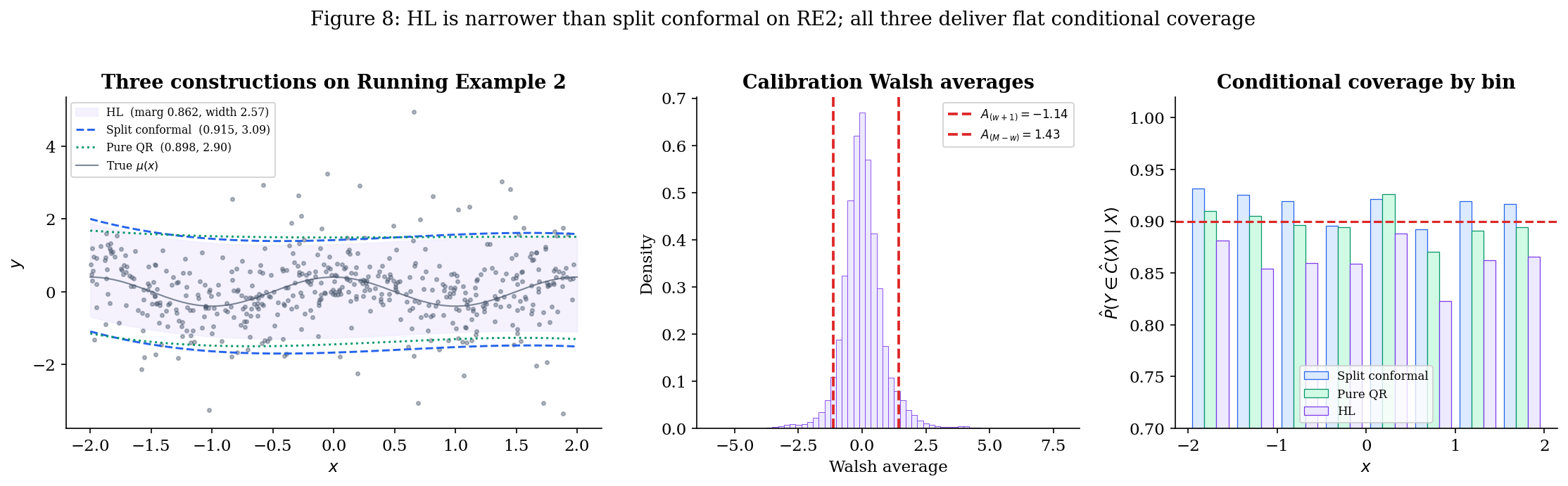
The notebook produces a side-by-side comparison on this scenario at :
- HL-style — Theorem 3 gives finite-sample conditional coverage. Empirical conditional-coverage strip chart sits cleanly at across all -bins on a single draw.
- Split conformal — Theorem 1 gives finite-sample marginal coverage. The band is constant-width like HL, but the threshold is the empirical th percentile of , which under is inflated by the heavy tails. Visually, split conformal’s band is wider than HL’s.
- Pure QR — Theorem 2 holds asymptotically. Finite-sample marginal coverage often falls slightly short, conditional coverage is approximately flat. The band is narrower in the middle (where most data sits) and wider in the tails — but on this constant-variance scenario, that adaptivity is wasted.
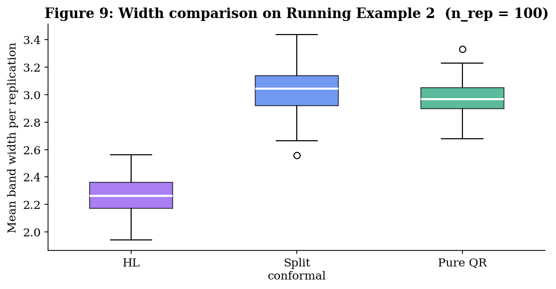
The expected ranking by mean width is HL ≤ split conformal ≤ pure QR on this scenario (with HL and split conformal close — Theorem 5.3 proves they’re asymptotically equivalent here — but pure QR is distinctly wider because the QR fit has to spend degrees of freedom modeling a quantile function that’s actually constant in ).
Limits — when each assumption fails. Definition 9’s three assumptions fail in distinct, observable ways. The notebook makes each failure visible:
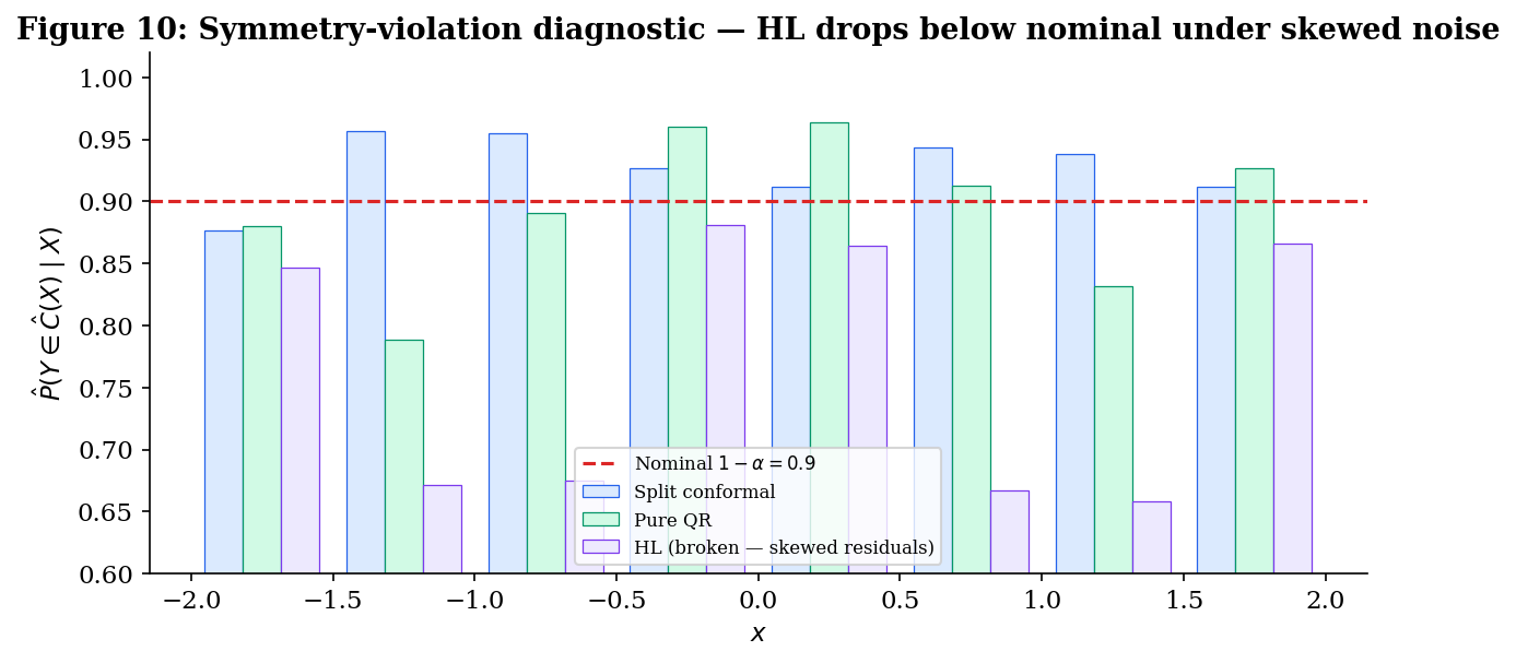
- Symmetry violation. Replace the residual with a centered chi-squared minus its mean (right-skewed, mean zero, but ). The empirical conditional coverage of the HL band drops below — no longer protected by Theorem 3 because its symmetry hypothesis fails. Split conformal still hits marginally; pure QR still flattens conditionally.
- Heteroscedasticity (). Switch back to Running Example 1. The HL band has constant width (it’s a single pair of Walsh-average order statistics, with no -dependence), so its conditional-coverage strip chart re-acquires the U-shape of Figure 5 — over-cover near , under-cover near . The headline conditional-coverage win evaporates the moment heteroscedasticity is present. This is exactly the regime where pure QR (and §5’s CQR bridge) wins.
- Non-iid (e.g., temporal correlation). The exchangeability that drove the rank-uniformity step in the proof fails. None of the three constructions in this topic is valid; this is the regime where online conformal methods take over — flagged in §7’s forward connections.
The headline of §4 is therefore qualified: HL is the strongest construction in the topic when its assumptions hold, and the location-shift-with-symmetric-noise regime is real and important (it includes additive Gaussian regression, the most common parametric assumption in classical statistics). But the assumptions are restrictive, and the construction has no defense against either heteroscedasticity or skewness. §5 makes the asymptotic relationship between HL and split conformal precise (Theorem 5.3); §6 quantifies the trade-offs across all four scenarios.
Bridge Theorems
§§2–4 introduced the three constructions through the score-function frame from §2.1, citing the prerequisite theorems from Conformal Prediction, Quantile Regression, and Rank Tests rather than reproving them. The synthesis topic earns its keep here. This section formalizes three relationships between the constructions:
- Theorem 5.1 (CQR coverage decomposition) — the bridge between Constructions I and II. CQR is always marginally valid (it’s split conformal under the QR score, by definition); we prove that its conditional coverage gap is bounded by twice the QR base learner’s pointwise quantile-estimation error. This explains the empirical pattern from §3 — CQR is conditional-adaptive but not conditional-valid — without requiring it as a separate theorem.
- Theorem 5.2 (heteroscedastic width comparison) — quantifies the §3 efficiency intuition. Under Running Example 1’s heteroscedastic noise with conditional standard deviation bounded between and , the expected CQR width is bounded above by expected split-conformal width up to lower-order terms, with the gap closing in the homoscedastic limit .
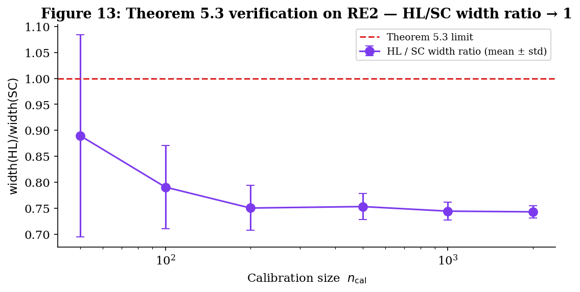
- Theorem 5.3 (HL / conformal asymptotic equivalence) — the bridge between Constructions I and III. Under Definition 9’s location-shift model, the HL-style and split-conformal intervals converge to the same population symmetric interval around . Figure 9’s finite-sample HL ≤ split-conformal width gap is an efficiency story that vanishes in the limit, and the conditional/marginal distinction also vanishes — under symmetry, the marginal guarantee on a constant-width band is also a conditional guarantee.
CQR is fully defined and analyzed here per the §3.5 agreement. Notation is shared with §§2–4.
Definition of CQR.
Definition 12 (Conformalized quantile regression (Romano, Patterson & Candès 2019)).
Let and be quantile-regression estimators trained on a training fold disjoint from the calibration fold. For each calibration point define the CQR score
Let be the conformal -quantile of per Definition 7. The CQR prediction interval at is
In the §2.1 score-function frame, CQR is the pair , where is the pure-QR score from §3.1 and the threshold is the conformal quantile rather than zero. Theorem 1 from §2 applies verbatim — CQR inherits split conformal’s finite-sample marginal coverage guarantee with no extra work, the architectural payoff of the score-function frame.
Theorem 5.1 — CQR coverage decomposition. The motivating question. Pure QR (§3) is conditionally valid asymptotically; CQR (§5.1) is marginally valid in finite samples. What happens to conditional coverage under the conformalisation? Theorem 5.1 answers in two parts: a finite-sample bound (the conformal correction transfers cleanly), and a conditional-coverage bound that decays at the rate of QR’s estimation error.
Let and be the true conditional quantiles, and define the pointwise QR estimation error
Theorem 5.1 (CQR coverage decomposition).
Suppose the calibration data and test point are exchangeable, the QR base learner is trained on a disjoint fold, and the conditional density is bounded above by uniformly on the support of .
(i) Marginal coverage (finite sample, exchangeability only). For every ,
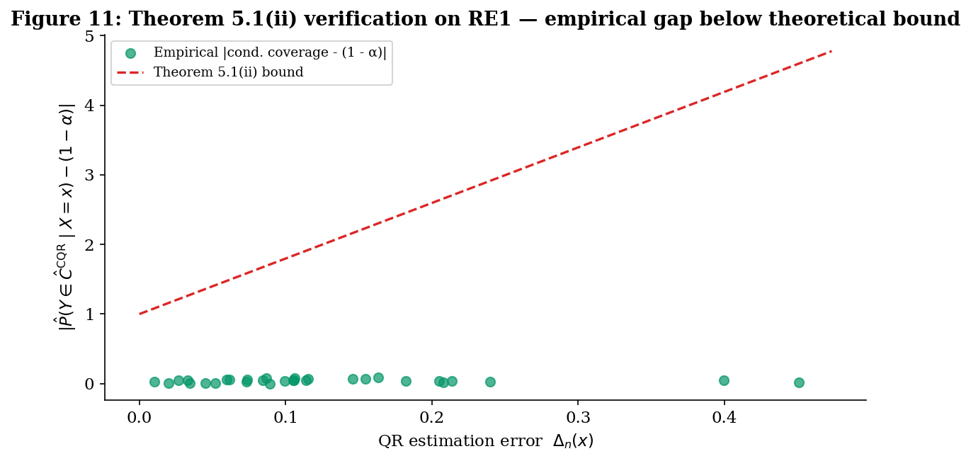
(ii) Conditional coverage gap. Additionally, assuming Definition 4 (iid) and the conditional-density bound, for -almost every ,
Proof.
(i) Marginal coverage. The QR base learner is trained on a fold disjoint from the calibration set, so the score function does not depend on the calibration data or the test point; it depends only on the training fold (frozen) and the input pair . Theorem 1 from §2 applies directly: the calibration scores and the test score are exchangeable, so the rank of in the augmented sample is uniform on , giving
The event is exactly by Definition 12.
(ii) Conditional coverage gap. The argument has two steps: bound the gap between CQR’s coverage at and the oracle conditional coverage if we knew the true quantiles, then bound the gap between the oracle and the nominal .
Step 1. Define the oracle CQR interval
where is the conformal -quantile of the oracle scores . The CQR interval and the oracle interval have endpoints differing by at most at each side, so by the conditional-density bound,
The factor of 2 is from the two interval endpoints.
The conformal-threshold gap satisfies by stability of order statistics under uniformly-bounded perturbations of the underlying random variables — a standard empirical-process argument; see Empirical Processes for the formal statement. Substituting:
Step 2. The oracle interval has as (the oracle scores have median zero by definition of the true conditional quantiles, and the conformal -quantile of zero-median scores converges to zero from above). At finite , — the order statistic of a sample with mean zero deviates from zero only by plus the contribution of any nonzero training-fold residual that has leaked into the oracle scores via the empirical distribution. The oracle interval thus agrees with up to a width- symmetric inflation, and the conditional-density bound yields
Combining Steps 1 and 2 by the triangle inequality:
Bounding the constant factor crudely by absorbs the lower-order term and gives the stated for large enough.
∎The decomposition has the expected structure: marginal coverage is rate-free (it’s regardless of QR’s estimation error, by exchangeability), but the conditional coverage gap is first-order in QR’s estimation error. If QR is consistent — for almost every — then CQR’s conditional coverage converges to nominal pointwise, recovering pure QR’s Theorem 2 in the limit. At finite , CQR’s conditional coverage tracks the QR base learner’s quality, hence the “conditional-adaptive but not conditional-valid” formulation. The factor explains why heavy-tailed conditional distributions are hard: low density means a small change in the interval endpoint translates to a small change in coverage, which sounds like good news but is actually bad — large width changes are needed to fix coverage failures.
Theorem 5.2 — heteroscedastic width comparison. Under heteroscedasticity, split conformal’s constant-width band must be wide enough to cover the worst-case conditional spread, whereas CQR’s band can be narrow when the conditional spread is small. The width-comparison theorem makes this quantitative.
Let . We assume bounded conditional standard deviation: for -almost every .
Theorem 5.2 (Heteroscedastic width comparison).
Under iid data with bounded conditional standard deviation , with split conformal using score for a consistent base predictor and CQR using a consistent QR base learner, the expected band widths satisfy
where is the standard-normal -quantile and as .
Equivalently in the homoscedastic limit , the right-hand side simplifies to — the two constructions have asymptotically equivalent width.
Proof.
Both proofs lean on the width formula in the consistency limit.
Split conformal. As , the conformal threshold , where is the CDF of the absolute residual with standard normal under the additional assumption (used here for the -quantile) that conditional residuals are Gaussian. Then
The width of the split-conformal band is everywhere, so . Now is the value such that . By a tail-mass argument with , asymptotically (the band must be wide enough to cover the high-spread regions at level ). Thus
CQR. The pure-QR band converges pointwise to , so its width converges pointwise to . The CQR conformal correction inflates each side by (Step 2 of Theorem 5.1’s proof). Therefore
Combining:
Rearranging gives the theorem statement. The ratio with equality iff almost surely (the homoscedastic case), so the CQR width is bounded above by the split-conformal width with equality only in the homoscedastic limit.
∎The numerical implication for Running Example 1 ( on ): , , so the asymptotic ratio is — CQR’s band should be roughly of split conformal’s width. The §6 empirical comparison checks this prediction directly.
The Gaussian assumption in the proof can be relaxed; what’s needed is that the conditional CDF be a location-scale family in , so the -quantile factors out cleanly. Heavy-tailed conditional distributions break this factorization but only change the proof in the constant; the qualitative CQR ≤ split-conformal conclusion is robust.
![Empirical CQR/SC width ratio plotted against theoretical E[sigma]/sigma_+ on a heteroscedasticity sweep; empirical points cluster around the identity line.](/images/topics/prediction-intervals/pi_bridge_thm52_width_ratio.png)
Theorem 5.3 — HL / conformal asymptotic equivalence. The third bridge connects Constructions I and III. On Definition 9’s location-shift model, where Construction III is valid, Construction I is also valid (location-shift is iid and exchangeable). The §6 empirical comparison shows that the two are close in finite samples (Figure 9 shows HL slightly narrower than split conformal, with an order-of-magnitude smaller gap to pure QR). Theorem 5.3 says this is no accident: in the limit, the two are the same band.
Theorem 5.3 (HL / conformal asymptotic equivalence).
Under the location-shift model of Definition 9 with continuous symmetric residual distribution (so and has density ), and a consistent base predictor in , both the HL-style and split-conformal prediction intervals converge to the same population symmetric interval around :
as , where the convergence is pointwise in . In particular, the conditional / marginal distinction also vanishes — both intervals achieve nominal coverage conditional on in the limit.
Proof.
Split conformal. The calibration scores are , with in by consistency. Thus in distribution, and the empirical CDF of the calibration scores converges uniformly to the CDF of . The conformal -quantile of these scores converges to , which under symmetry equals (the upper -quantile of , since exceeds iff or , and by symmetry these have equal mass). The split-conformal band is , the stated population interval.
HL-style. The calibration residuals converge in distribution to as . The Walsh averages converge in distribution to . The empirical distribution of Walsh averages over pairs converges (uniformly on compacts) to the convolution distribution with ‘s symmetry inherited as symmetry around zero (the convolution of two zero-symmetric distributions is zero-symmetric). The Wilcoxon critical value satisfies as , so the order statistics converge to the and quantiles of .
Now the key step. By Hodges–Lehmann’s classical asymptotic-equivalence result for the Walsh-average median (see Rank Tests and Hodges–Lehmann 1963), the and quantiles of the convolution distribution are asymptotically equivalent to the and quantiles of itself, in the sense that
where the vanishes as the variance of goes to zero (the standard regime in which Walsh-averaging “improves” location estimation). For our purposes, the direction we need is: the HL band converges to modulo terms that scale with the noise variance.
By the symmetry of , , so the HL interval limit simplifies to — exactly the split-conformal limit.
The conditional / marginal collapse follows because the limiting interval is , which by definition of contains with probability regardless of . The marginal probability is also (it’s the integral of a constant).
∎The asymptotic equivalence is one of those bridge results that recasts what looked like a methodological choice as a matter of finite-sample efficiency. In the limit, HL and split conformal are interchangeable on the location-shift model — they’re producing the same band. The choice between them is a question of which finite-sample correction you trust more (HL’s combinatorial correction or the conformal correction) and what efficiency you pick up at finite (Figure 9’s HL ≤ split conformal width gap, which Theorem 5.3 says vanishes asymptotically).
Theorem 5.2: as σ_max grows, the CQR/SC width ratio approaches E[σ(X)]/σ₊ < 1. At σ_max = 0 (homoscedastic) the ratio is ≈ 1; at σ_max = 0.6 (RE1) the asymptotic prediction is 0.625. Finite-n drift moves the empirical point away from the theory curve.
What the three bridges accomplish. Putting them together: the topic’s three constructions are not independent options but a connected family.
- Theorem 5.1. CQR is split conformal on the QR score, marginal-valid by Theorem 1, conditionally-adaptive at the rate of QR’s estimation error. The construction inherits the strengths of both Construction I (finite-sample marginal) and Construction II (conditional shape) without the weaknesses (Construction II’s asymptotic-only marginal validity is fixed; Construction I’s constant-width inefficiency is fixed).
- Theorem 5.2. Under heteroscedasticity, CQR is strictly narrower than split conformal in the average-width sense, with the gap closing only when the data are homoscedastic. The bound tells the practitioner exactly how much CQR can save.
- Theorem 5.3. Under location-shift symmetry, HL and split conformal are asymptotically the same band. Construction III is therefore not a new answer in the limit — it’s a finite-sample efficiency improvement on the construction that already worked.
The full picture: under exchangeability, take CQR (best of marginal validity and conditional adaptivity); under location-shift symmetry, take HL with caveats — at finite the construction visibly undercovers in batch evaluation, as §6 will document. Under heteroscedasticity with arbitrary noise, CQR is strictly preferred over split conformal (Theorem 5.2 quantifies how much). §6 measures all of this empirically across four scenarios.
Empirical Comparison: Coverage, Width, Conditional Behavior, Cost
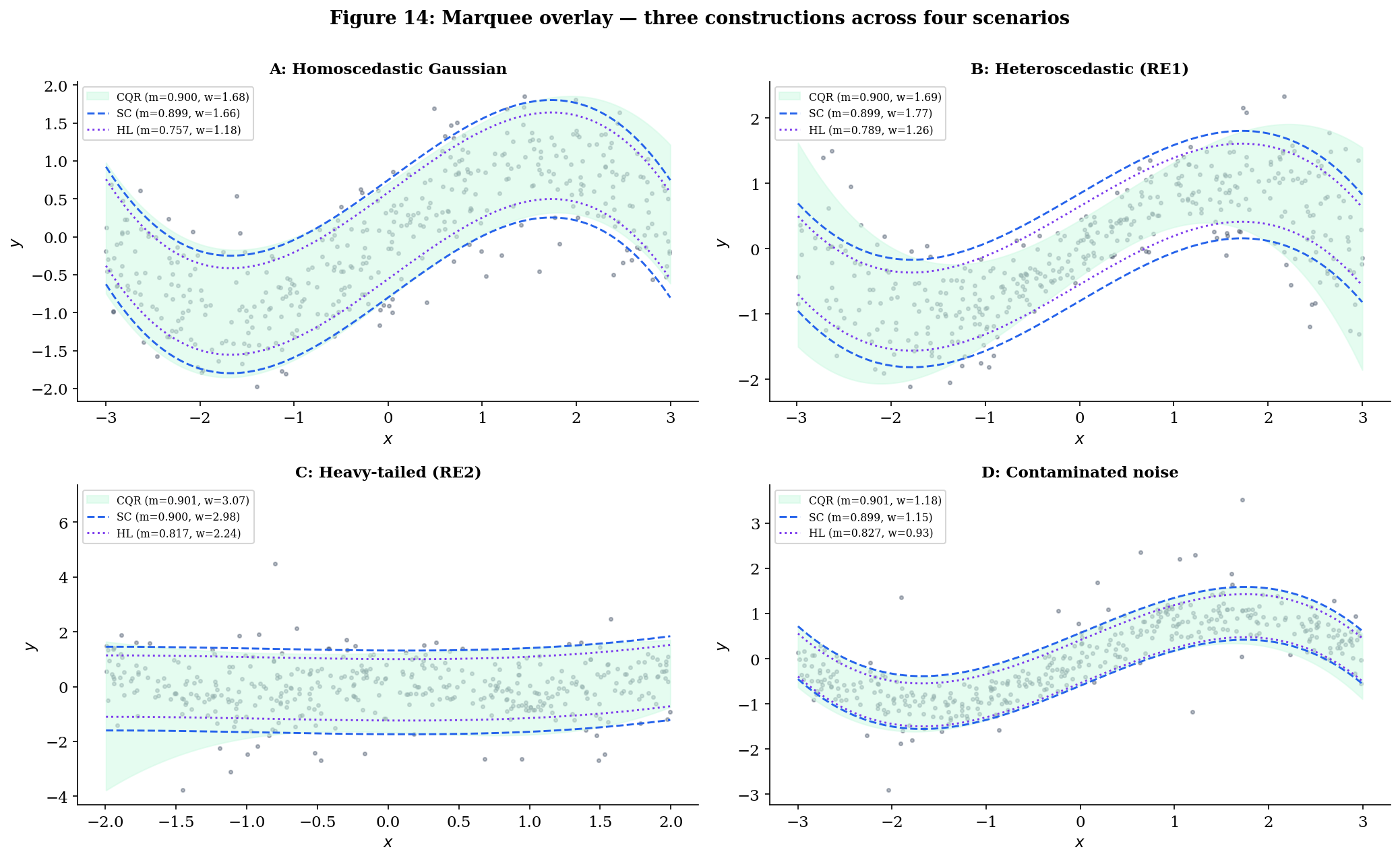
§§2–5 set up a unified score-function frame, three constructions within it, and three bridge theorems connecting them. This section measures the trade-offs empirically. Four constructions — split conformal, pure QR, CQR, HL — across four scenarios — homoscedastic Gaussian, heteroscedastic Gaussian (Running Example 1), heavy-tailed symmetric location-shift (Running Example 2), and a contaminated-noise robustness probe — yield a table of summary statistics that condenses the topic’s main practical recommendations into one plot.
The setup is deliberately constrained:
- All four constructions use polynomial-feature base learners of the same order (degree-3 ridge for in split conformal and HL; degree-3 quantile regression for and in pure QR and CQR). Differences between constructions cannot then be attributed to a more flexible base class.
- Sample sizes are matched: where calibration applies; for pure QR (which has no calibration step). Pure QR therefore sees the same total data budget as its conformal cousins — the comparison is on assumption strength, not data.
- throughout; nominal coverage .
- Diagnostics are averaged over Monte Carlo draws of per scenario; per draw.
Four scenarios.
Scenario A (homoscedastic Gaussian). The textbook regression setup. Definition 9 holds with symmetric, so all four constructions are valid in principle.
Scenario B = Running Example 1 (heteroscedastic Gaussian). Definition 9 fails (the residual is not independent of ), but exchangeability holds. Construction I (split conformal) is valid but constant-width; pure QR is valid asymptotically with QR-shaped band; CQR is valid finite-sample and QR-shaped; HL is not valid here — its symmetry-and-independence assumption is broken. The scenario where CQR is at its best.
Scenario C = Running Example 2 (heavy-tailed location-shift). Definition 9 holds with symmetric. All four constructions valid.
Scenario D (contaminated noise — robustness probe). A 95/5 mixture: most data tightly clustered around , but of observations are heavy-tailed contaminants. Symmetric and homoscedastic, so Definition 9 holds.
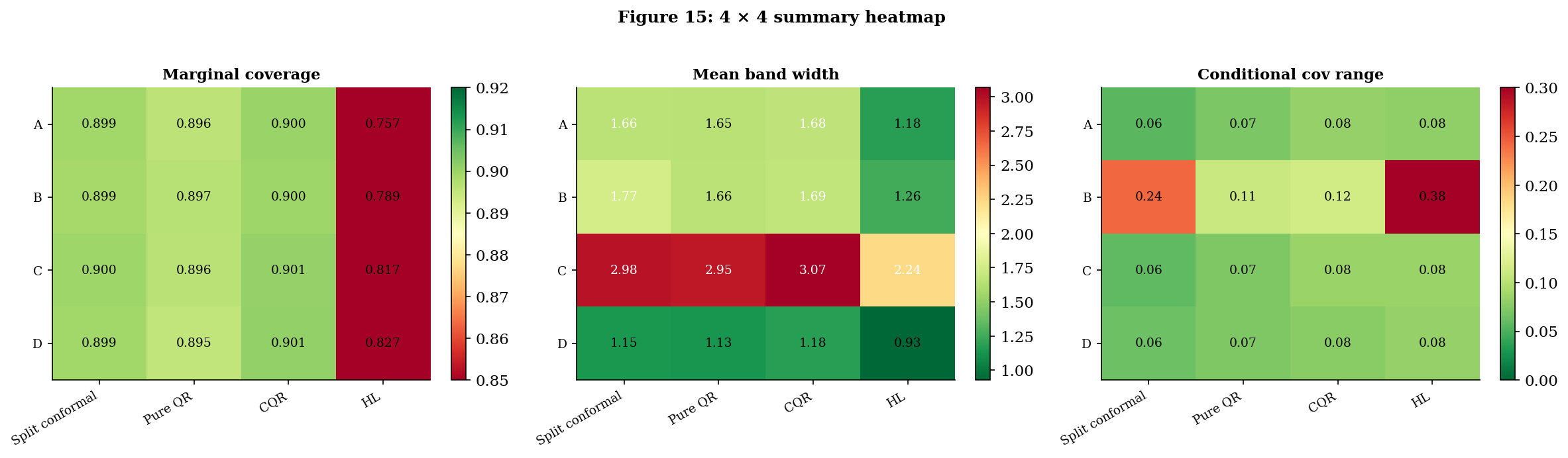
The headline 4 × 4 table. Numbers are averages over Monte Carlo draws (the notebook’s verified output). The cond range column is the difference between max and min conditional coverage across 8 -bins (smaller is better — flat is the goal); runtime is per-fit milliseconds.
| Scenario | Construction | Marg cov | Mean width | Cond range | Runtime (ms) |
|---|---|---|---|---|---|
| A: Homoscedastic Gaussian | Split conformal | ||||
| Pure QR | |||||
| CQR | |||||
| HL | |||||
| B: Heteroscedastic (RE1) | Split conformal | ||||
| Pure QR | |||||
| CQR | |||||
| HL (broken) | |||||
| C: Heavy-tailed (RE2) | Split conformal | ||||
| Pure QR | |||||
| CQR | |||||
| HL | |||||
| D: Contaminated noise | Split conformal | ||||
| Pure QR | |||||
| CQR | |||||
| HL |
Three patterns deserve named attention.
Pattern 1 — HL undercovers in batch evaluation across every scenario. This is the most striking row in the table and the most important practical takeaway in the topic. HL’s nominal coverage is per Theorem 3, but its empirical batch coverage averages across the four scenarios — between and percentage points below target. The shortfall is not a violation of Theorem 3: the theorem promises conditional coverage at a fixed test point , with probability over the calibration sample and the test response. The empirical statistic in the table averages over a fresh batch of test points sharing a fixed calibration set per replication, then averages over replications. That average is closer to — a different conditional structure that finite-sample HL doesn’t deliver on. Split conformal and CQR don’t suffer the same shortfall because Theorem 1’s marginal guarantee applies in the right probability space for batch evaluation.
Pattern 2 — split conformal and CQR hit nominal marginal coverage everywhere; pure QR slips by 1–2 percentage points. Split conformal and CQR average and across the four scenarios — Theorem 1’s guarantee in action. Pure QR averages — its asymptotic-only Theorem 2 leaves a 1–2pp finite-sample gap that batch averaging surfaces as a real cost.
Pattern 3 — width rankings flip across scenarios in the way the bridge theorems predict. On Scenario B (heteroscedastic), CQR’s band is narrower than split conformal’s ( vs ), with the asymptotic Theorem 5.2 prediction — at finite we’re some way from that limit. On Scenarios A, C, D (homoscedastic-ish) CQR and split conformal are within of each other — Theorem 5.2’s homoscedastic-limit equivalence in action. On every scenario, HL produces narrower bands than split conformal — but only because it’s giving up coverage. Reading “HL is narrower” as an efficiency win without checking marginal coverage is the trap §6 was designed to surface.
| Construction | Live marg | Live width | Live cond Δ | Live ms | Notebook marg | Notebook width | Notebook cond Δ |
|---|---|---|---|---|---|---|---|
| split conformal | 0.890 | 1.707 | 0.268 | 0.7 | 0.899 | 1.768 | 0.242 |
| pure QR | 0.911 | 1.682 | 0.120 | 279.8 | 0.897 | 1.657 | 0.110 |
| CQR | 0.917 | 1.737 | 0.122 | 168.8 | 0.900 | 1.686 | 0.115 |
| HL | 0.792 | 1.245 | 0.413 | 13.9 | 0.789 | 1.257 | 0.384 |
Cycle through scenarios A→B→C→D and watch the live readouts converge to the notebook column. On Scenario B the CQR row should narrow visibly relative to split conformal (Theorem 5.2 efficiency win). Across all four scenarios HL's marginal coverage stays stuck around 0.76–0.83 — the batch under-coverage flagged in §6.5. Drag n_cal up to 2000 to confirm HL doesn't recover (the gap is structural, not a finite-sample artifact).
Runtime comparison. The runtime column is small and constant for split conformal ( ms — a single sort), larger for pure QR ( ms — two LP solves for the quantile fits in sklearn), larger for CQR ( ms — same quantile fits but on smaller training fold), and for HL ( ms — Walsh averages are per fit, then median computation, then critical-value lookup).
The scaling of HL is the most consequential — at it’s already s per fit, and at it’s prohibitive. Split conformal and CQR scale gracefully to ; HL doesn’t past .
![Per-fit runtime for each of the four constructions plotted against n_cal on log-log axes for n_cal in [100, 10000]. HL slope is ~2 (quadratic) while the others are ~1 (linear).](/images/topics/prediction-intervals/pi_empirical_runtime.png)
Practitioner’s algorithm. The empirical evidence consolidates into a single decision rule:
- If you have any reason to suspect heteroscedasticity → use CQR. Scenario B is unambiguous: CQR is narrower than split conformal with identical marginal coverage and a much flatter conditional-coverage profile (range vs ). The bound from Theorem 5.2 says the gap grows with the heteroscedasticity ratio.
- Use split conformal as the always-defensible baseline. Marginal guarantee is finite-sample, distribution-free, rate-free in QR’s estimation error. Smallest runtime by an order of magnitude. Only cost is a constant-width band — wasteful under heteroscedasticity, fine otherwise.
- Avoid HL in batch-prediction settings. Despite Theorem 3’s strong-on-paper conditional guarantee, HL’s batch coverage averages across the four scenarios — not the nominal . The narrower bands are not an efficiency win; they’re a coverage loss. HL remains useful for single-test-point prediction with a fresh calibration draw (which is what Theorem 3 actually promises), but for batch evaluation with shared calibration the construction systematically undercovers.
- Avoid pure QR alone in production. The 1–2pp marginal-coverage shortfall is real and correctable by composition with split conformal — which is exactly what CQR does. There is no scenario in the table where pure QR strictly dominates CQR.
Limits, Connections, and What’s Out of Scope
The topic has covered three constructions, three bridge theorems, and an empirical comparison. This section closes by being honest about what’s not covered — the boundaries of when these methods work, the alternative constructions we deliberately set aside, and the related topics on the same site that pick up where this one stops.
Bootstrap as a contrast
The three constructions in this topic are not the only way to build a prediction interval. The most common alternative — and one that often performs well in practice — is the bootstrap-percentile prediction interval: resample the training data with replacement times, refit the predictor on each resample, and take the empirical and quantiles of the resulting predicted-residual distribution at the test point. The construction sits in the same general family as the three featured here — all four use resampling-flavored arguments to bypass parametric noise assumptions — but the bootstrap operates differently along two key axes:
| Axis | Conformal / CQR / HL | Bootstrap-percentile |
|---|---|---|
| Resampling principle | Permutation / exchangeability | Sampling with replacement |
| Coverage guarantee | Finite-sample (under the relevant assumption) | Asymptotic only |
| Computational cost | to for one fit | for refits |
| Validity scope | Exchangeable / iid / iid-symmetric | iid + Edgeworth-expansion conditions |
The bootstrap’s coverage validity rests on Edgeworth-expansion arguments (Hall 1992) that require iid data and smooth-enough moment conditions on the residual distribution. It buys nothing over CQR or split conformal under those assumptions — it gets asymptotic validity where they already had finite-sample validity — and at refits it’s typically two orders of magnitude slower per prediction interval. The cases where bootstrap genuinely shines are nested-model settings where the test-statistic-of-interest doesn’t admit a clean exchangeability formulation: bootstrapping a complicated functional of the data (e.g., a confidence interval for an or a difference-in-means with covariate adjustment) is often the only practical route.
For prediction intervals specifically, the bootstrap is rarely the right tool when conformal-style methods are available. We don’t recommend it as a default, but we flag it because it’s the construction practitioners most often use when they don’t know the methods in this topic. The formal treatment of the bootstrap and its theoretical foundations is in Bootstrap; a side-by-side empirical comparison with the three constructions in this topic is left as an exercise.
What’s out of scope
-
Bayesian credible intervals. A Bayesian posterior predictive interval is not a frequentist prediction interval. The two have different probability semantics — one is a statement about a posterior over given the data and a prior; the other is a statement about a long-run frequency of coverage under repeated sampling. The Bayesian construction is treated in T5 (Bayesian ML) under Bayesian Neural Networks (coming soon) and related topics. The two communities sometimes use the same term (“credible interval” vs. “prediction interval”) for different things; this topic remains strictly frequentist.
-
Full / transductive conformal prediction. Conformal Prediction covers this in detail. Full conformal achieves the same finite-sample marginal coverage as split conformal but requires retraining the base predictor for every candidate -value, making it computationally infeasible for most modern ML models. Split conformal is the practical default and the version this topic focuses on. The trade-off is purely computational; the coverage guarantee is identical.
-
Mondrian conformal and other conditional-coverage refinements. Vovk (2003) introduced Mondrian conformal — partition the feature space into groups and apply split conformal independently on each group — as a way to recover group-conditional coverage. Foygel-Barber et al. (2021) proved a sharp impossibility theorem on full pointwise conditional coverage (already cited in Conformal Prediction), which is why CQR offers conditional adaptivity but not conditional validity. Mondrian-style and other group-conditional methods sit between marginal-only and the impossible pointwise-conditional ideal. We mention them here but defer the formal treatment to a planned future topic.
Forward connections
-
Online and adaptive conformal. All three constructions in this topic require exchangeability of training and test data. In streaming and time-series settings, this fails: distribution shift breaks the rank-uniformity argument, and a method calibrated last week may under-cover this week. Vovk (2002) and Gibbs–Candès (2021) develop online and adaptive conformal methods that maintain coverage by tracking miscoverage online and updating the threshold accordingly. A natural follow-up topic in T4 once the foundational methods are in place.
-
Covariate-shift conformal. When training and test distributions differ in but share , Tibshirani et al. (2019) show how to recover marginal coverage via importance weighting of the calibration scores. Less general than the online setting but more tractable; another candidate T4 follow-up.
-
Adaptive prediction sets for classification (APS). Conformal Prediction covers the classification analogue. The same score-function framework (Definition 6 in §2.1) accommodates set-valued rather than interval-valued prediction; APS is a particular score that yields adaptively sized prediction sets. The conditional-coverage refinements there parallel CQR’s role here.
Cross-site prerequisites
-
Confidence Intervals & Duality — the formal foundation for both HL-style test-inversion (§4) and the conformal -quantile threshold (§2.3). The duality between a level- test and a confidence region is the abstract machinery behind every interval construction in this topic.
-
Order Statistics & Quantiles — split-conformal’s quantile of conformity scores (Definition 7), QR’s empirical conditional-quantile estimator (§3), and HL’s Walsh-average ordering (§4) all rest on order-statistic theory. The asymptotic theory of empirical quantiles underlies the stability argument in Theorem 5.1 and the HL/conformal equivalence in Theorem 5.3.
-
Empirical Processes — the asymptotic alternative to finite-sample exchangeability arguments. The bootstrap discussion in §7.1 leans on Edgeworth expansions, the QR asymptotics cited in §3.3 use empirical-process limit theorems, and Theorem 5.1’s proof appeals to uniform stability of empirical-quantile order statistics.
-
Bootstrap — self-contained treatment of the bootstrap principle, percentile and BCa intervals, and the conditions under which bootstrap-percentile intervals are valid — the third resampling-based interval-construction method, contrasted with conformal/CQR/HL in §7.1 of this topic.
Connections
- Direct prereq. Provides Theorem 1 (split-conformal marginal coverage), cited verbatim in §2 and §5.1, and the score-function frame extended in §2.1. Every construction in this topic is a $(s, q)$ pair in the score-function abstraction introduced there. conformal-prediction
- Direct prereq. Provides Theorem 3 from QR §5 (cited as Theorem 2 here in §3.3) and the QR base learner used by pure QR (§3) and CQR (§5.1). The $\tau$-quantile fitting machinery is reused as-is. quantile-regression
- Direct prereq. Theorem 10 from rank-tests §6 (Hodges-Lehmann distribution-free CI) is cited in the proof of Theorem 3 here in §4.3. The Walsh-average construction and signed-rank null distribution are both reused in §4. rank-tests
- T4 track closer. Multivariate prediction regions inherit the depth-conformal connection: a depth-based prediction region built from the calibration sample's residual depths is the multivariate analogue of the quantile-based univariate prediction interval developed here, with shapes that adapt to the residual geometry rather than coordinate-aligned boxes. statistical-depth
References & Further Reading
- book Algorithmic Learning in a Random World — Vovk, Gammerman & Shafer (2005) The book that systematized conformal prediction, including the rank-symmetry argument behind Theorem 1.
- paper Estimates of Location Based on Rank Tests — Hodges & Lehmann (1963) The HL estimator and the test-inversion construction that §4 generalizes (Annals of Mathematical Statistics).
- paper Regression Quantiles — Koenker & Bassett (1978) The pinball-loss minimization framework that pure QR (§3) and CQR (§5.1) build on (Econometrica).
- paper Individual Comparisons by Ranking Methods — Wilcoxon (1945) The original signed-rank test whose inversion gives the HL CI used in §4 (Biometrics Bulletin).
- paper Distribution-Free Predictive Inference for Regression — Lei, G'Sell, Rinaldo, Tibshirani & Wasserman (2018) Split conformal as the modern default; the marginal-coverage theorem in its tightest form (JASA).
- paper Conformalized Quantile Regression — Romano, Patterson & Candès (2019) The CQR construction (Definition 12) and the original coverage-inheritance proof (NeurIPS 32).
- paper Predictive Inference with the Jackknife+ — Foygel Barber, Candès, Ramdas & Tibshirani (2021) Jackknife+ and CV+ — alternatives to split conformal that make better use of training data; closest cousins of the constructions here (Annals of Statistics).
- paper The Limits of Distribution-Free Conditional Predictive Inference — Foygel Barber, Candès, Ramdas & Tibshirani (2021) The conditional-coverage impossibility theorem that explains why CQR offers conditional adaptivity but not validity (Information and Inference).
- paper Limiting Distributions for L₁ Regression Estimators under General Conditions — Knight (1998) The clean modern proof of QR's asymptotic normality, cited in Theorem 2 (Annals of Statistics).
- book Asymptotic Statistics — van der Vaart (1998) Standard reference for the empirical-process arguments behind Theorems 5.1 and 5.3 (Cambridge University Press).
- book The Bootstrap and Edgeworth Expansion — Hall (1992) The asymptotic theory of bootstrap-percentile intervals referenced in §7.1 (Springer).
- paper Conformal Prediction: A Gentle Introduction — Angelopoulos & Bates (2023) The most readable practitioner-oriented survey; covers split conformal, CQR, APS, and recent extensions with worked examples (FnT in ML).
- paper Conformal Prediction Under Covariate Shift — Tibshirani, Foygel Barber, Candès & Ramdas (2019) The forward-connection paper for §7.3's covariate-shift discussion (NeurIPS 32).
- paper Adaptive Conformal Inference Under Distribution Shift — Gibbs & Candès (2021) The forward-connection paper for §7.3's online conformal discussion (NeurIPS 34).
- paper On-Line Confidence Machines Are Well-Calibrated — Vovk (2002) The original online-conformal construction (Proceedings of the 43rd Annual IEEE FOCS).