Conformal Prediction

Distribution-Free Prediction and the Exchangeability Setup

We observe $n$ feature–response pairs $(X_1, Y_1), \ldots, (X_n, Y_n)$ and want to say something useful about the next pair $(X_{n+1}, Y_{n+1})$ . A point estimate $\hat\mu(X_{n+1})$ answers “what’s the most likely value of $Y_{n+1}$ ” but leaves “how much should we trust this answer” untouched. A prediction set $\hat C_\alpha(X_{n+1}) \subseteq \mathcal{Y}$ is a data-dependent subset of the response space chosen so that

\mathbb{P}\bigl( Y_{n+1} \in \hat C_\alpha(X_{n+1}) \bigr) \;\geq\; 1 - \alpha,

where $\alpha \in (0, 1)$ is the miscoverage level and the probability is over the joint distribution of training, calibration, and test data. Conformal prediction is the construction that makes $\hat C_\alpha$ valid in this sense — without distributional assumptions on $(X, Y)$ , without bounded-noise hypotheses, and without asymptotics. The only assumption is exchangeability.

Two structural points distinguish a prediction set from a confidence interval. First, a confidence interval covers a fixed parameter (a population mean, a quantile $\xi_p$ ); a prediction set covers a random variable — the unobserved $Y_{n+1}$ . Second, the confidence interval shrinks at rate $1/\sqrt{n}$ as the sample size grows, whereas the prediction set has an irreducible width set by the noise distribution: even with infinite training data, a prediction set for $Y_{n+1} \mid X_{n+1}$ can never be tighter than the conditional spread of $Y$ at that input.

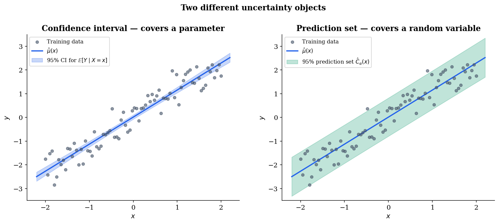
Side-by-side panels showing a confidence band for the conditional mean (narrow, shrinks with n) and a prediction set for the next observation (wider, set by noise scale) — Confidence intervals shrink at rate 1/√n and cover the regression function E[Y | X = x]. Prediction sets accommodate the irreducible noise of Y | X and have a width floor independent of n. The two objects answer different questions.

This contrast — CI for a parameter, prediction set for a random variable — is the same one that formalStatistics: Order Statistics & Quantiles draws when introducing distribution-free CIs for the population quantile $\xi_p$ via paired order statistics. The argument used there relies on rank symmetry under exchangeability, and Topic 29 §29.10 Remark 21 explicitly motivates Vovk–Gammerman–Shafer’s distribution-free prediction as the natural generalization from a fixed parameter to a random variable. We will see this same rank-symmetry machinery in §3’s proof of marginal coverage.

Definition 1 (Exchangeability).

A finite sequence of random variables $Z_1, \ldots, Z_N$ is exchangeable if its joint distribution is invariant under coordinate permutation: for every permutation $\pi$ of $\{1, \ldots, N\}$ ,

(Z_1, \ldots, Z_N) \;\stackrel{d}{=}\; (Z_{\pi(1)}, \ldots, Z_{\pi(N)}).

Exchangeability is strictly weaker than iid. Every iid sample is exchangeable — permuting independent draws from a common distribution leaves the joint law unchanged — but the converse fails: an urn drawn without replacement is exchangeable (any permutation of the draws is equally likely as a sequence) yet not iid (later draws depend on earlier ones). The structure of exchangeable sequences is described by de Finetti’s representation theorem: an infinite exchangeable sequence is a mixture of iid sequences, with the mixing measure capturing whatever shared latent structure links the observations. For finite-sample purposes, that subtlety doesn’t bite — what we need is the symmetry property itself.

The bet conformal prediction makes is that exchangeability holds for the augmented sequence $(X_1, Y_1), \ldots, (X_{n+1}, Y_{n+1})$ — training, calibration, and test points all drawn from the same source. This is genuinely weaker than iid: it accommodates dependence within the dataset (the urn case, time-series with stationary increments, certain sampling-without-replacement designs) provided that no observation has a privileged position. What it does not accommodate is distribution shift — a test distribution that differs from the training distribution. We return to this in §8, where we visualize how naive conformal prediction degrades under covariate shift and see how the importance-weighted variant of formalStatistics: Empirical Processes ‘s sister technique (Tibshirani et al. 2019) restores marginal coverage when the shift is known.

The asymptotic alternative to conformal prediction is the empirical-processes route: Topic 32 of formalstatistics develops uniform-convergence bounds (DKW, VC dimension, Glivenko–Cantelli) that imply distribution-free coverage in the large- $n$ limit. Conformal prediction sidesteps the uniform-convergence rate entirely — it gives an exact finite-sample statement — at the price that the coverage is marginal rather than conditional (a distinction that becomes the impossibility theorem of §8). Both routes lead to distribution-free prediction; they pay different prices.

Split (Inductive) Conformal Prediction

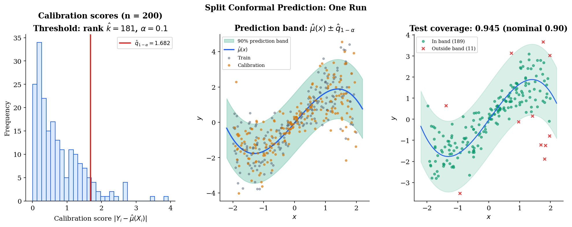
The simplest realization of the marginal-coverage promise — and the one used in essentially every modern application — is split conformal prediction, sometimes called inductive conformal prediction. The construction is mechanical: split the data into a training set and a calibration set, fit a predictor on the former, score residuals on the latter, take an empirical quantile, declare the prediction interval. Three short paragraphs and a definition cover everything; the depth is in the proof, which lands in §3.

Partition the $n$ available observations into a training set of size $m$ and a calibration set of size $n_{\text{cal}}$ :

\underbrace{(X_1, Y_1), \ldots, (X_m, Y_m)}_{\text{training}} \quad\text{and}\quad \underbrace{(X_{m+1}, Y_{m+1}), \ldots, (X_{m+n_{\text{cal}}}, Y_{m+n_{\text{cal}}})}_{\text{calibration}}.

Then run four steps.

Step 1 — Fit. Train a base predictor $\hat\mu$ using only the training set. The base predictor can be anything — ridge regression, a random forest, a neural network — and the coverage guarantee will not depend on what it is. The quality of $\hat\mu$ controls the width of the prediction interval, not its validity.

Step 2 — Score. Compute a nonconformity score $S_i = s(X_i, Y_i)$ at each calibration point. For regression, the standard choice is the absolute residual $S_i = |Y_i - \hat\mu(X_i)|$ ; for classification we will use a different score in §7. The score is “large when $(X, Y)$ looks anomalous given the fitted model.”

Step 3 — Threshold. Take the $\hat k = \lceil (1 - \alpha)(n_{\text{cal}} + 1) \rceil$ -th smallest calibration score and call this value $\hat q_{1-\alpha}$ . (When $\hat k > n_{\text{cal}}$ — which happens for very small calibration sets — cap at $n_{\text{cal}}$ , equivalently set $\hat q_{1-\alpha} = +\infty$ and the interval becomes all of $\mathbb{R}$ .)

Step 4 — Predict. For a new test point $X_{n+1}$ , the prediction set is the level- $\hat q_{1-\alpha}$ sublevel set of the score:

\hat C_\alpha(X_{n+1}) \;=\; \bigl\{ y \in \mathcal{Y} \,:\, s(X_{n+1}, y) \le \hat q_{1-\alpha} \bigr\}.

For the absolute-residual score this resolves to a symmetric interval centered on the prediction, $[\hat\mu(X_{n+1}) - \hat q_{1-\alpha},\ \hat\mu(X_{n+1}) + \hat q_{1-\alpha}]$ . The interval has the same half-width $\hat q_{1-\alpha}$ at every test point, regardless of $X_{n+1}$ — split conformal with this score is not locally adaptive. We address that in §6 (CQR).

Definition 2 (Split Conformal Prediction Set).

With training-fitted predictor $\hat\mu$ , calibration set of size $n_{\text{cal}}$ , nonconformity score $s$ , and miscoverage level $\alpha \in (0, 1)$ , the split conformal prediction set at input $x$ is

\hat C_\alpha(x) \;=\; \bigl\{ y \in \mathcal{Y} \,:\, s(x, y) \le \hat q_{1-\alpha} \bigr\},

where $\hat q_{1-\alpha}$ is the

\hat k \;=\; \bigl\lceil (1 - \alpha)(n_{\text{cal}} + 1) \bigr\rceil

smallest of the calibration scores $(S_i)_{i=1}^{n_{\text{cal}}}$ .

The " $+1$ " inside the ceiling deserves a moment. It looks fussy — and it is, in the sense that for moderate $n_{\text{cal}}$ it changes $\hat q_{1-\alpha}$ by at most one rank — but it is also load-bearing. Under exchangeability, the (unobserved) test-point score $S_{n+1}$ will be inserted into the augmented sequence $(S_1, \ldots, S_{n_{\text{cal}}+1})$ at a uniformly random rank in $\{1, \ldots, n_{\text{cal}} + 1\}$ . The ceiling-and-plus-one converts that rank uniformity directly into the marginal-coverage probability. Drop the $+1$ and the bound is no longer tight; replace the ceiling with a floor and the bound flips to a strict inequality in the wrong direction. We reconstruct this argument in §3.

Three-panel figure showing one run of split conformal: histogram of calibration scores with the threshold line, prediction band overlaid on training and calibration data, and a test set colored by whether each observation falls inside the band — One run of split conformal on heteroscedastic regression data. Left: calibration scores (absolute residuals between observed and predicted y) with the rank-181 threshold at α = 0.10, n_cal = 200. Middle: the symmetric prediction band (predictor ± threshold) — note the constant width independent of x. Right: empirical coverage on a held-out test set (90.0% here, against a target of 90%). The width insensitivity to x is what CQR (§6) fixes.

The construction is so spare that it raises an immediate question: why does this work? Nothing in steps 1–4 used the joint distribution of $(X, Y)$ , the smoothness of $\hat\mu$ , or any property of the base predictor beyond its having been fit before the calibration scores were computed. The next section gives the answer — Theorem 1 (marginal coverage), proved entirely from rank symmetry under exchangeability.

Marginal Coverage: The Central Theorem

Theorem 1 is the reason split conformal works. It is also the reason the construction is so insensitive to the choice of base predictor and nonconformity score — the proof never opens those black boxes. Everything follows from a single combinatorial fact: under exchangeability, the test-point score is equally likely to land at any rank within the augmented sequence of calibration-plus-test scores. Convert that rank uniformity to a coverage probability, and the bound is finite-sample, two-sided, and tight.

Theorem 1 (Marginal Coverage — Lei, G'Sell, Rinaldo, Tibshirani & Wasserman 2018).

Let $(X_i, Y_i)_{i=1}^{n_{\text{cal}} + 1}$ be exchangeable, where the first $n_{\text{cal}}$ pairs constitute the calibration set and $(X_{n_{\text{cal}}+1}, Y_{n_{\text{cal}}+1})$ is a test point. Suppose the nonconformity score $s$ does not depend on the calibration or test set — for example, it depends only on a separately-trained predictor. Then the split conformal prediction set $\hat C_\alpha$ at level $\alpha \in (0, 1)$ satisfies

\mathbb{P}\bigl( Y_{n_{\text{cal}}+1} \in \hat C_\alpha(X_{n_{\text{cal}}+1}) \bigr) \;\geq\; 1 - \alpha.

Moreover, if the score distribution is continuous (no ties almost surely),

\mathbb{P}\bigl( Y_{n_{\text{cal}}+1} \in \hat C_\alpha(X_{n_{\text{cal}}+1}) \bigr) \;\leq\; 1 - \alpha + \frac{1}{n_{\text{cal}} + 1}.

Proof.

Let $S_i = s(X_i, Y_i)$ for $i = 1, \ldots, n_{\text{cal}} + 1$ . Because $s$ is a fixed function — the training set has been consumed already, and $s$ does not depend on the remaining $n_{\text{cal}} + 1$ points — exchangeability of the underlying pairs lifts to exchangeability of the scores: the joint distribution of $(S_1, \ldots, S_{n_{\text{cal}}+1})$ is invariant under any permutation of indices.

Let $R$ denote the rank of the test-point score $S_{n_{\text{cal}}+1}$ in the augmented vector $(S_1, \ldots, S_{n_{\text{cal}}+1})$ , that is,

R \;=\; \#\bigl\{ i \in \{1, \ldots, n_{\text{cal}} + 1\} \,:\, S_i \le S_{n_{\text{cal}}+1} \bigr\}.

Continuity of the score distribution ensures no ties almost surely, so $R$ is well-defined as an integer in $\{1, \ldots, n_{\text{cal}} + 1\}$ . Exchangeability means each of the $n_{\text{cal}} + 1$ positions is equally likely to be the test point’s, so

\mathbb{P}(R = j) \;=\; \frac{1}{n_{\text{cal}} + 1} \quad \text{for each } j \in \{1, \ldots, n_{\text{cal}} + 1\}. \tag{$\ast$}

In words: $R$ is uniformly distributed on $\{1, \ldots, n_{\text{cal}} + 1\}$ . This is the only probabilistic fact the proof needs.

Set $\hat k = \lceil (1 - \alpha)(n_{\text{cal}} + 1) \rceil$ . The prediction set covers $Y_{n_{\text{cal}}+1}$ iff the test score lies at or below the threshold:

\begin{aligned} Y_{n_{\text{cal}}+1} \in \hat C_\alpha \;&\iff\; S_{n_{\text{cal}}+1} \le \hat q_{1-\alpha} \\ \;&\iff\; S_{n_{\text{cal}}+1} \text{ ranks at most } \hat k \text{ among } (S_1, \ldots, S_{n_{\text{cal}}}). \end{aligned}

A short combinatorial step converts the calibration-set rank to the augmented-set rank. If $S_{n_{\text{cal}}+1}$ occupies augmented rank $R$ , exactly $R - 1$ of the augmented scores are strictly smaller than it; each of those $R - 1$ smaller scores must lie in the calibration set (the test set contributes only $S_{n_{\text{cal}}+1}$ itself). So $S_{n_{\text{cal}}+1}$ ranks at most $\hat k$ among the calibration scores precisely when $R \le \hat k$ :

S_{n_{\text{cal}}+1} \text{ ranks at most } \hat k \text{ among calibration scores} \;\iff\; R \le \hat k.

Combining with ( $\ast$ ):

\mathbb{P}\bigl( Y_{n_{\text{cal}}+1} \in \hat C_\alpha \bigr) \;=\; \mathbb{P}(R \le \hat k) \;=\; \frac{\hat k}{n_{\text{cal}} + 1}.

The lower bound is immediate from the definition of $\hat k$ :

\hat k \;=\; \lceil (1 - \alpha)(n_{\text{cal}} + 1) \rceil \;\geq\; (1 - \alpha)(n_{\text{cal}} + 1),

so $\mathbb{P}(Y_{n_{\text{cal}}+1} \in \hat C_\alpha) \ge 1 - \alpha$ . For the upper bound, use $\lceil z \rceil \le z + 1$ :

\hat k \;\leq\; (1 - \alpha)(n_{\text{cal}} + 1) + 1,

\mathbb{P}\bigl( Y_{n_{\text{cal}}+1} \in \hat C_\alpha \bigr) \;\leq\; (1 - \alpha) + \frac{1}{n_{\text{cal}} + 1}.

∎

Remark (Marginal Coverage Proof Independence).

The proof never opens the black box of $\hat\mu$ or invokes a property of the data beyond exchangeability. It does not assume that $Y$ has finite moments, that $X$ lies in a bounded set, or that the marginal distribution is continuous — only that the score distribution is continuous (which holds almost surely whenever $Y \mid X$ has a continuous conditional density, the typical regression setting). The score function $s$ is chosen by the analyst; the only restriction is that $s$ not depend on the calibration or test data, equivalent to fitting any tunable parts of $s$ — including the predictor $\hat\mu$ and its hyperparameters — using only the training set.

The two-sided bound says coverage concentrates in a strip of width $\frac{1}{n_{\text{cal}} + 1}$ above $1 - \alpha$ . At $n_{\text{cal}} = 200$ and $\alpha = 0.10$ the strip is $[0.90,\ 0.9050]$ — only $0.5$ percentage points wide. The next visualization runs $T = 500$ Monte Carlo trials at user-controlled $(\alpha, n_{\text{cal}})$ and shows the empirical coverage histogram concentrating inside the predicted band. Drag the calibration-size slider to see the strip narrow as $n_{\text{cal}}$ grows — and notice that even the $n_{\text{cal}} = 20$ regime (where the upper bound is fully $5$ percentage points above $1 - \alpha$ ) preserves marginal validity in expectation.

α0.10n_calT = 500 trials · n_train = 300 · n_test/trial = 20

Drag α to retarget coverage; switch n_cal to see the upper-bound strip narrow as 1/(n_cal+1) shrinks. The middle-panel histogram concentrates inside the orange [1−α, 1−α+1/(n_cal+1)] band predicted by Theorem 1; the bottom-panel running mean converges into the same band as t → T. The top panel's red test points are the rare misses (~α fraction).

Four-panel verification: running coverage convergence over T trials, coverage stability across calibration-set sizes, coverage as a function of alpha, and distribution of batched coverage values relative to the theoretical bounds

Empirical confirmation across configurations: split conformal coverage stays inside the [1−α, 1−α + 1/(n_cal + 1)] band predicted by Theorem 1. The bottom-right panel chunks T = 4000 trials into batches of 100 and plots the per-batch coverage against the lower-bound (red dashed) and upper-bound (amber dotted) lines — the bounds are demonstrably tight, not loose.

The bound is tight, not just a one-sided guarantee — and that tightness is doing real work. A naive reading of " $\ge 1 - \alpha$ " might suggest the procedure could over-cover wildly with no statistical penalty, but Theorem 1’s upper bound rules that out: split conformal does not waste coverage. As long as the score distribution is continuous and exchangeability holds, the procedure delivers within $\tfrac{1}{n_{\text{cal}} + 1}$ of nominal — no looser, no tighter.

What the bound does not say is anything about conditional coverage at a specific $X = x$ . The marginal probability averages over the distribution of $X$ , so a procedure that under-covers in one region and over-covers in another can still satisfy Theorem 1. We return to this in §8 with the Foygel-Barber 2021 impossibility theorem.

Cross-Validation in Conformal: CV+

Split conformal pays a calibration tax. The data partition $(m,\ n_{\text{cal}})$ has to allocate enough mass to the calibration set for the threshold to be stable — typically $n_{\text{cal}} \approx n/2$ — which means the predictor $\hat\mu$ trains on only half the available data. For a fixed total budget $n$ this is genuinely wasteful: a better $\hat\mu$ would mean tighter prediction intervals (recall, the width depends on predictor quality even though validity doesn’t).

Cross-validation offers a way out. Partition $\{1, \ldots, n\}$ into $K$ folds of roughly equal size, and for each fold $k$ fit a predictor $\hat\mu_{-k}$ on the data with fold $k$ removed. The leave-one-fold-out residual at observation $i$ is

R_i \;=\; \bigl| Y_i - \hat\mu_{-\text{fold}(i)}(X_i) \bigr|,

and the CV+ prediction interval uses these residuals — combined with per-fold predictions at the test point — through the same quantile construction we will introduce for jackknife+ in §5. Every observation contributes to both the fit and the residual scoring; no calibration tax.

The trade-off is computational. Jackknife+ ( $K = n$ ) requires $n$ predictor fits; $K$ -fold CV+ requires only $K$ fits, typically $K = 5$ or $K = 10$ . For expensive base predictors — random forests, neural networks, anything that costs minutes per fit — CV+ is the only practical route. The coverage guarantee is identical: Theorem 2 in §5 establishes the lower bound $\mathbb{P}(Y_{n+1} \in \hat C_\alpha^{\text{CV+}}) \ge 1 - 2\alpha$ for both jackknife+ ( $K = n$ ) and $K$ -fold CV+ verbatim. The factor of $2$ is worst-case over base predictors; in practice, both procedures achieve coverage very close to nominal $1 - \alpha$ .

The full procedural definition, the BCRT 2021 tournament/comparison-graph proof, and the empirical comparison to split conformal all live in §5. The anchor here exists so that any sister-site reference to “cross-validation in machine learning” can deep-link to a coherent treatment without minting a separate topic.

Full (Transductive) Conformal Prediction

CV+ avoids the calibration tax by recycling fits across folds. Full conformal — the original Vovk-Gammerman-Shafer construction — avoids it differently: by treating the candidate response itself as the variable and refitting the predictor once per candidate. Every observation is used for both fitting and calibration; the price is a per-candidate refit at test time.

The procedure. To form the prediction set $\hat C_\alpha(X_{n+1})$ at a new test input $X_{n+1}$ , iterate over candidate values $y \in \mathcal{Y}$ and for each one run four steps.

Step 1 — Augment. Form the augmented dataset $\mathcal{D}_y = \{(X_i, Y_i)\}_{i=1}^{n} \cup \{(X_{n+1}, y)\}$ — the original $n$ observations plus the test input paired with the candidate $y$ .

Step 2 — Fit. Fit a predictor $\hat\mu_y$ on $\mathcal{D}_y$ , or equivalently define a score function $s_y$ from $\mathcal{D}_y$ .

Step 3 — Score. Compute calibration scores $S_i^{(y)} = s_y(X_i, Y_i)$ for $i = 1, \ldots, n+1$ — every observation, including the augmented test pair.

Step 4 — Include. Include $y$ in $\hat C_\alpha(X_{n+1})$ iff the rank of $S_{n+1}^{(y)}$ among $(S_1^{(y)}, \ldots, S_{n+1}^{(y)})$ is at most $\lceil (1 - \alpha)(n + 1) \rceil$ .

The marginal-coverage guarantee extends from §3 with no change. When the candidate $y$ equals the true (unobserved) $Y_{n+1}$ , the augmented dataset is exchangeable, and Theorem 1’s argument — uniformity of the test-score rank in $\{1, \ldots, n+1\}$ — applies verbatim. Therefore $\mathbb{P}(Y_{n+1} \in \hat C_\alpha(X_{n+1})) \ge 1 - \alpha$ .

Why study it. Full conformal is rarely the practical default but it earns its keep on two counts. First, statistical efficiency: every observation contributes to both the fit and the rank computation, so for small $n$ — say $n \le 100$ — the prediction interval is meaningfully tighter than split conformal at the same $\alpha$ . Second, theoretical cleanliness: many extensions of conformal (online conformal under streaming data, conformal under model misspecification, conformal for transductive learning) are easier to state and analyze in the full-conformal framework, then specialized to split.

Computational cost. Naively, full conformal requires one predictor fit per candidate $y$ . For finite response spaces — classification with $K$ classes — this is $O(K)$ fits per test point, eminently tractable. For continuous regression, the candidate space must be discretized to a grid, giving $O(\text{grid size})$ fits, which gets expensive but is embarrassingly parallel. For specific predictors the per-candidate refit collapses: ridge regression admits closed-form leave-one-out updates that turn full conformal into a single $O(n)$ pass, and recent work has produced similar closed-form recipes for kernel ridge, lasso, and certain neural network families.

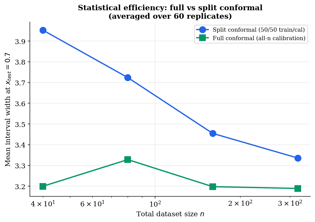
Line plot showing mean prediction interval width at a fixed test point as total dataset size n varies on a log scale, with split conformal (blue) consistently wider than full conformal (green), the gap closing as n grows — Statistical efficiency comparison at a fixed test location, averaged over 60 replicates. Split conformal (blue) splits 50/50 between train and calibration; full conformal (green) uses all n observations for both. The width gap is meaningful at small n (full is ~25% tighter at n = 40) and shrinks to noise as n → ∞. Split's calibration tax is real, but it's a tax on the small-data regime.

For most practical purposes — modern ML with $n$ in the thousands and base predictors that take seconds to fit — split conformal is the right default and the rest of this topic uses it. Full conformal sits in the toolkit for the small- $n$ regime, the closed-form-update predictors, and the theoretical extensions that are easier to derive there. Jackknife+ and CV+ in §5 carve out a middle ground: leave-one-out residuals through a small number of refits, with the same exchangeability machinery delivering a (slightly weaker) coverage bound.

Jackknife+ and CV+

Split conformal pays a calibration tax; full conformal pays a per-candidate refit tax. Jackknife+ (Foygel Barber, Candès, Ramdas & Tibshirani 2021) charts a third route: use every observation for both fitting and residual scoring through leave-one-out refitting. Each calibration residual is computed against a predictor that did not see that observation, restoring statistical efficiency without the per-candidate explosion of full conformal. The price is mild — $n$ predictor fits per training (one for each leave-one-out), parallelizable — and the coverage guarantee weakens by a factor of two.

For each $i \in \{1, \ldots, n\}$ , let $\hat\mu_{-i}$ denote the predictor fit on the dataset with the $i$ -th observation removed, and define the leave-one-out residual

R_i \;=\; \bigl| Y_i - \hat\mu_{-i}(X_i) \bigr|.

This $R_i$ is an honest residual in the sense that it never used $(X_i, Y_i)$ in its training — exactly the property split conformal extracted by partitioning the data, but achieved here without sacrificing any sample.

Definition 3 (Jackknife+ Prediction Interval).

The jackknife+ prediction interval at test point $X_{n+1}$ , miscoverage level $\alpha \in (0, 1)$ , is

\hat C_\alpha^{\text{J+}}(X_{n+1}) \;=\; \Bigl[\, \hat Q_\alpha^{-}\bigl\{ \hat\mu_{-i}(X_{n+1}) - R_i \bigr\},\ \hat Q_{1-\alpha}^{+}\bigl\{ \hat\mu_{-i}(X_{n+1}) + R_i \bigr\} \,\Bigr],

where $\hat Q_\alpha^{-}$ is the $\lfloor \alpha (n+1) \rfloor$ -th smallest of a collection of $n$ values (with $\hat Q_0^{-} = -\infty$ ) and $\hat Q_{1-\alpha}^{+}$ is the $\lceil (1-\alpha)(n+1) \rceil$ -th smallest (with $\hat Q_1^{+} = +\infty$ ).

The endpoints look more elaborate than the symmetric split-conformal interval, but each is just an empirical quantile of $n$ leave-one-out predictions adjusted by their respective residuals. The lower endpoint asks “across all leave-one-out fits, what’s the small-quantile of $\hat\mu_{-i}(X_{n+1}) - R_i$ ” — a low-side estimate that accommodates predictor variability across LOO fits and the residual magnitudes. The upper endpoint is symmetric. Crucially, the $i$ -th LOO predictor’s variability and its residual move together: a fold whose held-out point is hard to predict produces both a wild $\hat\mu_{-i}(X_{n+1})$ and a large $R_i$ , and the construction lets these self-correct.

Theorem 2 (Jackknife+ Coverage Bound — Foygel Barber, Candès, Ramdas & Tibshirani 2021).

Under exchangeability of $(X_i, Y_i)_{i=1}^{n+1}$ ,

\mathbb{P}\bigl( Y_{n+1} \in \hat C_\alpha^{\text{J+}}(X_{n+1}) \bigr) \;\geq\; 1 - 2\alpha.

The constant $2$ cannot be improved without further structural assumptions on the predictor: BCRT 2021 exhibit a degenerate base predictor under which jackknife+ achieves coverage arbitrarily close to $1 - 2\alpha$ .

Proof.

The proof follows BCRT 2021 §3.2; we reconstruct the key combinatorial moves and direct the reader to the original for the formalization of the tournament step.

For each $i \in \{1, \ldots, n\}$ , define the leave-one-out swap residual

R_i^{\ast} \;=\; \bigl| Y_{n+1} - \hat\mu_{-i}(X_{n+1}) \bigr|,

the absolute residual we would have observed if the test point $(X_{n+1}, Y_{n+1})$ had taken the role of training point $i$ and $(X_i, Y_i)$ had taken the role of the test point. By exchangeability of the $n+1$ observations together with the fact that the predictor $\hat\mu_{-i}$ is a symmetric function of its inputs (the order of the training observations does not matter), the joint distribution of the residuals is invariant under any swap of indices $(i, n+1)$ . In particular, $R_i$ and $R_i^{\ast}$ have the same marginal distribution for each $i$ .

Consider the comparison graph $G$ on vertex set $\{1, \ldots, n+1\}$ defined by placing a directed edge $i \to j$ whenever the leave- $\{i,j\}$ -out residual at $i$ exceeds the leave- $\{i,j\}$ -out residual at $j$ (BCRT 2021 §3.2). For the swap-symmetry argument, what matters is the pairwise comparison between each training index $i \in \{1, \ldots, n\}$ and the test index $n+1$ . The exchangeability swap above shows the comparison is symmetric in $i \leftrightarrow n+1$ , so the directed in-degree of vertex $n+1$ in this graph is uniformly distributed among $\{0, 1, \ldots, n\}$ .

The “bad event” for jackknife+ — the test point falling outside the prediction interval — splits into two failure modes:

\bigl\{ Y_{n+1} < \text{lower endpoint} \bigr\} \quad\text{and}\quad \bigl\{ Y_{n+1} > \text{upper endpoint} \bigr\}.

BCRT 2021 Lemma 1 establishes that each of these failure modes corresponds to at most an $\alpha$ fraction of comparison-graph configurations. Concretely: the lower endpoint is the $\lfloor \alpha(n+1) \rfloor$ -th smallest of $\{\hat\mu_{-i}(X_{n+1}) - R_i\}$ , and a counting argument over the comparison graph shows

\mathbb{P}\bigl( Y_{n+1} < \text{lower endpoint} \bigr) \;\leq\; \alpha,

with the symmetric statement for the upper endpoint. The argument is non-trivial because the residuals $R_i$ are not independent under the swap — they share the LOO predictor structure — but the tournament-style counting in BCRT 2021 Lemma 1 handles this dependence by showing the bad events at indices $i$ and $j$ cannot both occur for too many pairs simultaneously.

Combining the two bounds via a union bound:

\mathbb{P}\bigl( Y_{n+1} \notin \hat C_\alpha^{\text{J+}}(X_{n+1}) \bigr) \;\leq\; \alpha + \alpha \;=\; 2\alpha,

equivalently $\mathbb{P}(Y_{n+1} \in \hat C_\alpha^{\text{J+}}) \ge 1 - 2\alpha$ .

Two ingredients carry the argument: (a) rank symmetry under exchangeability combined with the symmetry of $\hat\mu$ in its inputs, and (b) the union bound over the two endpoint-failure modes. The full formalization of step (a) — the comparison-graph counting that resolves the dependence between $R_i$ and $R_j$ — is BCRT 2021 Theorem 1, which we have not reproduced here.

∎

Remark (Jackknife+ Worst-Case Tightness).

The factor of $2$ in $1 - 2\alpha$ is worst-case over base predictors. BCRT 2021 §4 constructs an adversarial base predictor — essentially a constant function on most of the input space with a single sharp anomaly — that drives jackknife+ to coverage arbitrarily close to $1 - 2\alpha$ from above. For reasonable base predictors (ridge, random forest, neural networks with standard regularization) the empirical coverage of jackknife+ is typically within a percentage point or two of the nominal $1 - \alpha$ — much closer to split conformal’s tight $1 - \alpha + 1/(n_{\text{cal}}+1)$ than the worst-case $1 - 2\alpha$ would suggest. The factor-of-two penalty is the theoretical price for refusing the calibration-set partition; the empirical price is usually negligible.

CV+ (the $K$ -fold extension introduced in §3.8) inherits Theorem 2 verbatim: $\mathbb{P}(Y_{n+1} \in \hat C_\alpha^{\text{CV+}}) \ge 1 - 2\alpha$ for any $K \ge 2$ . The proof is identical — the swap-symmetry and union-bound moves work for any leave-fold-out predictor structure, not just leave-one-out. The trade-off is the one we already saw: $K$ fits instead of $n$ , with the empirical coverage typically a hair worse than jackknife+ at small $K$ (more residual variance) and effectively identical at $K = n$ (which recovers jackknife+).

Three-panel figure: leave-one-out residual visualization on a small dataset showing fitted-vs-LOO segments at three highlighted points; bar chart comparing empirical coverage across split conformal, jackknife+, and CV+ with the nominal target and worst-case bound; box plot of interval widths across trials for the three methods — Three procedures, n = 60, α = 0.10, T = 300 trials. Left: leave-one-out residuals R_i shown as red segments at three highlighted observations — each is the gap between the fully-fit prediction and the LOO-fit prediction at that point. Middle: empirical coverage. Split conformal lands at the marginal target; jackknife+ and CV+ land essentially at target too — well above the worst-case bound 1 − 2α = 0.80. Right: interval-width distributions. Jackknife+ and CV+ produce slightly tighter intervals than split conformal at small n by avoiding the calibration tax.

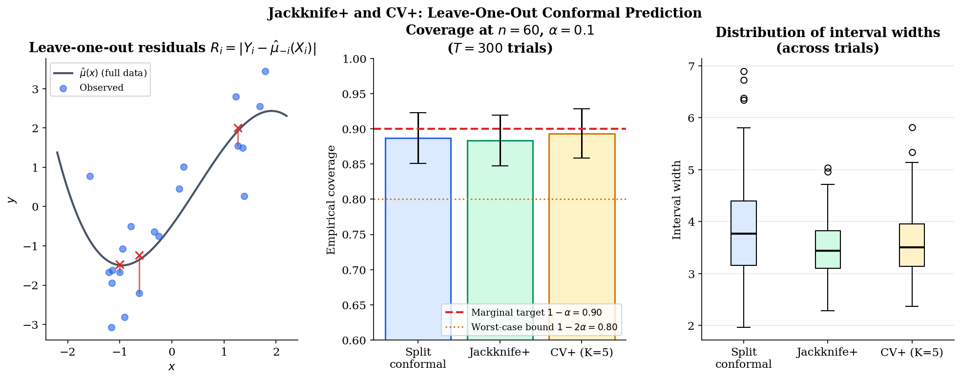
The empirical takeaway visible in the figure: at $n = 60$ — small enough that the calibration tax matters — jackknife+ and CV+ produce tighter intervals than split conformal at the same $\alpha$ , and the BCRT $1 - 2\alpha$ bound is loose by a wide margin. The choice between the three procedures is essentially a budget question. With abundant data and an expensive base predictor, split conformal is the workhorse. With a moderate $n$ and a cheap-to-refit predictor, jackknife+ extracts more from each observation. With expensive predictors but enough data to support fold-level fits, CV+ is the practical compromise.

What none of the three procedures achieve — and what §6 addresses — is locally adaptive width. Every procedure in §2–§5 produces a band whose half-width is a single global threshold; the band is wide where it doesn’t need to be (low-noise regions) and narrow where it shouldn’t be (high-noise regions). Conformalized quantile regression (CQR) fixes this by replacing the mean-residual nonconformity score with one built from quantile-regression endpoints.

Conformalized Quantile Regression (CQR)

The split-conformal interval $[\hat\mu(X_{n+1}) - \hat q_{1-\alpha},\ \hat\mu(X_{n+1}) + \hat q_{1-\alpha}]$ has the same half-width $\hat q_{1-\alpha}$ everywhere. On homoscedastic data this is fine — the conditional spread of $Y \mid X$ is constant by hypothesis. On heteroscedastic data it is wasteful where the noise is small and over-confident where the noise is large: the band over-covers in low-noise regions and under-covers in high-noise regions. The marginal coverage guarantee from Theorem 1 still holds — it is an average over the input distribution — but the conditional coverage at any specific $x$ can drift far from $1 - \alpha$ in either direction.

Conformalized quantile regression (Romano, Patterson & Candès 2019) keeps the conformal envelope but swaps the base learner. Instead of fitting a single mean predictor $\hat\mu$ , fit two quantile regressions — one estimating the lower conditional quantile $\hat q_{\alpha/2}(x)$ of $Y \mid X = x$ , the other estimating the upper conditional quantile $\hat q_{1-\alpha/2}(x)$ . The conditional QR endpoints already capture heteroscedasticity by design (they are wider where $Y \mid X$ is more dispersed); the conformal layer wraps them with a calibration step that preserves marginal coverage exactly. CQR thus inherits the distribution-free guarantee of split conformal and the locally adaptive width of quantile regression — the best of both worlds, with the only assumption still exchangeability.

Quantile regression itself is a topic for another day. For our purposes, treat $\hat q_{\alpha/2}(x)$ and $\hat q_{1-\alpha/2}(x)$ as black-box functions that take training data and return estimated conditional quantiles — fitted by check-loss minimization, possibly with regularization. Quantile Regression covers the estimation theory, asymptotic distribution, and broader applications.

Definition 4 (CQR Prediction Set).

Let $\hat q_{\alpha/2}(x)$ and $\hat q_{1-\alpha/2}(x)$ be quantile-regression estimates of the conditional $\alpha/2$ and $1 - \alpha/2$ quantiles of $Y \mid X = x$ , fit on the training set. For each calibration point $i$ , define the CQR nonconformity score

E_i \;=\; \max\bigl\{\, \hat q_{\alpha/2}(X_i) - Y_i,\ Y_i - \hat q_{1-\alpha/2}(X_i) \,\bigr\}.

The score $E_i$ is positive when $Y_i$ lies outside the QR interval $[\hat q_{\alpha/2}(X_i),\ \hat q_{1-\alpha/2}(X_i)]$ — measuring how far outside, in the direction of the violation — and negative when $Y_i$ lies inside. Let $\hat Q_{1-\alpha}$ denote the $\lceil (1-\alpha)(n_{\text{cal}} + 1) \rceil$ -th smallest of $(E_i)_{i=1}^{n_{\text{cal}}}$ . The CQR prediction set at test input $x$ is

\hat C_\alpha^{\text{CQR}}(x) \;=\; \bigl[\, \hat q_{\alpha/2}(x) - \hat Q_{1-\alpha},\ \hat q_{1-\alpha/2}(x) + \hat Q_{1-\alpha} \,\bigr].

The construction is mechanically simple: shift the lower QR endpoint down by $\hat Q_{1-\alpha}$ , shift the upper up by the same amount. If the QR fits are well-calibrated and most $Y_i$ already fall inside their intervals, then $E_i$ is negative for most $i$ , the empirical quantile $\hat Q_{1-\alpha}$ is small or even negative, and CQR produces an interval narrower than the QR interval itself (a tighter band, achievable because the calibration step “credits back” the QR’s natural slack). If the QR fits are systematically narrow or wrong, $E_i$ is positive for many $i$ , $\hat Q_{1-\alpha}$ is large and positive, and the CQR interval inflates the QR endpoints to recover the marginal-coverage guarantee. Either way, the band width is allowed to vary with $x$ — which is the locally adaptive property naive split conformal lacks.

α0.10noise h0.60

BothNaive onlyCQR only

Heteroscedasticity: σ(x) = 0.3 + h · |x|. At h = 0 the noise is constant and both bands are equivalent. As h grows, naive split-conformal's constant-width band over-covers near x = 0 and under-covers in the tails (visible in the right panel as a U-shaped dip below 1 − α). CQR's per-x quantile estimates track the noise envelope, keeping the right-panel curve much flatter — approximate conditional coverage as a side benefit of locally adaptive width.

Two-panel figure: left shows heteroscedastic regression data with naive split-conformal band (constant width, blue) and CQR band (locally adaptive, green) overlaid; right shows binned conditional coverage as a function of x for both methods with the nominal target line

CQR vs naive split conformal on heteroscedastic data, α = 0.10. Left: both bands achieve nominal marginal coverage, but the CQR band tracks the local noise envelope while the naive band carries a constant width. Right: binned conditional coverage as a function of x. Naive split conformal under-covers in the high-noise tails and over-covers near the low-noise center; CQR's curve is visibly flatter, achieving approximate conditional coverage as a side benefit of the locally adaptive width.

Theorem 3 (CQR Coverage Inheritance — Romano, Patterson & Candès 2019).

Under exchangeability of $(X_i, Y_i)_{i=1}^{n_{\text{cal}}+1}$ ,

\mathbb{P}\bigl( Y_{n_{\text{cal}}+1} \in \hat C_\alpha^{\text{CQR}}(X_{n_{\text{cal}}+1}) \bigr) \;\geq\; 1 - \alpha.

Proof.

CQR is split conformal applied to the nonconformity score

s(x, y) \;=\; \max\bigl\{\, \hat q_{\alpha/2}(x) - y,\ y - \hat q_{1-\alpha/2}(x) \,\bigr\}.

This score depends on the training set (through the fitted quantile regressions $\hat q_{\alpha/2}$ and $\hat q_{1-\alpha/2}$ ) but not on the calibration or test data — exactly the hypothesis of Theorem 1. The marginal-coverage statement therefore applies verbatim, giving $\mathbb{P}(Y_{n_{\text{cal}}+1} \in \hat C_\alpha^{\text{CQR}}) \ge 1 - \alpha$ . The two-sided refinement from Theorem 1 also extends: if the score distribution is continuous, coverage is bounded above by $1 - \alpha + 1/(n_{\text{cal}}+1)$ .

∎

Remark (CQR's Novelty Is the Score, Not the Theorem).

The proof of Theorem 3 is one paragraph because CQR is a special case of Theorem 1. The novelty of CQR is not a new probabilistic argument — it is the choice of score function. Naive split conformal with $s(x, y) = |y - \hat\mu(x)|$ produces an interval of constant half-width $\hat q_{1-\alpha}$ centered on $\hat\mu(x)$ . CQR replaces this with an interval whose endpoints are themselves regressed on $x$ : the lower endpoint is $\hat q_{\alpha/2}(x)$ shifted down by $\hat Q_{1-\alpha}$ , the upper is $\hat q_{1-\alpha/2}(x)$ shifted up. Because the QR estimates capture heteroscedasticity at the base-learner level, the conformal envelope inherits a locally adaptive width without any additional machinery. The lesson generalizes: any time you want a different shape of prediction interval, design the nonconformity score to extract that shape, and let Theorem 1 deliver the coverage guarantee for free.

Remark (Approximate Conditional Coverage).

CQR does not achieve exact conditional coverage — that is impossible for any distribution-free procedure with finite, informative prediction sets, as we will show in §8. It does achieve an empirically much flatter conditional-coverage curve than naive split conformal, in the sense that the gap $|\mathbb{P}(Y \in \hat C(X) \mid X = x) - (1 - \alpha)|$ is small on average over $x$ when the QR base learner is well-specified. The visualization above makes this precise on a heteroscedastic example: naive split conformal under-covers in the high-noise tails by 5–10 percentage points, while CQR holds within 2–3 percentage points across the input range. The improvement is empirical, not theoretical, and it depends on the QR fits being good enough to capture the conditional spread — which is itself a hard estimation problem for high-dimensional or low-data settings.

CQR is the practical default whenever the data is visibly heteroscedastic and computational budget allows fitting two quantile regressions. It is also the construction that points furthest in the direction of conditional coverage — a property that motivates the impossibility theorem of §8 and the importance-weighted extensions for known covariate shift. Before that, §7 takes the conformal envelope into a different setting entirely: classification, where the response is discrete and “interval” gets replaced by prediction set.

Adaptive Prediction Sets (APS) for Classification

Everything so far has been regression. Conformal prediction adapts to classification with a single change: replace the absolute-residual nonconformity score with one built on top of the classifier’s softmax probabilities. The output is no longer an interval — it is a set of predicted classes, sized to match the model’s uncertainty at the test input. Adaptive Prediction Sets (APS), due to Romano, Sesia & Candès (2020), is the canonical construction. Like CQR, it is split conformal applied to a different score, so Theorem 1 delivers the marginal coverage guarantee for free.

Setup. Let $\mathcal{Y} = \{1, \ldots, K\}$ be the discrete response space. A classifier produces softmax probabilities $\hat\pi(c \mid x) \in [0, 1]$ with $\sum_c \hat\pi(c \mid x) = 1$ . Order the classes at input $x$ from highest to lowest probability:

c_{(1)}(x),\ c_{(2)}(x),\ \ldots,\ c_{(K)}(x), \quad \hat\pi(c_{(1)} \mid x) \geq \hat\pi(c_{(2)} \mid x) \geq \cdots \geq \hat\pi(c_{(K)} \mid x).

For any class $y$ , write $\rho(y; x)$ for its rank in this descending ordering — so the most-probable class has rank 1, the second-most has rank 2, and so on.

Definition 5 (APS Score and Prediction Set, Deterministic Variant).

The APS nonconformity score at a labeled point $(x, y)$ is the cumulative mass of all classes ranked strictly above $y$ :

s(x, y) \;=\; \sum_{j=1}^{\rho(y; x) - 1} \hat\pi\bigl( c_{(j)}(x) \mid x \bigr).

The top-predicted class has score $0$ (no classes above it); the second has score $\hat\pi(c_{(1)} \mid x)$ ; and so on through the ordering. Given calibration scores $S_i = s(X_i, Y_i)$ for $i = 1, \ldots, n_{\text{cal}}$ , let $\hat q_{1-\alpha}$ denote the $\lceil (1 - \alpha)(n_{\text{cal}} + 1) \rceil$ -th smallest. The deterministic APS prediction set at a new test input $x$ is

\hat C_\alpha^{\text{APS}}(x) \;=\; \bigl\{\, c \in \mathcal{Y} \,:\, s(x, c) \le \hat q_{1-\alpha} \,\bigr\}.

Equivalently: include classes from highest probability downward until the cumulative mass of the strictly-higher classes exceeds the threshold.

α0.10class overlap σ1.00

Three Gaussian blobs at fixed centers; σ controls within-class spread (smaller = more separable, larger = more overlap). At small σ the classifier is confident almost everywhere and APS produces singletons; at large σ the decision boundaries get thick and the set sizes grow to 2 or 3 there. Marginal coverage tracks 1 − α regardless of σ; per-set-size coverage stays close to nominal — APS is not over-extracting coverage from any one set-size bucket.

Three-panel APS visualization on a 2D 3-class classification problem: classifier softmax shown as alpha-modulated colored regions on the left, APS region map colored by set size (1/2/3) in the middle, and a bar chart of empirical set-size distribution alongside per-set-size coverage on the right

APS on a 3-class 2D Gaussian-blob classification, α = 0.10. Left: classifier softmax — argmax color, alpha modulated by max probability. Middle: APS region map colored by set size (green = 1, amber = 2, red = 3). Set sizes grow at the decision boundaries where the classifier is genuinely uncertain. Right: empirical set-size distribution on a held-out test set, plus per-set-size coverage. Marginal coverage matches the 0.90 target; conditional coverage given set size is also close to nominal — APS adapts where adaptation is needed.

The deterministic APS variant always includes the top-predicted class (its score is $0 \le \hat q_{1-\alpha}$ for any non-trivial threshold), so $\hat C_\alpha^{\text{APS}}$ is never empty. Romano-Sesia-Candès also describe a randomized variant that achieves exactly $1 - \alpha$ coverage by allowing the borderline class to be included with a probability tuned to the calibration set; the deterministic version overcovers by at most $\frac{1}{n_{\text{cal}} + 1}$ — the same discretization slack we saw in Theorem 1’s upper bound — and is the version implemented in libraries like mapie.

Coverage. APS is split conformal with the score above. The score depends only on the training-fitted classifier (and therefore not on the calibration or test data), so Theorem 1 applies verbatim and gives

\mathbb{P}\bigl( Y_{n_{\text{cal}}+1} \in \hat C_\alpha^{\text{APS}}(X_{n_{\text{cal}}+1}) \bigr) \;\geq\; 1 - \alpha,

with the same two-sided refinement $\le 1 - \alpha + 1/(n_{\text{cal}}+1)$ when scores are continuous. (For APS the score is discrete by construction — it takes at most $K$ distinct values per input — so the upper bound holds with the discrete analog: ties between calibration scores can be broken with the deterministic-rule convention with no impact on the lower bound.)

Why APS, not top-K? A naive alternative is “include the smallest set of classes whose cumulative softmax mass exceeds $1 - \alpha$ .” This is the top- $K$ procedure where $K$ varies per input. It works when the classifier’s softmax is well-calibrated — meaning the predicted probabilities match the true conditional probabilities $\mathbb{P}(Y = c \mid X = x)$ — but degrades sharply when softmax is miscalibrated, which is the typical case for modern neural networks. APS is the calibrated alternative: the threshold $\hat q_{1-\alpha}$ is determined empirically from the calibration set rather than implicitly through the softmax magnitudes, so coverage is decoupled from softmax-calibration assumptions. Whatever the classifier’s calibration quality, APS recovers the marginal-coverage guarantee.

Adaptivity. The set size at any test input is exactly the number of classes $c$ with $s(x, c) \le \hat q_{1-\alpha}$ — equivalently, the smallest $K^\ast$ such that $\sum_{j=1}^{K^\ast - 1} \hat\pi(c_{(j)} \mid x) > \hat q_{1-\alpha}$ . Where the classifier is confident ( $\hat\pi(c_{(1)}) \approx 1$ ), the second class already has score $\approx 1 > \hat q_{1-\alpha}$ (typically), so the set is a singleton. Where the classifier is genuinely uncertain across multiple classes, the top score grows slowly and several classes pass the threshold, producing a multi-class set. Romano-Sesia-Candès 2020 prove that APS achieves approximate conditional coverage when softmax is well-calibrated — the average gap $|\mathbb{P}(Y \in \hat C(X) \mid X = x) - (1 - \alpha)|$ is small — though, as with CQR, exact conditional coverage is impossible by the result we turn to next.

The figure above is worth pausing on. The middle panel — the region map colored by set size — is the most direct visualization of what APS is doing. Inside each class blob the set is a singleton (green); along the decision boundaries between blobs, where two classes are competitive, the set grows to two (amber); in the central region where all three classes are roughly equally probable, the set grows to three (red, when present). The bar chart on the right confirms the marginal coverage and shows that per-set-size coverage is also close to $1 - \alpha$ — the procedure is not gaming the average by extracting all its coverage from one set-size bucket.

APS extends to multi-label classification, ordinal classification, and hierarchical class structures — each by appropriate redesign of the nonconformity score. The pattern from §6 holds: the score does the work, and Theorem 1 delivers the guarantee. Where the difficulty really lies is the conditional coverage problem: APS approximates it, but it cannot be achieved exactly without distributional assumptions. The next section makes that precise.

Conditional Coverage: Impossibility and Approximations

Theorem 1 guarantees marginal coverage: averaged over the joint distribution of training, calibration, and test data, the prediction set covers $Y_{n+1}$ with probability at least $1 - \alpha$ . The marginal probability is computed over the distribution of $X$ , so a procedure that systematically under-covers in one input region and over-covers in another can still satisfy Theorem 1. A user typically wants more — conditional coverage,

\mathbb{P}\bigl( Y_{n+1} \in \hat C_\alpha(X_{n+1}) \,\big|\, X_{n+1} = x \bigr) \;\geq\; 1 - \alpha \quad \text{for } P_X\text{-almost every } x. \tag{$\ast\ast$}

Conditional coverage means the procedure works uniformly across the input space: no input region is systematically undercovered. CQR and APS are designed with this property in view, and they achieve it approximately under reasonable assumptions on the base learner. The result of this section is that exact conditional coverage — the bound at $(\ast\ast)$ for every $x$ , distribution-free — is impossible for any procedure that produces finite, informative prediction sets. Foygel-Barber et al. 2021 made this precise by exhibiting an adversarial family of distributions on which any conditionally-valid procedure must produce arbitrarily wide intervals at the adversarial input.

Theorem 4 (Conditional Coverage Impossibility — Foygel Barber, Candès, Ramdas & Tibshirani 2021).

Let $\mathcal{P}$ be a class of distributions on $\mathbb{R} \times \mathbb{R}$ satisfying:

(i) $X$ has a continuous distribution under each $P \in \mathcal{P}$ ;

(ii) $\mathcal{P}$ is closed under spiked-variance perturbations: for any $\sigma_0, M > 0$ , $x_0 \in \mathbb{R}$ , and $\varepsilon > 0$ , the distribution

X \sim \text{Uniform}[-1, 1], \quad Y \mid X = x \sim N\!\bigl(0,\ \sigma_0^2 + M^2 \cdot \mathbb{1}\{|x - x_0| < \varepsilon/2\} \bigr)

belongs to $\mathcal{P}$ .

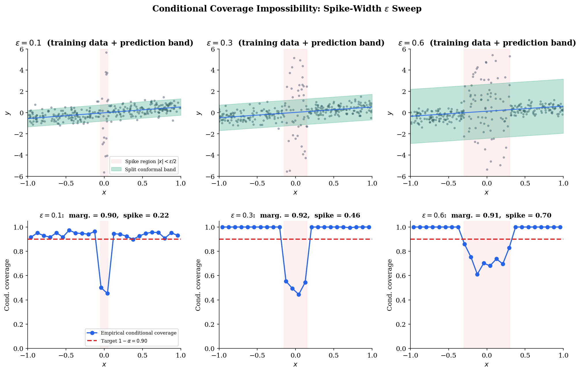
Suppose $\hat C_\alpha$ is a (data-dependent) prediction procedure satisfying conditional coverage $(\ast\ast)$ uniformly over $\mathcal{P}$ . Then for any fixed sample size $n$ and any $\delta > 0$ , there exists a distribution $P_0 \in \mathcal{P}$ (with spike width $\varepsilon \le \delta$ ) such that, with probability at least $1/2$ over the calibration data,

\text{Lebesgue}\bigl( \hat C_\alpha(x_0) \bigr) \;\geq\; 2 \Phi^{-1}(1 - \alpha/2) \sqrt{\sigma_0^2 + M^2},

where $\Phi$ is the standard normal CDF. As $M$ can be taken arbitrarily large, the expected Lebesgue measure of $\hat C_\alpha(x_0)$ under $P_0$ is unbounded.

Proof.

The argument is constructive. Fix the sample size $n$ and the resolution parameter $\delta > 0$ . We will exhibit a member of $\mathcal{P}$ on which any conditionally-valid procedure must produce an arbitrarily wide prediction set at $x_0 = 0$ .

Step 1: Choose the spike. Set $\varepsilon = \min(\delta, 1/n)$ . Let $P_0$ be the spiked-variance distribution from condition (ii) with spike center $x_0 = 0$ , spike width $\varepsilon$ , baseline noise $\sigma_0$ , and spike magnitude $M$ (to be sent to infinity at the end). Under $P_0$ , the conditional distribution at $x = 0$ — the spike center — is $N(0, \sigma_0^2 + M^2)$ , while at any $x$ outside the spike interval $[-\varepsilon/2, \varepsilon/2]$ the conditional distribution is $N(0, \sigma_0^2)$ .

Step 2: The “no spike samples” event $A$ . Each draw $(X_i, Y_i)$ has $X_i$ in the spike interval with probability $\varepsilon/2$ (the interval has length $\varepsilon$ and $X$ is uniform on $[-1, 1]$ ). The probability that no calibration point falls in the spike interval is

\mathbb{P}(A) \;=\; (1 - \varepsilon/2)^{n_{\text{cal}}} \;\geq\; (1 - 1/(2n))^{n} \;\to\; e^{-1/2} \;\approx\; 0.61

as $n \to \infty$ . For moderate $n$ — and for our $\varepsilon \le 1/n$ — this probability exceeds $1/2$ . So with probability at least $1/2$ over the calibration data, no observation in the calibration set is informative about the spike.

Step 3: Indistinguishability. Let $Q$ denote the spike-free baseline distribution: $X \sim \text{Uniform}[-1, 1]$ , $Y \mid X \sim N(0, \sigma_0^2)$ , no spike. On the event $A$ (no calibration point lands in the spike), the calibration data is observationally indistinguishable from a sample drawn under $Q$ — every observed pair $(X_i, Y_i)$ is consistent with both $P_0$ and $Q$ . Because $\hat C_\alpha$ is a measurable function of the calibration data, on the event $A$ the procedure produces the same prediction set it would have produced under $Q$ :

\hat C_\alpha \big|_{A} \;=\; \hat C_\alpha^{(Q)}

with $\hat C_\alpha^{(Q)}$ denoting the procedure’s output when calibrated under $Q$ . The procedure cannot tell which distribution it is operating under because the calibration data does not separate them.

Step 4: Conditional coverage at the spike. Now condition on event $A$ and on the test input $X_{n+1} = x_0 = 0$ . Under the true distribution $P_0$ , the conditional law $Y_{n+1} \mid X_{n+1} = x_0$ is $N(0, \sigma_0^2 + M^2)$ — full spike variance. The conditional-coverage hypothesis $(\ast\ast)$ requires

\mathbb{P}\bigl( Y_{n+1} \in \hat C_\alpha^{(Q)}(x_0) \,\big|\, A,\ X_{n+1} = x_0 \bigr) \;\geq\; 1 - \alpha,

where we have substituted $\hat C_\alpha = \hat C_\alpha^{(Q)}$ from Step 3. The left side is the probability that an $N(0, \sigma_0^2 + M^2)$ random variable lies in a fixed (data-dependent) set $\hat C_\alpha^{(Q)}(x_0)$ .

Step 5: Anderson’s lemma. For any measurable $S \subseteq \mathbb{R}$ with $\mathbb{P}(Z \in S) \ge 1 - \alpha$ where $Z \sim N(0, \tau^2)$ , the Lebesgue measure of $S$ is bounded below by the Lebesgue measure of the smallest symmetric interval centered at the mode containing the same probability mass:

\text{Lebesgue}(S) \;\geq\; 2 \Phi^{-1}(1 - \alpha/2) \cdot \tau.

(This is Anderson’s lemma applied to a unimodal Gaussian: among all sets of prescribed measure, the central interval maximizes the Gaussian probability; equivalently, among all sets of prescribed Gaussian probability, the central interval minimizes Lebesgue measure.) Applied to $S = \hat C_\alpha^{(Q)}(x_0)$ and $\tau^2 = \sigma_0^2 + M^2$ :

\text{Lebesgue}\bigl( \hat C_\alpha^{(Q)}(x_0) \bigr) \;\geq\; 2 \Phi^{-1}(1 - \alpha/2) \sqrt{\sigma_0^2 + M^2}.

Step 6: Send $M \to \infty$ . The right side grows without bound as $M$ increases, and the inequality holds on the event $A$ (probability at least $1/2$ ). The expected Lebesgue measure of $\hat C_\alpha(x_0)$ under $P_0$ is therefore unbounded, completing the construction.

∎

Remark (Impossibility Holds with Only Measurability).

The proof never invokes any regularity property of the procedure $\hat C_\alpha$ beyond its being a measurable function of the calibration data. The argument does not assume the procedure is symmetric, exchangeable, or based on any specific score; it does not assume the predictor $\hat\mu$ is consistent or unbiased; it does not even assume $\hat C_\alpha$ produces an interval (it works for arbitrary measurable subsets of $\mathbb{R}$ ). The “no spike samples” event $A$ does the entire heavy lifting: on $A$ , the calibration data does not separate $P_0$ from $Q$ , so any procedure computed only from data cannot discriminate between the two — yet $(\ast\ast)$ at $x_0$ requires distinguishing them. The impossibility is a statement about the information content of the calibration data, not about the procedure’s design.

Remark (Approximate Conditional Coverage of CQR/APS).

Theorem 4 does not contradict §6 (CQR) or §7 (APS). Both procedures retain marginal coverage — Theorem 1 still applies — and produce adaptive prediction sets whose width or size varies with $x$ . What they do not claim is conditional coverage uniformly over the spiked-variance family $\mathcal{P}$ . Under additional smoothness assumptions on $Y \mid X$ — assumptions that exclude spiked-variance distributions, such as Lipschitz continuity of the conditional CDF — CQR achieves an approximate conditional-coverage guarantee in which the average gap

\mathbb{E}_{X}\Bigl[\, \bigl| \mathbb{P}(Y \in \hat C(X) \mid X) - (1 - \alpha) \bigr| \,\Bigr]

is small. The empirical message of §6’s CQR-vs-naive comparison was exactly this: under reasonable conditions, CQR’s per-bin coverage curve is much flatter than naive split conformal’s. Theorem 4 says: drop the smoothness assumptions and adversarial constructions reassert themselves. Any practical claim to “conditional coverage” implicitly invokes such assumptions.

Six-panel figure organized as 2 rows by 3 spike-width values: top row shows training data with the spike region shaded and the split conformal prediction band overlaid; bottom row shows binned conditional coverage as a function of x, demonstrating that marginal coverage holds at every spike width but conditional coverage on the spike region degrades as the spike narrows — The impossibility theorem made tangible. Three spike widths ε ∈ {0.10, 0.30, 0.60}, with split conformal applied at α = 0.10. Top row: training data and prediction bands — the band has constant width regardless of spike width, because the calibration set rarely sees the spike. Bottom row: empirical conditional coverage as a function of x. Marginal coverage holds at the 0.90 target in every panel; conditional coverage on the spike region collapses as ε shrinks (the procedure has no information to widen the band where it should). At ε = 0.10 the spike-region coverage is far below nominal.

Remark (Covariate Shift Connection — Tibshirani, Foygel Barber, Candès & Ramdas 2019).

The impossibility motivates an extension that has become the standard fix when the user has known distribution-shift information. If the test distribution $P_X^{\text{test}}$ differs from the training distribution $P_X^{\text{train}}$ , exchangeability fails and naive split conformal can lose its marginal coverage at the test distribution. Tibshirani, Foygel Barber, Candès & Ramdas (NeurIPS 2019) showed that importance-weighted split conformal — where calibration scores are weighted by the likelihood ratio $w(x) = p_{\text{test}}(x) / p_{\text{train}}(x)$ — restores marginal coverage at the test distribution under known shift. The construction is the weighted empirical quantile of the calibration scores, with the test point’s own weight entering the denominator (this is the weightedSplitConformal in nonparametric-ml.ts). It does not solve the conditional-coverage problem of Theorem 4 — that remains impossible — but it does solve the marginal-coverage-under-shift problem, which is the more practical concern in many deployment settings.

shift Δ0.50α0.10

BothNaive onlyWeighted only

Train distribution: x ~ N(0, 1), blue histogram. Test distribution: x ~ N(Δ, 1), green histogram. Naive split conformal (blue band) was calibrated on the train distribution and progressively under-covers as Δ grows — the bottom-panel blue curve drops well below 1 − α. The TBCR 2019 importance-weighted variant (green band) uses the closed-form Gaussian density ratio w(x) = N(x; Δ, 1) / N(x; 0, 1) to recalibrate; the bottom-panel green curve holds at the 1 − α target across the entire shift range.

The takeaway from §8 is paired. Negative: distribution-free conditional coverage is impossible at full generality; any procedure claiming it must restrict to a smaller distribution class. Positive: marginal coverage under shift is recoverable when the shift is known, via importance-weighted variants of the procedures we’ve already developed. Conditional coverage in practice is achieved approximately by adaptive base learners (CQR, APS) and assessed empirically — an honest report of the per-region coverage gap, not a theoretical guarantee. With these limits drawn, §9 returns to the practical question that motivated the topic: how do we wrap conformal prediction around any black-box ML model?

Wrapping Black-Box ML Models

The whole point of conformal prediction’s distribution-free guarantee is that the base predictor can be anything — ridge regression, gradient boosting, random forest, neural network, transformer, anything that maps inputs to predictions. Theorem 1 doesn’t care what’s inside; it only cares that the score function is held fixed across calibration and test. This means the entire topic up to here applies, unchanged, to any model you already have.

The skeleton in five steps:

Step 1 — Split. Partition your data into training, calibration, and test (typically 50/50 between the first two; test is whatever you want to evaluate on later).

Step 2 — Fit. Train your favorite black-box model $\hat\mu$ on the training set. Hyperparameter tuning, early stopping, ensembling — all fine, as long as none of it touches the calibration set.

Step 3 — Score. Compute calibration scores $S_i = |Y_i - \hat\mu(X_i)|$ on the calibration set (or the CQR/APS variants from §6/§7 if you want adaptivity).

Step 4 — Threshold. Set $\hat q_{1-\alpha}$ to the $\lceil (1-\alpha)(n_{\text{cal}} + 1) \rceil$ -th smallest calibration score.

Step 5 — Predict. For each new test point $X_{n+1}$ , return $\hat C_\alpha(X_{n+1}) = [\hat\mu(X_{n+1}) - \hat q_{1-\alpha},\ \hat\mu(X_{n+1}) + \hat q_{1-\alpha}]$ (or the appropriate analog for your score function).

That is the entire procedure. There are no model-class-specific tweaks; ridge and a 100-million-parameter transformer use the same five steps. The cost of conformal wrapping is one calibration pass and one threshold lookup — additive overhead measured in milliseconds for any non-trivial base predictor.

The empirical demonstration in Figure 9 below applies these five steps to three base predictors on the same heteroscedastic regression dataset: a degree-3 polynomial ridge (the predictor we have used throughout), a small MLP with two hidden layers, and a random forest. All three target $\alpha = 0.10$ and all three achieve empirical marginal coverage near 0.90 — the conformal layer enforces the guarantee regardless of the base predictor’s particulars. What does vary across predictors is the width of the prediction interval: the better-fit predictor produces tighter intervals because its residuals on the calibration set are smaller, so $\hat q_{1-\alpha}$ shrinks. Width depends on accuracy, coverage does not — a one-line summary of what conformal prediction buys you.

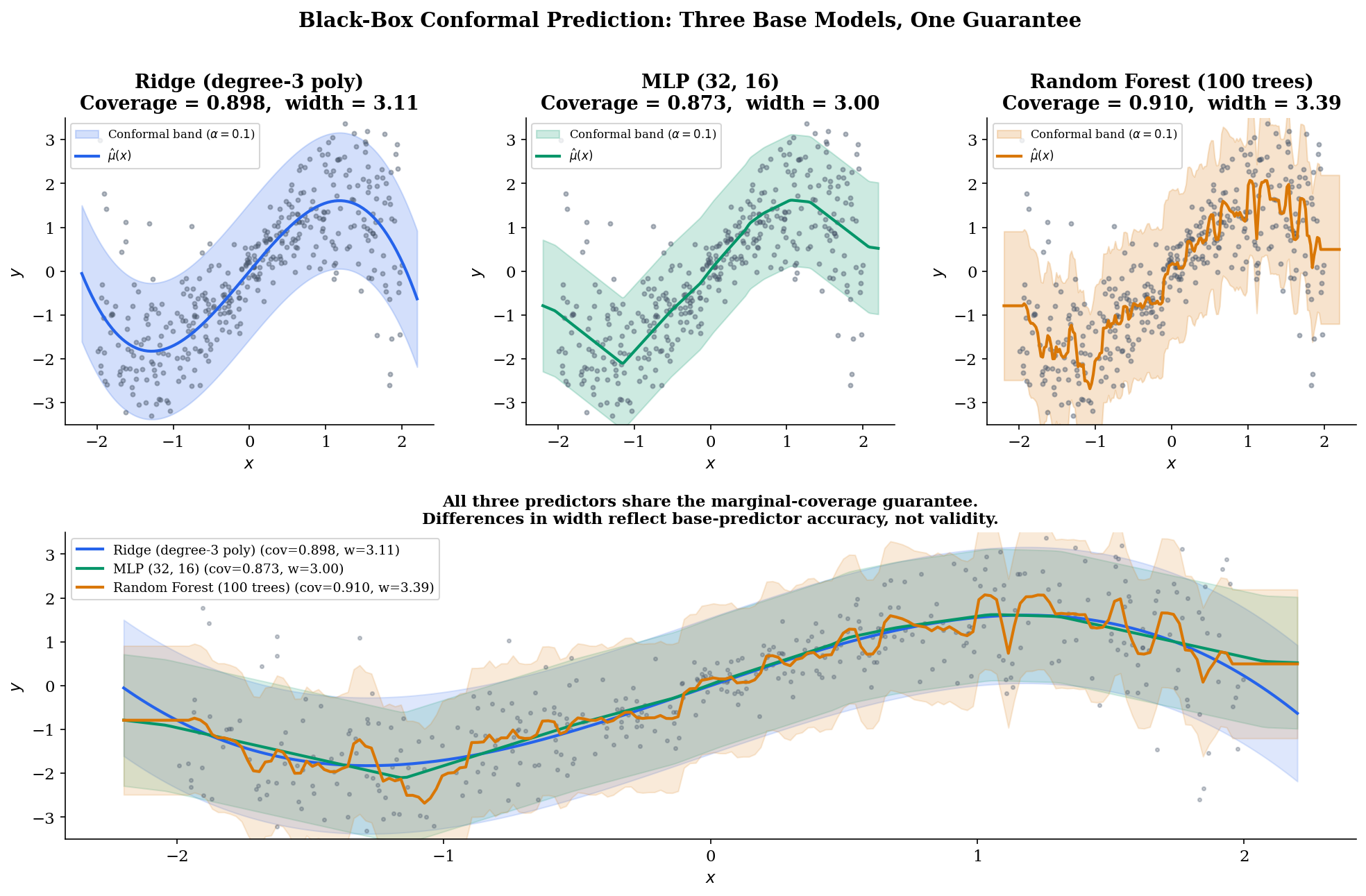
Four-panel figure: top row shows three predictor-specific prediction bands (ridge, MLP, random forest) on the same heteroscedastic data with each panel reporting empirical coverage and mean width; bottom panel overlays all three bands for direct visual comparison — Three base predictors, one conformal envelope, α = 0.10. Top row: ridge (blue), MLP (green), random forest (amber) — each panel reports empirical coverage and mean band width. All three land at ~0.90 coverage on the held-out test set. Bottom: direct overlay. The widths differ because the residuals do; the coverage doesn't differ because the conformal calibration step doesn't care which predictor produced the residuals.

For production deployments, the mapie library implements split conformal, jackknife+, CQR, and APS (deterministic and randomized) for arbitrary scikit-learn estimators with a few-line API. The Python reference implementation in this topic’s notebook uses mapie for the §9 black-box demonstration — the same pattern carries to PyTorch and JAX models with minimal adaptation. Conformal prediction is one of the rare statistical guarantees that scales from $n = 50$ toy datasets to $n = 10^9$ industrial pipelines without changing its assumptions or its math.

The wrapping pattern also extends in directions we have only sketched. Online conformal prediction (Vovk-Gammerman-Shafer 2005, Gibbs-Candès 2021) updates the threshold as new data arrives, retaining marginal coverage even when the data stream has slow distribution drift. Conformal prediction for time series handles non-exchangeable streams via blocked or weighted variants. Conformal classification with structured output spaces (multi-label, hierarchical, set-valued) generalizes APS by redesigning the score for each setting. None of these change the five-step skeleton above; they swap the score, the calibration step, or the data assumption — and let the marginal-coverage theorem do its work.

Notation Reference

The symbols used throughout this topic, gathered for quick lookup. The “Connections” and “References & Further Reading” sections that follow are auto-generated from the topic frontmatter; the related-topics relationships expressed there are the structured form of the cross-references made inline in §1, §6, and §8.

Symbol	Meaning
$(X_i, Y_i)$	Feature–response pair, $X_i \in \mathcal{X}$ , $Y_i \in \mathcal{Y}$ .
$n_{\text{cal}}$	Calibration set size.
$\alpha \in (0, 1)$	Miscoverage level; nominal coverage is $1 - \alpha$ .
$\hat\mu(x)$	Fitted base predictor (training data only, in the split case).
$s(x, y)$	Nonconformity score; large = anomalous.
$S_i = s(X_i, Y_i)$	Calibration score at observation $i$ .
$\hat q_{1-\alpha}$	Threshold: the $\lceil (1-\alpha)(n_{\text{cal}}+1) \rceil$ -th smallest of $\{S_i\}$ .
$\hat C_\alpha(x)$	Prediction set: $\{y \in \mathcal{Y} : s(x, y) \le \hat q_{1-\alpha}\}$ .
$R_i$	Leave-one-out residual (jackknife+ / CV+).
$\hat Q_\alpha^-,\ \hat Q_{1-\alpha}^+$	Empirical quantiles with floor/ceiling conventions (jackknife+).
$\hat q_{\alpha/2}(x),\ \hat q_{1-\alpha/2}(x)$	Conditional quantile estimates (CQR base learner).
$E_i$	CQR nonconformity score at observation $i$ .
$\hat\pi(c \mid x)$	Predicted softmax probability of class $c$ at input $x$ (APS).
$c_{(j)}(x)$	$j$ -th most probable class at $x$ .
$\rho(y; x)$	Rank of class $y$ in the descending probability ordering.
$\sigma^2(x; \varepsilon)$	Spiked-variance adversarial family from the Theorem 4 proof.
$\Phi^{-1}$	Standard normal inverse CDF (Anderson’s lemma in Theorem 4).

Forward Connections to Planned formalML Topics

Three topics in the T4 Nonparametric & Distribution-Free track that pick up where this one leaves off. Plain-text references — links will activate as the topics ship.

Quantile Regression — the base learner inside CQR (§6). The full topic covers QR estimation theory, the asymptotic distribution of $\hat\beta(\tau)$ , regularized variants (lasso, group lasso) for high dimensions, and the broader use of quantile regression beyond the conformal envelope.

Statistical Depth (coming soon) — depth-based prediction regions are the geometric alternative to the score-based conformal construction. For symmetric distributions the two routes reproduce each other; for asymmetric ones they diverge instructively, with depth regions tracking the geometric center of mass and conformal sets tracking the score quantile. The cross-fertilization runs both ways.

Prediction Intervals (coming soon) — the umbrella topic that positions conformal prediction inside the broader prediction-interval ecosystem (frequentist plug-in, Bayesian posterior predictive, quantile-regression direct, conformal). Each route has different assumptions and different asymptotic properties; the comparative table is the topic’s central contribution.