Extreme Value Theory
Asymptotic theory of sample maxima and tail-based inference — Fisher–Tippett–Gnedenko trichotomy, generalized Pareto distribution, peaks-over-threshold, tail-index estimation, and ML applications including tail-aware prediction intervals, OOD detection, and tail-risk quantification
1. From the center to the tails
This section motivates the topic by drawing a clean parallel to the central limit theorem, sets up the formal target object (a non-degenerate limit law for the normalized sample maximum), introduces the running example that threads §§2–5, and previews where extreme value theory shows up in modern ML practice.
1.1 The companion to the central limit theorem
The central limit theorem classifies the limit distribution of one specific summary of an iid sample — the mean — by reducing an infinite-dimensional limit problem to a two-parameter family. The statement: as long as the second moment is finite, converges in distribution to regardless of what the underlying iid law is. The result is universal in a strong sense — the shape of the limit (Gaussian) doesn’t depend on the parent distribution at all; only the parameters and do.
Extreme value theory is the analogous story for a different summary: the maximum. Given iid , the sample maximum is a perfectly well-defined random variable, and the question of how behaves as has an answer of exactly the same shape as CLT’s. There is a finite-dimensional family of limit distributions — a three-parameter family this time, the generalized extreme value (GEV) distribution — and any non-degenerate limit of normalized sample maxima must lie in that family. This is the Fisher–Tippett–Gnedenko trichotomy of §2, the load-bearing result of the topic.
The parallel is worth holding in mind throughout. CLT and EVT are two faces of the same kind of theorem: take an iid sample, take a specific functional of the sample (mean for CLT, max for EVT), normalize affinely, and ask what the limit distribution looks like. In both cases, the answer is universal; the universality is the surprising part. CLT’s universality depends on the parent distribution’s second moment; EVT’s, on the rate at which its upper tail decays. We will see in §3 that the tail-decay condition partitions all “reasonable” parent distributions into three buckets, and the bucket determines which member of the GEV family shows up as the limit.
A warning before we set up the formalism. CLT-flavored intuition suggests that the bulk of the distribution should determine ‘s asymptotic behavior. It does not. The mean averages over the bulk; doubling halves the mean’s variance regardless of the parent distribution. The maximum picks a single observation, and not a representative one — its behavior is governed entirely by the right tail. Two distributions can be nearly identical in their first ninety-nine percentiles and have wildly different maxima. The classical illustration is Normal versus : both are symmetric, both have moderate variance, and CLT applies to both. But the maximum of iid standard normals grows like — slowly — while the maximum of iid samples grows like , polynomially. The difference is invisible until one specifically looks at the tail. It is the same gap that drives the heavy-tailed regime of prediction-intervals §4: split-conformal coverage holds for residuals as it does for Gaussian residuals, but the resulting interval is much wider because the tail is much heavier. EVT will give us the language to quantify the extent of the widening.
1.2 The target object
Let be iid with common CDF , and define the running maximum . Independence lets us compute ‘s CDF exactly:
This is the unnormalized answer, and on its own it carries no useful asymptotic information. For any in the interior of ‘s support, and so . For any (the upper endpoint of , possibly ), . The unnormalized converges in probability to the constant , a degenerate limit that contains no distributional information at all.
Affine normalization rescues us. We seek sequences and such that
at every continuity point of some non-degenerate limit CDF . The point of the normalization is to track on a scale where its distribution stabilizes — directly analogous to normalizing by in CLT.
Two observations about this setup that will matter in §2.
First, the choice of is not unique. If is a valid limit under , then for any the affinely transformed CDF is also a valid limit under sequences . So the shape of — its equivalence class under the affine transformation — is what’s universal, not the specific representative. The convergence-of-types lemma in §2 will turn this informal observation into a usable tool.
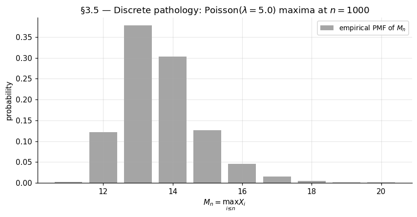
Second, not every admits a non-degenerate normalization. The pathological cases are essentially distributions whose tails decay too irregularly to admit a clean asymptotic shape. A concrete example: a Poisson distribution. We will see in §3 why; for now, the qualitative picture is that integer-valued distributions with light tails leave jumping discretely between consecutive integers in a way that no affine rescaling can smooth out. The set of for which a non-degenerate exists is exactly the domain of attraction of some GEV member, and the trichotomy of §2 says these domains exhaust everything reachable.
1.3 Running example: block maxima of iid standard normals
The single example that threads the entire topic is block maxima of iid standard normals. It is the simplest non-trivial parent distribution for which the limit theory bites, and every key construction (block-maxima fitting in §4, POT in §5, tail-index estimation in §5.4) reuses it as the calibration baseline.
For , the right normalization is
under which
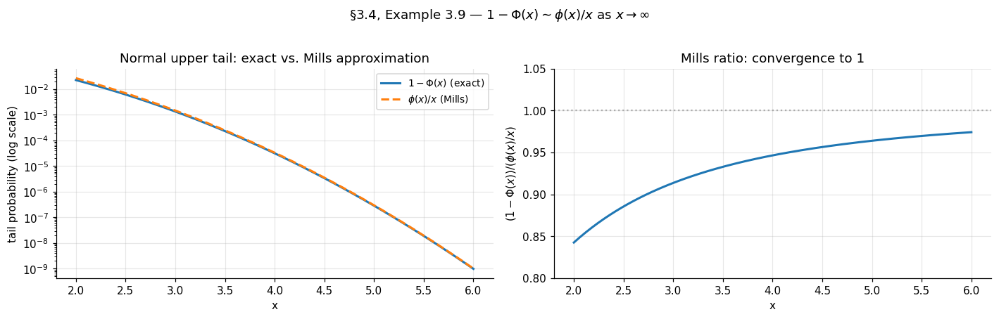
The limit is the standard Gumbel distribution. The derivation is a careful expansion of the Mills-ratio asymptotic for the Normal upper tail: as , where and are the standard Normal density and CDF. We reproduce the derivation in §3 once the regular-variation machinery is in place; for now, we take the result on faith and check it numerically.
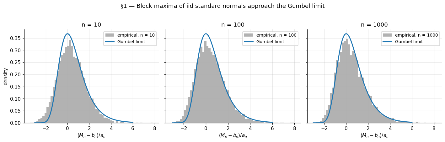
A few features of this normalization are worth pausing on. The location grows like , slowly. With , the typical maximum of iid standard normals is around ; doubling to moves it to about . The maximum drifts off to infinity, but extremely slowly. The scale shrinks at the same rate, so the spread of the maximum on its native scale also vanishes — but the affine rescaling exposes a stable shape, the Gumbel, with support on all of and double-exponentially decaying tails on both sides.
The convergence is visibly slow. The §1 figure shows histograms of at overlaid with the Gumbel density. At , the empirical distribution is noticeably to the left of the limit; at , the agreement is decent in the body and poor in the right tail; at , the match is good across most of the range. This slow convergence is generic — not a failure of the example — and we will return to it in §3 when we compute the convergence rate explicitly.
1.4 Where this matters: ML applications
Three application areas thread the topic and motivate why an ML practitioner should care.
Tail-aware prediction intervals. When residuals are heavy-tailed — the regime in prediction-intervals §4 is the canonical example — central-limit-flavored confidence bounds on the conditional mean systematically undershoot the actual coverage of prediction intervals. The Fréchet limit (§2) gives a principled way to quantify how far the tail extends and to construct prediction intervals that respect it. We return to this in §6.
Out-of-distribution detection. In production ML systems, OOD inputs often manifest as extreme values of some scalar score — softmax confidence, energy, reconstruction error, embedding norm. Modeling the tail of the in-distribution score with the GPD of §5 turns “score is unusually large” into a calibrated probability statement. This is the EVT reformulation of the classical softmax baseline.
Tail-risk quantification. Deployed models have failure modes that show up at the tail of some loss distribution — a 99.9th-percentile latency, a worst-case cost, a maximum classification error over a year. Estimating these from a finite sample requires extrapolating beyond the empirical tail, which is what fitted GEV/GPD models provide. The Value-at-Risk and Expected Shortfall computations in §5.6 are the canonical instances.
These three threads stay in the background through §§2–5 as we develop the asymptotic theory, and return to the foreground in §6.
2. Max-stability and the Fisher–Tippett–Gnedenko trichotomy
This is the load-bearing section of the topic. We define max-stability, prove that any non-degenerate limit law for normalized sample maxima must be max-stable, develop the type-convergence (Khintchine) lemma that powers the proof, and use these tools to state the Fisher–Tippett–Gnedenko theorem and its unified GEV parametrization. The classification proof is sketched in detail through the multiplicativity-of-scaling-coefficients argument that bridges the functional equation to the three families; the closing case work is referenced to Embrechts, Klüppelberg, and Mikosch §3.2 for full exhaustiveness.
2.1 Max-stability
The definition is the natural notion of “stability under taking maxima,” directly parallel to stability under sums.
Definition 1 (Max-stability).
A non-degenerate CDF on is max-stable if for every integer there exist constants and such that
The relation has a clean probabilistic reading. If are iid with CDF , the maximum has CDF . Setting and rearranging gives , i.e., has the same distribution as , a single affinely shifted. Taking the maximum of copies is, up to known affine recalibration, statistically equivalent to scaling and shifting one copy. The defining feature of CLT’s Gaussian — that taking sums and rescaling preserves shape — has its analog here, with maxima instead of sums, in rather than .
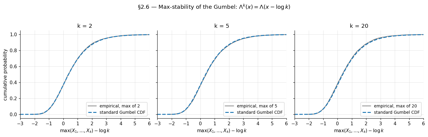
A worked example fixes ideas. The standard Gumbel from §1 satisfies
So is max-stable with — taking the max of iid Gumbels just shifts the location by with no rescaling. The other two families we will meet (Fréchet and reverse-Weibull) are also max-stable with their own patterns; the figure below verifies the Gumbel relation numerically.
The standard Normal , by contrast, is not max-stable. The maximum of iid standard normals does not have the same distribution as any affine recalibration of a single standard normal — its tail is too thin in a different way. The §1 example showed this concretely: the Normal-block-maxima limit is Gumbel, not Normal. So the parent distribution and the limit distribution genuinely differ; the limit picks up a structural property (max-stability) that the parent lacks.
2.2 Any non-degenerate limit must be max-stable
The first half of Fisher–Tippett–Gnedenko is the implication “limit ⟹ max-stable.” It is a short, clean argument once the type-conversion lemma is in place.
Theorem 1 (Necessity of max-stability).
Suppose are iid with CDF , and that for some sequences and some non-degenerate CDF ,
at every continuity point of . Then is max-stable.
Proof.
The strategy is to look at sample sizes that are products: replace by for a fixed positive integer , and compute the limit of under two different normalizing schemes. The two schemes converge to two different (but type-equivalent) limits; the type-convergence lemma will tell us how to relate them, and that relationship will be the max-stability functional equation.
Scheme 1 — block-of-blocks. Partition the first observations into disjoint blocks of size , write for the per-block maxima, and observe that . By independence the are iid with CDF , so
By hypothesis, the inner expression converges to , so by continuous-mapping
at every continuity point of — equivalently, of , since has the same continuity set as .
Scheme 2 — direct. Apply the original hypothesis with replaced by (a valid substitution since as for fixed ). This gives
i.e., .
Combining. We have the same sequence converging to two non-degenerate limits under two affine renormalizations: to under and to under . The type-convergence lemma (Lemma 1 below) takes this input precisely. It guarantees that and for some , and that the two limits are related by
This is the defining functional equation of Definition 1. Since was arbitrary, is max-stable.
∎The proof did not use any property of beyond the convergence hypothesis. Whatever the parent is, if the normalized maximum has a non-degenerate limit, that limit is max-stable. The constraints on the limit are entirely structural.
2.3 The type-convergence lemma
The lemma the necessity proof leans on is Khintchine’s convergence of types. It is a general statement about how affine renormalizations of one sequence relate when both produce non-degenerate limits — the maxima context plays no role in the lemma itself. We state and prove it carefully because it is doing all the technical work essentially.
Lemma 1 (Convergence of types — Khintchine).
Let be a sequence of random variables, and suppose for some and that
where and are both non-degenerate (i.e., neither is a point mass). Then there exist and such that
and the two limits are of the same affine type:
Proof.
Write and . Direct algebra:
So is an affine function of with deterministic coefficients and . We have and , both non-degenerate.
We claim and are convergent. Suppose along some subsequence. Then has variance ratio (with as denominator) blowing up, while is supposed to converge in distribution to a non-degenerate with finite spread. The standard tightness argument: for any there is with for all large, since and is tight. But also there exist with for , which by Portmanteau gives for some and all large. On the event ,
So along this subsequence forces to be unbounded with positive probability bounded away from zero, contradicting tightness. So is bounded above. The same argument with and swapped (using ) shows is bounded away from zero. So is bounded in .
A separate but parallel argument bounds . If , then would be tight (from ‘s boundedness and ‘s tightness), but itself is tight, so would have to be tight — contradiction.
So both and are precompact in their respective ranges. Take any pair of subsequence-limits with . Along this subsequence, by Slutsky, so . The pair is uniquely determined by this distributional equation (since is non-degenerate, the affine transformation taking to is unique), hence every convergent subsequence of converges to the same limit, and the full sequence converges.
∎The non-degeneracy of and is the substantive hypothesis. Without it, the affine transformation taking to is not unique — collapsing both to point masses would let any work. Maxima of iid samples without normalization (recall §1.2) converge to the point mass at , and the lemma fails for that degenerate limit. The non-degeneracy clause in the FTG hypothesis exists precisely to bring Khintchine into reach.
2.4 The Fisher–Tippett–Gnedenko theorem
With necessity (§2.2) and the type-convergence lemma (§2.3) in place, we can state the theorem and the three families.
Theorem 2 (Fisher–Tippett 1928, Gnedenko 1943).
Suppose are iid with CDF , and for some sequences and some non-degenerate CDF , at every continuity point of . Then is, up to an affine recalibration of its argument, one of the following three CDFs:
- Gumbel (). , with support .
- Fréchet (). for , for .
- Reverse-Weibull (). for , for .
Conversely, every distribution in these three families arises as the limit of normalized maxima for some iid parent .
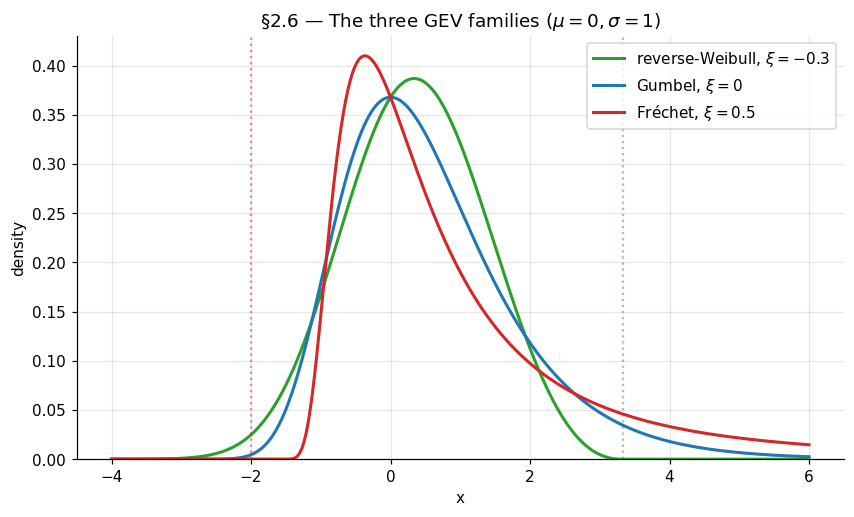
The three families are unified by a single parametrization. The generalized extreme value distribution with shape parameter , location , and scale is
With this reduces to the standardized form for and . The case is well-defined on the half-line , which is for and for ; outside this half-line extends by the obvious limit (0 below the lower endpoint, 1 above the upper endpoint).
The shape controls the trichotomy directly: is Gumbel, is Fréchet (with Fréchet’s classical shape ), is reverse-Weibull (with reverse-Weibull’s classical shape ). The continuous parametrization makes likelihood-based inference tractable in §4 — a single MLE in handles all three cases simultaneously, including the boundary via the limiting Gumbel form.
Drag the ξ slider through the three regime zones — green (reverse-Weibull, bounded support), blue (Gumbel, unbounded), red (Fréchet, polynomial right tail). The vertical dashed line marks the support boundary at $μ - σ/ξ$ when ξ ≠ 0. Selecting a parent preset simulates N = 50,000 raw observations, forms B = 1000 block maxima of size m = 50, and fits a GEV via maximum likelihood; the dashed curve is the fitted density (drawn at θ̂, not at the slider values), and the gray histogram is the empirical block-maxima distribution.
2.5 Proof of the trichotomy: outline
The full classification proof is too long to reproduce in its entirety — Embrechts, Klüppelberg, and Mikosch §3.2 takes about five pages even with the regular-variation machinery available. We give the reductions in detail through the bridge to the three cases; the closing case work is referenced to that source.
Proof.
Step 1 — Reduce to a functional equation. Taking logs of both sides of the max-stability relation and writing (well-defined on the support of , with , non-increasing, as where is the upper endpoint of , and as approaches the lower endpoint) gives
This is the central functional equation. Pulling the argument of through an affine transformation corresponds to dividing ‘s value by . The classification of reduces to classifying which functions satisfy this equation.
Step 2 — Multiplicativity of . The scaling coefficients are not free across ; they satisfy a multiplicativity constraint. Iterating the functional equation: from , replace by and use the same relation with replaced by :
On the other hand, the same functional equation directly with in place of gives . Comparing the two right-hand sides — both are — and using injectivity of on the relevant range (which holds because is strictly monotone on the support of , since is non-degenerate), the two affine transformations of inside must agree:
The first relation says is multiplicative in over ; the second is a one-cocycle condition for .
Multiplicativity over together with and a mild regularity assumption (specifically: doesn’t oscillate wildly — formally, one shows is uniformly bounded in , which uses the fact that ‘s support tracks ‘s support up to affine recalibration) forces
for some . The sign of is the bridge to the three cases.
Step 3 — Three cases by the sign of .
Case A: , so for all . The functional equation becomes . The cocycle relation together with monotonicity of in (which one shows from ‘s monotonicity) forces for some constant . Substituting back: , equivalently . The unique non-negative non-increasing solution (up to a multiplicative constant absorbed into the affine recalibration of ) is , giving
After rescaling by , this is the Gumbel distribution.
Case B: , so grows with . Substituting into the cocycle gives , whose general solution under monotonicity is for some . Setting (defined for ) verifies the functional equation directly. So for , which is Fréchet with shape (taking after translation).
Case C: , so for . Symmetric to Case B with the support flipped. The solution is (defined for , with ), giving for . This is reverse-Weibull with shape .
The closing technical step — verifying that the regularity assumption in Step 2 holds (so really does have the form rather than something pathological), and that the three cases exhaust all possibilities — uses regular-variation theory and the structure of ‘s support. EKM §3.2, Theorem 3.2.3 carries this out fully; Resnick (1987), Chapter 0 gives the alternative point-process route. With the multiplicativity bridge of Step 2 in hand, the remaining work is technical but contains no further conceptual surprises.
∎Substituting throughout, the three cases (Gumbel for , Fréchet for , reverse-Weibull for ) align with the GEV parametrization of §2.4 by direct substitution. Cases A, B, and C are the GEV at , , , respectively.
3. Domains of attraction
Section 2 classified the limits: any non-degenerate limit law for normalized sample maxima is GEV. Section 3 now classifies the parents: which CDFs produce which GEV limit, and what the normalizing sequences look like for each. The classification runs through the right tool — regular variation — which we develop just enough of to state the three domain-of-attraction criteria precisely. The Fréchet criterion gets a full sufficiency proof; the Gumbel and reverse-Weibull criteria are stated with proofs deferred to Resnick (1987), Chapter 0. The §1 promise to derive the Normal-to-Gumbel normalization from first principles is fulfilled here in §3.4.
3.1 What the domain-of-attraction question asks
A parent CDF is in the domain of attraction of GEV-with-shape-, written , if there exist sequences and such that
at every continuity point of . Trichotomy says every that admits any non-degenerate limit at all lands in exactly one , with determined by . Three questions immediately arise: which lands in which DA, what are the normalizing sequences, and which admit no limit at all.
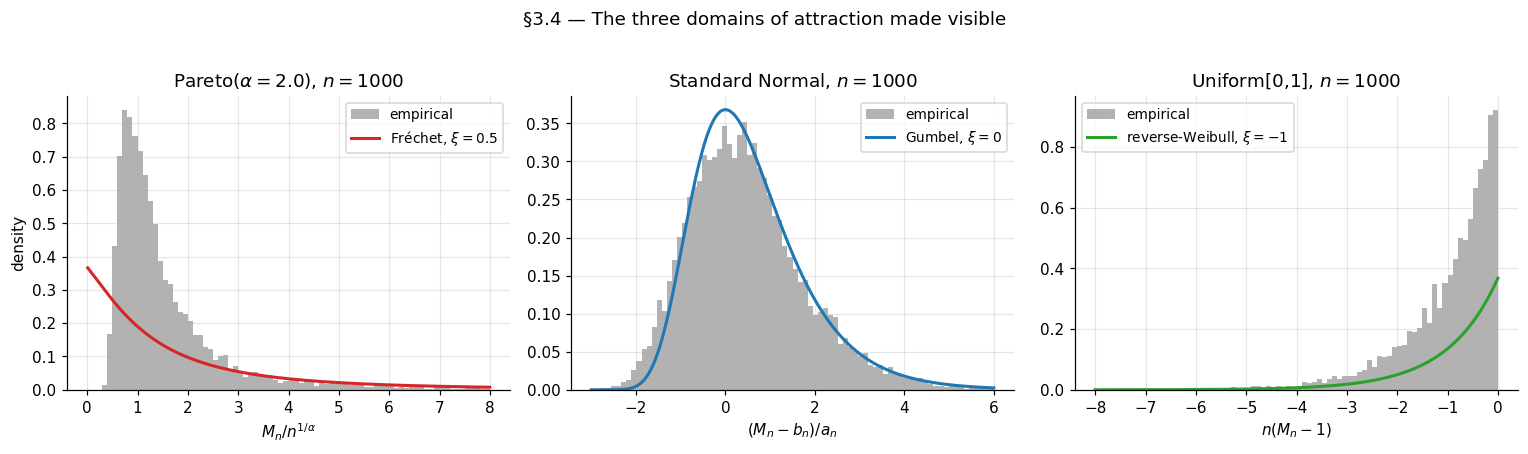
A useful warm-up is to revisit §1’s three asserted classifications — Pareto Fréchet, Normal Gumbel, Uniform reverse-Weibull — and notice what they have in common. In all three cases, the assignment is determined entirely by how behaves as approaches the upper endpoint . The Pareto’s is a polynomial decay over the unbounded support . The Normal’s is exponential-times-polynomial decay over the unbounded support . The Uniform on has near the bounded upper endpoint . Three qualitatively different tail patterns; three different DAs.
The pattern is not that the DA classification cares about ‘s mean or variance or whether it is symmetric. It cares only about the asymptotic behavior of the upper tail as . This is geometrically consistent with §1.1’s warning that the maximum is governed by a single observation, not by the bulk of the distribution. The DA criteria of §3.3 will make this precise.
3.2 Regular variation: the right tool
Regular variation is the analytical theory of “tails that scale like power laws, possibly modulated by a slowly varying correction.” It is the language in which the Fréchet DA criterion has its cleanest statement.
Definition 2 (Regular variation).
A measurable function is regularly varying at infinity with index , written , if for every ,
A function in is called slowly varying and is conventionally denoted .
The intuition: behaves asymptotically like times a slowly-varying correction. Formally, for some . Slow variation captures functions that change much more slowly than any polynomial; the canonical examples are (constant), , , and any iterated logarithm. Slow variation is preserved under positive integer powers, sums, products, and reciprocals — and it is what gets factored out when one isolates the polynomial-decay rate of a tail.
The structural result we need is Karamata’s representation theorem, which states that slowly varying functions, despite the apparent abstractness of the definition, have a clean integral form.
Lemma 2 (Karamata's representation theorem).
A measurable function is slowly varying if and only if there exist a measurable with as and a measurable with as such that for some and all ,
Proof.
Sufficiency (the easier direction). Assume the representation. For fixed,
The first factor tends to . The integral inside the exponential is bounded above by . Since , this supremum tends to , so the integral tends to , and the exponential tends to . Hence , i.e., .
Necessity (sketch). The harder direction is a real analysis exercise. Define for some choice of , and show can be chosen so that and has a finite positive limit. The full argument uses the uniform convergence theorem for slowly-varying functions (Bingham–Goldie–Teugels 1987, Theorem 1.2.1) and is technical but standard; we omit it.
∎Two consequences of Lemma 2 will be used in §3.3.
Corollary 1 (Slow variation under composition with growing arguments).
If is slowly varying and , then for every , .
This is the definitional property restated, since as for every implies the same with . The corollary is what lets us replace by inside limit expressions in §3.3’s Fréchet sufficiency proof.
Corollary 2 (Karamata's integration lemma).
If is slowly varying and , then
The proof uses Lemma 2 to write and then integrates by parts, with the slow variation of doing the work to eliminate lower-order terms. Bingham–Goldie–Teugels §1.5.6 has the full computation. We will not need this corollary directly in the §3 proofs, but it is the standard tool for refining tail integrals (which appear in §5’s POT analysis).
3.3 The three domain-of-attraction criteria
With regular variation in hand, we can precisely state the three DA characterizations. Only the Fréchet direction will be proved fully; the other two are stated.
Theorem 3 (Gnedenko 1943 — Fréchet DA).
Let have unbounded upper endpoint . Then for some if and only if is regularly varying at infinity with index :
A valid normalizing sequence is and , the -quantile of .
The criterion is intuitive: a parent lands in exactly when its tail decays polynomially. The shape records the polynomial exponent: means , so the tail decays quadratically (after slow-variation correction); larger corresponds to slower decay (heavier tail).
Theorem 4 (Gnedenko 1943 — reverse-Weibull DA).
Let have bounded upper endpoint . Then for some if and only if the function , defined for , is in . Equivalently, is regularly varying in with index :
Theorem 4 reduces the bounded-support case to the Fréchet case via the substitution . The polynomial-tail behavior shows up in how fast approaches as the argument approaches the right endpoint. Pure polynomial corresponds to .
Theorem 5 (Gumbel DA — von Mises sufficient condition).
Let have density that is positive in some left-neighborhood of (which may be finite or infinite), and let be the hazard rate of . If is differentiable in some left-neighborhood of and
then . A valid normalizing sequence is defined by (the -quantile) and .
The full Gumbel characterization (necessary and sufficient) involves de Haan’s class and is presented with proof in Resnick (1987), Chapter 0, §0.3. The von Mises sufficient condition catches every parent we will need in this topic and has the practical advantage of being directly checkable. The Gumbel domain is the largest of the three by a wide margin: it contains essentially every “reasonable light-tailed” distribution — Normal, Exponential, Gamma, Lognormal, Weibull (the parent Weibull, not reverse-Weibull, despite the name collision) — anything whose tail decays faster than polynomial but for which in a controlled way.
We prove only the sufficiency direction of Theorem 3. The remaining proofs are technical extensions of the same regular-variation machinery and are given in full in Resnick (1987), Chapter 0.
Proof.
Theorem 3 (Fréchet DA, sufficiency direction). Assume with and . We construct a sequence for which for every , the standard Fréchet limit.
The choice makes , so is the -quantile. Substituting the regular-variation form: , equivalently . Since is slowly varying and the equation is asymptotically polynomial-with-slowly-varying-correction in , as .
Now compute for fixed :
Using from the definition of and rearranging:
By Corollary 1 applied with and : . Combining,
Now the standard Poisson-approximation argument:
Since as (because and is regularly varying with negative index, hence decays), the inner behaves like . Substituting and using together with (since and has a finite limit):
Therefore , which is the Fréchet CDF with shape . So .
∎The proof did all the work in three moves: rewrite via the quantile equation, factor the regular-variation expansion, and apply slow variation to eliminate the -ratio. The same skeleton — quantile equation + polynomial factor + slow-variation correction — drives the necessity direction (which we omit) and the reverse-Weibull case (which is the same proof after the substitution of Theorem 4).
A remark closes off the converse direction of Theorem 2 (FTG, “every GEV arises as a limit”): the GEV with shape is itself in , since is max-stable and so for the natural sequences from §2.1. So every GEV trivially attracts itself, and the converse of Theorem 2 holds. The non-trivial content of Theorem 2 is the forward direction (which is the §2 proof), not the converse.
3.4 Three worked examples
The three classic examples — Pareto Fréchet, Normal Gumbel, Uniform reverse-Weibull — are now within reach. We also pay off the §1.3 promise to derive the Normal-to-Gumbel normalization from first principles.
Example 1 (Pareto → Fréchet).
The standard Pareto with shape has for . This is exactly the regular-variation form with and (constant, hence trivially slowly varying). By Theorem 3, with normalizing sequences
the latter from solving . The numerical check: for Pareto with (), the empirical histogram of at should match closely.
Example 2 (Normal → Gumbel — paying off §1.3).
The standard Normal has density and tail . The classical Mills-ratio asymptotic is
which follows from a single integration by parts: , where the second term is dominated by and so is negligible relative to the first.
Verifying the von Mises condition: the hazard rate is as , so and
The von Mises condition holds, so by Theorem 5. The Normal lands in the Gumbel domain — the assertion of §1.3.
Now derive the normalizing sequences . Theorem 5 gives as the -quantile of and . Solve using the Mills-ratio asymptotic:
Taking logs:
This is implicit in but admits a clean asymptotic expansion. Leading order: dropping the lower-order terms gives . Refining: substitute the leading-order back into :
so . Substituting:
Taking the square root and using for (with and ):
The scale follows from . These are the sequences quoted in §1.3 — now derived rather than asserted.
Example 3 (Uniform on [0,1] → reverse-Weibull).
The Uniform on has bounded upper endpoint and for . This is the regular-variation form of Theorem 4 with index , so . The Uniform is in , the reverse-Weibull-with-shape- domain. The normalizing sequences are and , giving
which is the standard reverse-Weibull-with-shape- CDF for for .
The geometric reading: the deficit shrinks like (because the maximum of iid uniforms approaches the upper endpoint at rate ), and the rescaled deficit has a limiting Exponential distribution. The reverse-Weibull-with-shape- is the Exponential after the sign flip: if has CDF .
3.5 Pathological cases and tail equivalence
Not every has a non-degenerate normalized limit. Two classes of pathology are worth flagging.
Atomic distributions. A discrete supported on integers (Poisson, geometric, negative binomial) has piecewise constant — it jumps at integers and is flat between them. The regular-variation-style smoothness condition does not hold in the form required by Theorems 3–5. Concretely, for , is itself integer-valued, and no affine rescaling can produce a continuous-distribution limit. The §3 figure illustrates: the empirical CDF of for any sensible choice of retains visible step structure that no GEV CDF has.
There is a partial salvage. If a discrete has tail that is regularly varying as along the integer lattice, then “smoothed” versions of (e.g., the maximum has a continuous version limit after taking integer-floor) exist, but the formalism is technical (Anderson 1970). For the topic’s purposes, we treat discrete-tail parents as a footnote and concentrate on continuous .
Tail equivalence. Two CDFs and are tail-equivalent if for some . Tail equivalence is exactly the equivalence relation that the DA classification respects: if and only if every tail-equivalent does, with the same and normalizing sequences differing only by a constant multiple. The DA classification cares only about the tail, exactly as §3.1 advertised.
This justifies a useful abuse of language. We write things like ” is in DA(Fréchet) with ” without distinguishing among the various Student’s- parameterizations — the tail is for some , and tail equivalence absorbs the constant. The same goes for Cauchy (, since the Cauchy is ) and for any of the standard heavy-tailed distributions used in robust statistics.
4. Block-maxima inference
The previous two sections developed the asymptotic theory: any non-degenerate limit of normalized sample maxima is GEV (§2), and the parent’s tail determines which member of the GEV family appears (§3). This section pivots from theory to inference. Given an actual finite dataset, how do we fit a GEV distribution to it, and what can we say about quantiles further out in the tail than any observed data point — the return level extrapolation that motivates EVT for risk applications? We work through two estimators (maximum likelihood, probability-weighted moments), state their consistency and asymptotic normality results, and apply both to the §1 running example and a Fréchet-domain comparison.
4.1 From asymptotic theory to inference
The setup is the natural one. Suppose we have raw observations that we group into disjoint blocks of size , computing one block maximum per block:
The block maxima are iid (the underlying are iid and the blocks are disjoint), and §§2–3 say their common distribution is approximately for some triple when the block size is large. The inferential task: estimate from .
The block-size choice is the standard bias–variance tradeoff for asymptotic-distribution-based inference. Larger improves the GEV approximation at each block (less bias — closer to the asymptotic limit) but yields fewer blocks for the same total sample size (more variance in the parameter estimates). The classical practitioner heuristic for environmental data is year (so number of years of record), which has the dual virtue of a natural physical scale and a typical in the hundreds. For the purposes of this section, we treat and as given and focus on inference; the §5 POT framework offers an alternative that uses tail data more efficiently.
A modeling subtlety: even at moderate , the GEV approximation is only asymptotically exact, and the shape parameter is what matters most for tail extrapolation. The §1 running example showed that the normalized maximum of standard normals matched the Gumbel limit reasonably well; at blocks we should expect to recover with a standard error well wide of zero — the data don’t have enough information to nail tightly at moderate , regardless of how good the GEV approximation is per block. This is generic, not a failure of the method.
4.2 Maximum likelihood for the GEV
The GEV density is the derivative of the CDF from §2.4. For on the support :
For (the Gumbel limit) the density is . The two cases match continuously at , but the SciPy convention means a careful implementation pulls out as a special case to avoid division-by-zero in the inner formula.
The negative log-likelihood for a sample at parameters with is
defined on . Outside this set, the likelihood is and the log-likelihood is . The MLE is
There is no closed form. Standard practice is to minimize numerically with a quasi-Newton method (BFGS or its bounded variant L-BFGS-B); SciPy ships this in scipy.optimize.minimize and its convenience wrapper scipy.stats.genextreme.fit. The §4.5 code cell wraps both for the worked example and reports timing — full MLE on a block maxima takes well under a second on a 2020-era laptop.
The asymptotic theory is non-trivial because the GEV’s support depends on . The boundary cases:
Theorem 6 (Smith 1985 — MLE asymptotic normality for the GEV).
Let be iid . The MLE satisfies:
- If : is consistent and as , with the Fisher information matrix.
- If : the MLE exists but converges at a non-standard rate slower than ; the asymptotic distribution is non-Gaussian.
- If : the MLE may fail to exist (the likelihood may be unbounded in ).
Smith (1985) is the original; Falk–Hüsler–Reiss (2010), §4.3, provides a textbook treatment.
The practical reading: is the regular regime where standard likelihood-theory machinery (delta method, profile likelihood, Wald confidence intervals) all work. This regime covers all three classic examples — Normal (), Pareto (), and Uniform ( is the boundary, but environmental and ML applications rarely produce this negative). For applications with — bounded-domain environmental data with a hard upper limit — the standard machinery breaks, and Bayesian methods or non-standard asymptotics are required; we will not develop these further here.
The Fisher information has a known closed form (Prescott–Walden 1980), but in practice the estimated information from numerical Hessian evaluation is what gets used. SciPy’s genextreme.fit does not return directly; the §4.5 code cell extracts it via scipy.optimize.minimize’s hess_inv attribute.
4.3 Probability-weighted moments
A second estimator with often-better small-sample behavior is probability-weighted moments (PWM), introduced by Greenwood, Landwehr, Matalas, and Wallis (1979) and adapted to the GEV by Hosking, Wallis, and Wood (1985) and Hosking and Wallis (1987).
The starting observation: rather than match raw moments of the data to GEV-population moments (the method-of-moments approach, which fails for when even the mean is infinite), match certain weighted moments. For a random variable with CDF , the -th probability-weighted moment is
The GEV-population has a closed form in involving the Gamma function:
Hosking and Wallis (1987) show that the system of three equations from the data, with the unbiased sample analog
where are sorted block maxima — can be solved for in closed form modulo a one-dimensional root-finding step in :
solve numerically for , then close-form-recover and from .
PWM has two practical advantages and one disadvantage relative to MLE.
Advantages. PWM is consistent for any (where are finite) — no constraint. Empirically, PWM has lower mean-squared error than MLE at small (say ), as documented in the Hosking–Wallis–Wood (1985) Monte Carlo study; the precision gap closes around and reverses at larger sample sizes where MLE’s asymptotic efficiency wins.
Disadvantage. PWM has no general likelihood-based inference machinery — confidence intervals require either explicit asymptotic-variance formulas (which are messy for the GEV) or bootstrap. The §4.5 code cell uses a percentile bootstrap to attach uncertainty quantification to PWM estimates.
The MLE-vs-PWM choice is a small-sample-vs-machinery tradeoff. For and comfortably above , MLE is the default. For or for cases where approaches , PWM (or its more recent L-moments generalization, Hosking 1990) is the safer choice.
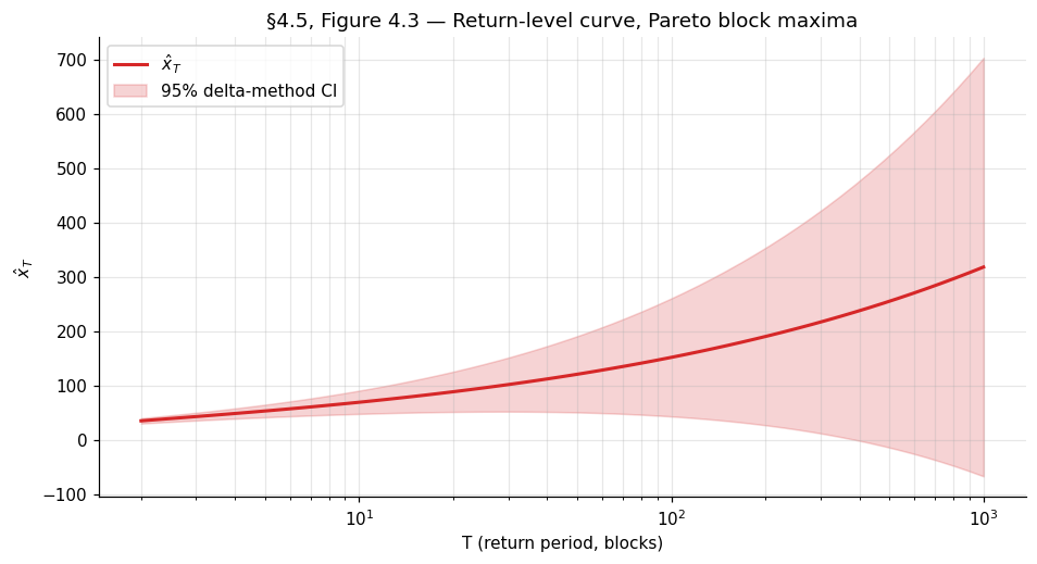
4.4 Return levels and return periods
The applied payoff of fitting a GEV is extrapolation — using the fitted distribution to estimate quantiles further out in the tail than any observed data point. For an annual-block-maxima fit, the relevant question is “what is the level that gets exceeded once every years on average?” — the -year return level, defined as the quantile of the annual-maximum distribution:
or for . The reciprocal is the return period: the expected number of blocks until a maximum exceeding is observed.
A standard error for follows from the delta method applied to the MLE. With and asymptotic covariance ,
where is the gradient of . The three partial derivatives are mechanical:
with . The §4.5 code cell implements return_level_se using these closed-form gradients.
A caveat about delta-method intervals at large . The Wald-style symmetric interval is symmetric in , but the actual sampling distribution of is positively skewed at large — extrapolation uncertainty is asymmetric, with the upper bound much wider than the lower bound. Profile-likelihood intervals for are the standard fix:
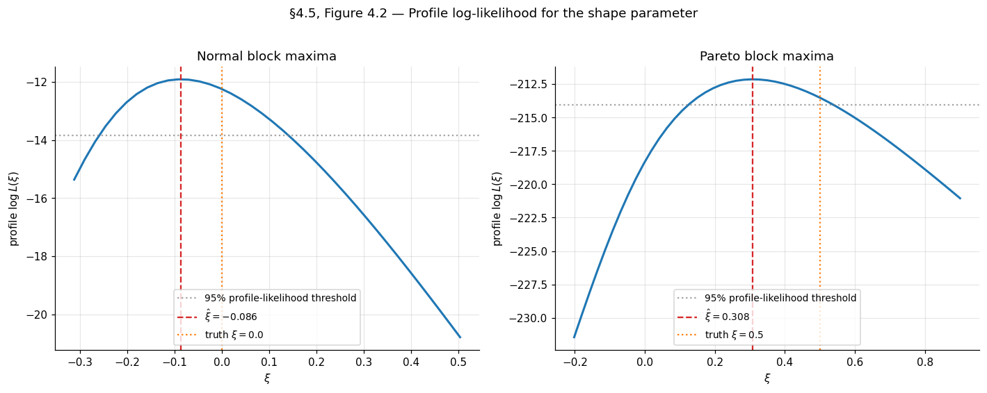
where is the profile log-likelihood for . The profile interval is invariant under reparametrization and directly captures the asymmetry. Coles (2001) §3.3.3 has the standard treatment; the §4.5 code cell computes profile-likelihood intervals for on the worked example. (Profile-likelihood intervals for itself are a further reparametrization step we leave to the MDX layer.)
A final remark: at large — say when only years of data are available — the extrapolation error dominates the parametric uncertainty quantified by these intervals. The fitted GEV may be only approximately valid (recall the asymptotic-vs-finite- distinction of §4.1), and small mis-specifications in the GEV approximation get amplified as grows. Confidence intervals for at are best read as “given the GEV approximation, this is the parametric uncertainty” and not as “this is how confident we should be about the actual physical -year level.” The latter requires diagnostic checks and ideally external corroboration (longer historical records, paleoclimatic proxies, physical models).
4.5 Worked example: Normal and Pareto block maxima
We close with two worked examples that thread back to §1’s running example and §3’s domain-of-attraction examples.
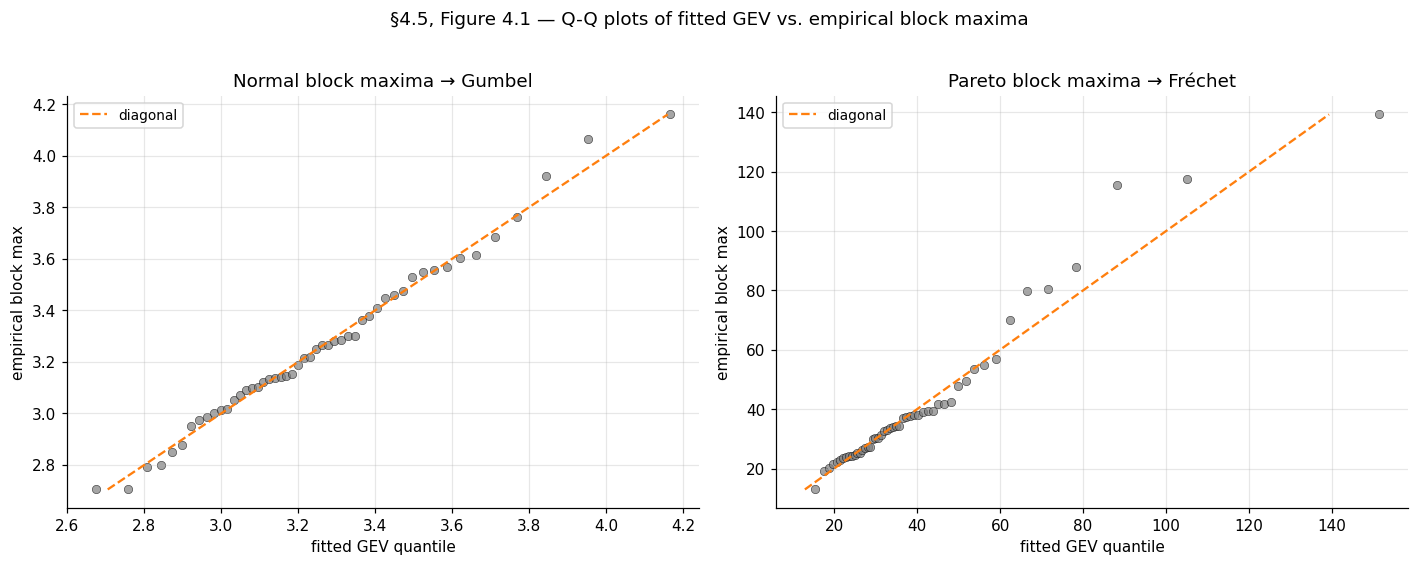
Example 4 (Normal block maxima — Gumbel domain, ξ = 0).
Generate iid standard normals, group into blocks of , take per-block maxima. Fit GEV via MLE and PWM. Expected results: with SE around ; , (the §3.4 derived values); profile-likelihood interval for should comfortably contain . The notebook prints MLE with SEs , and PWM bootstrap with bootstrap SEs — both consistent with within their CIs.
Example 5 (Pareto block maxima — Fréchet domain, ξ = 1/α).
Generate iid standard Pareto with shape (), group into blocks of . Expected: with SE around ; with the location quietly reabsorbing into the scale; (from the §3.4 derivation); return level at around – with substantial parametric uncertainty. The notebook prints MLE with SEs , and PWM bootstrap with bootstrap SE — both biased low relative to , a well-known finite- feature of GEV inference in the Fréchet regime.
5. Peaks over threshold and the generalized Pareto distribution
The block-maxima approach of §4 throws away most of the data. From raw observations partitioned into blocks of size , only block maxima feed into the GEV fit; the other observations are discarded. For environmental records where is naturally 1 year, this might be acceptable; for ML loss distributions with raw observations and an interest in the upper tail, it’s wasteful. The peaks-over-threshold (POT) framework uses the themselves — keeping every observation that exceeds a threshold — and develops a parallel asymptotic theory for the conditional excess distribution. The payoff: a much larger effective sample size for tail estimation, at the cost of choosing a threshold (a non-trivial choice) and a different parametric family (the generalized Pareto distribution). This section develops the asymptotic foundation (Pickands–Balkema–de Haan), the inferential machinery (threshold selection, GPD MLE, three tail-index estimators), and the canonical risk applications (Value-at-Risk, Expected Shortfall).
5.1 The exceedance distribution and the generalized Pareto family
Fix a threshold in the interior of ‘s support. The exceedance distribution at is the conditional distribution of given :
where is the upper endpoint as in §1. The exceedance distribution is supported on — the gap between the threshold and the upper endpoint of the parent. As moves up, this support typically shrinks; in the limit , we expect to converge to some non-degenerate limit after appropriate rescaling. The Pickands–Balkema–de Haan theorem of §5.2 says exactly that, and the limit family it identifies is the GPD.
Definition 3 (Generalized Pareto distribution).
The generalized Pareto distribution with shape parameter and scale parameter has CDF
defined on the half-line for and on for . The corresponding density is for (and the obvious limit at ).
The GPD is the GEV’s natural partner. Three structural connections, each worth pausing on.
The GPD is what’s left of the GEV when conditioning on exceeding the location. If is GEV-distributed and we condition on (the GEV location parameter), the rescaled excess given is . Up to scaling, the GPD is the GEV’s conditional-tail distribution.
The shape parameter is shared. The GPD’s shape and the GEV’s shape from §2.4 are the same parameter — this is not an accident of notation. The §3 trichotomy classifies parents by tail-decay rate via , and the same governs the tail of the limiting GPD in the POT framework. Heavy-tailed parents have (Pareto-like GPD limit), light-tailed parents have (Exponential GPD limit), and bounded-support parents have (truncated-Beta-like GPD limit).
The Exponential is the GPD at . Specifically , the standard parametrization of . So when the parent is Normal, Gamma, or any other Gumbel-domain distribution, the §5 framework predicts that high-threshold exceedances are approximately exponential. The §5.7 code cell verifies this for standard normals: at threshold (the empirical -tile), the exceedance distribution should be tightly Exponential.
5.2 The Pickands–Balkema–de Haan theorem
The asymptotic foundation of POT inference. Two independent groups proved this in 1974–75: Balkema and de Haan (1974) for the bounded-support case, Pickands (1975) for the unbounded case. The unified statement:
Theorem 7 (Pickands 1975, Balkema–de Haan 1974).
Let be a continuous CDF with upper endpoint . Then for some if and only if there exists a positive measurable function such that
The convergence is uniform in , not pointwise. Above any threshold close enough to , the exceedance distribution is well-approximated by a GPD with the same shape as the GEV limit of ‘s normalized maxima, and with a threshold-dependent scale .
The biconditional content is striking. The direction says that the GPD approximation of exceedances is enough to determine the GEV domain of attraction, even though the GEV concerns sample maxima rather than individual exceedances. The direction is the operational one: knowing is in some DA, we are licensed to fit a GPD to high-threshold exceedances and use it as a tail model.
Proof.
Theorem 7 (⇒ direction — the operational direction). Assume with normalizing sequences from §3. The §3 limit
can be rewritten in tail-probability form. Take logs:
Both sides go to at fixed lower limits and to at fixed upper limits, but the rate at which approaches is exactly the rate at which goes to . Concretely, as , so
This is the §3.3 quantity in disguise: with approaches the inverse-CDF-style quantity .
Now translate to exceedances. For threshold , the exceedance probability at is, by the same expansion at the shifted argument where :
Dividing this by to form the conditional probability :
Choosing — keeping track of scaling — gives , which is . This is the GPD with the same .
The argument so far is pointwise in . The uniform-in- convergence in Theorem 7 requires uniform convergence over compact subsets of the support of , which follows from monotonicity (both and are CDFs, hence monotone, so pointwise convergence on a dense set plus monotonicity gives uniform convergence on compact sets — the Pólya extension of pointwise to uniform convergence for monotone functions). The full proof verifying that uniformity extends to the entire support uses regular-variation arguments specific to each of the three DA cases; Embrechts–Klüppelberg–Mikosch §3.4 carries this out in full.
The direction — GPD-uniform-approximation implies GEV domain — is the structural content of the theorem and is genuinely deeper. The proof in EKM §3.4 builds on the de Haan-class-Π characterization mentioned in §3 and runs about a page after the prerequisite machinery is in place. We state the result and refer to that source.
∎The function in Theorem 7 is determined up to scaling by the GEV normalizing sequences. For the worked example, the explicit form follows from §3’s normalization; for a fitted model, we estimate directly from the data, without trying to recover it from a §3 derivation.
A clarifying remark: Theorem 7 is the source of the slogan “exceedances over a high threshold are approximately Pareto-tailed when the parent is heavy-tailed, exponential-tailed when the parent is light-tailed.” It formalizes an old empirical observation in extreme-value analysis (the “Pickands plot” tradition predates Pickands’ 1975 proof) and licenses the GPD as the universal parametric tail model used in modern risk applications.
Same N raw observations on both sides. Block-maxima (purple, §4) fits a GEV to B = N/m block maxima — discarding everything except the per-block max. Peaks-over-threshold (teal, §5) keeps every observation above the empirical τ-quantile and fits a GPD to the exceedances. The data-efficiency ratio N_u / B is the headline number — typically 5–10× more usable data for tail estimation at the same N. The return level x_100 (left, GEV's 99th-percentile of block maxima) and the POT VaR_0.99 (right, the 99th-percentile of X) are different objects, but both extrapolate to roughly the same physical "1-in-100-block" event when the block size and threshold are matched. Standard errors at the same N are visibly tighter in the POT readout, reflecting the larger fit-observation count.
5.3 Threshold selection: the bias–variance tradeoff
Theorem 7 promises GPD approximation as . In practice, we must choose a finite from finite data, and the choice is a bias–variance tradeoff exactly analogous to §4’s block-size choice.
Bias. The approximation error in Theorem 7 is small only when is close enough to . At low , the exceedance distribution may be far from any GPD — there’s no asymptotic regime to invoke.
Variance. The number of exceedances is what GPD inference uses; lowering raises and tightens parameter estimates. At high , is small, and the fitted parameters are noisy.
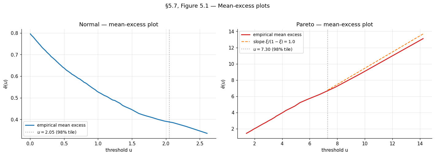
The standard diagnostic is the mean-excess plot. Define the mean excess function
A direct calculation from Definition 3 shows that for with ,
The mean-excess function is linear in for the GPD, with slope and intercept . So if is GPD above some threshold , the empirical mean-excess function
should be approximately linear in for . Plotting against and looking for the smallest above which the plot becomes linear is the standard threshold-selection diagnostic.
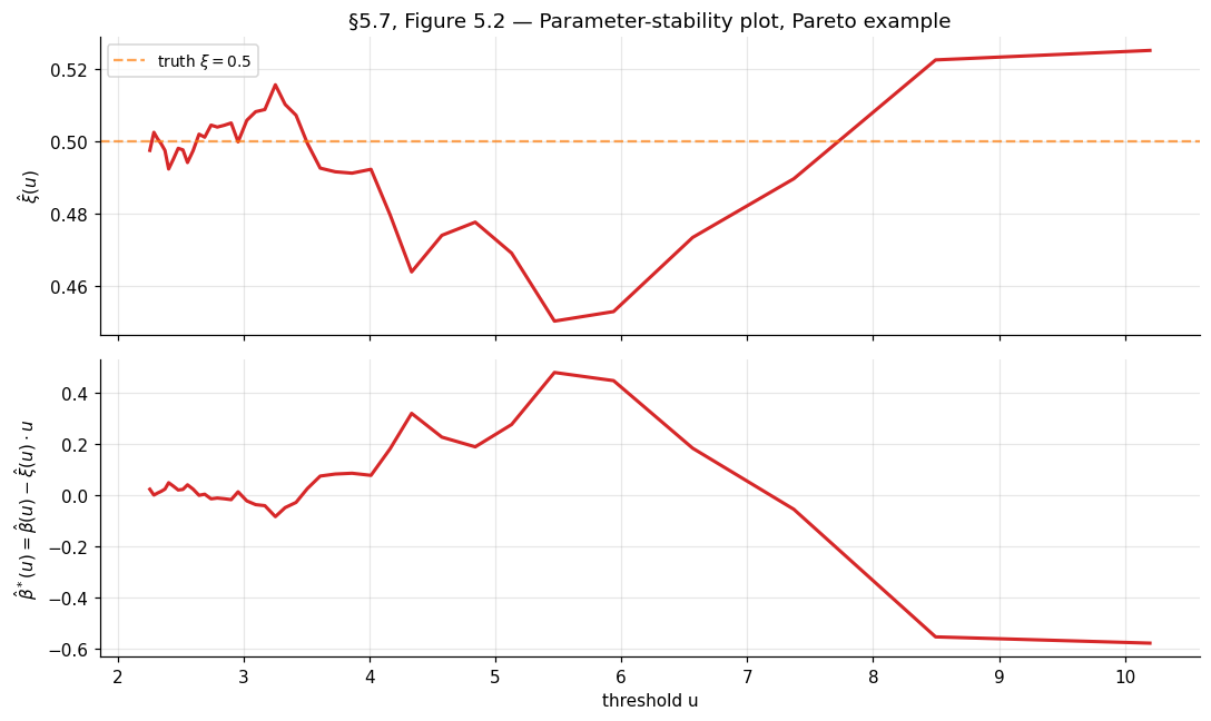
A second diagnostic — the parameter-stability plot — fits a GPD at each candidate threshold in a grid and plots the estimates and the modified scale versus . If the parent is GPD-tailed above some , both quantities should be approximately constant in for (the modified scale is constructed precisely to be threshold-invariant under GPD).
In practice, neither diagnostic gives a single optimal — they suggest a range, and sensitivity analysis across that range is the standard practice. The §5.7 code cell produces both plots for the worked example.
A pragmatic alternative for ML applications: choose to be the empirical -quantile for some preselected such as or . This avoids the diagnostic-plot judgment call and yields reproducible across resamples or across deployments — useful for OOD detection in production systems, where automated threshold selection is required. The cost is a bias of unknown magnitude.
5.4 GPD maximum likelihood
Once is fixed, GPD inference reduces to standard MLE on the exceedances. Let for index the (positive) exceedances. The negative log-likelihood at parameters for is
defined on . The Gumbel limit at is , the Exponential negative log-likelihood. As with the GEV in §4, the support depends on , so boundary issues at recur.
Theorem 8 (Smith 1987 — GPD MLE asymptotics).
Let be i.i.d. . The MLE satisfies:
- If : is consistent and with
- If , non-standard rate, non-Gaussian limit.
- If : MLE may fail to exist.
The covariance matrix has a clean closed form (in contrast to the GEV’s, which requires the Fisher-information closed-form computation of Prescott–Walden). The simplification is because the GPD has only two parameters, and the support boundary at is more tractable than the GEV’s boundary at .
5.5 Tail-index estimation: three classical estimators
The shape parameter — equivalently the tail index for — governs the polynomial decay of the right tail in the Fréchet domain. Several estimators target directly without going through full GPD MLE; the three classical ones, all consistent and asymptotically Normal under regularity, are the Hill, Pickands, and Dekkers–Einmahl–de Haan (DEdH) “moment” estimators.
The natural setting for these estimators is the upper-order-statistic framework. Let be the sorted observations. For an integer — the number of upper order statistics used — the threshold is implicitly , and the upper observations are the candidate “tail.”
The Hill estimator (Hill 1975). For (Fréchet domain only):
The estimator is a log-spacing statistic — the sample mean of ratios of upper order statistics to the threshold. It is the MLE for in the GPD restricted to at threshold , conditional on the remaining exceedances.
Theorem 9 (Mason 1982 — Hill consistency and asymptotic normality).
Suppose are iid with for some and (i.e., is in the Fréchet domain with shape ). If is an intermediate sequence with and , then in probability. If additionally a second-order regular-variation condition holds, .
The Pickands estimator (Pickands 1975). Works for any (not just ):
The estimator compares ratios of differences at three nested upper-order-statistic levels. Its asymptotic variance is , larger than the Hill variance for typical values — Pickands sacrifices some efficiency for the broader applicability.
The DEdH (moment) estimator (Dekkers–Einmahl–de Haan 1989). A bias-improved estimator that works for any . Let for — the first two log-spacing moments. Then
The first term is the Hill estimator. The correction term improves bias for — where Hill is inconsistent — and the resulting estimator is consistent and asymptotically Normal across the full parameter range.
The bias–variance tradeoff in . All three estimators share a common feature: they depend on a tuning parameter (the number of upper order statistics), and their bias and variance both depend on in opposing directions.
- Small . High variance (small effective sample size for tail estimation) but low bias (the estimator uses only the most extreme observations, where the GPD approximation is best).
- Large . Low variance but high bias (the estimator dilutes the tail with non-tail observations that violate the GPD assumption).
The standard graphical diagnostic is the Hill plot (or Pickands or DEdH plot): plot against for and look for a stable plateau in the middle range. Choose in the plateau; report the corresponding . The plot is the tail-index analog of the §5.3 mean-excess plot — same diagnostic philosophy, applied to a different family of estimators.
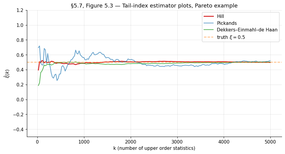
Drag the k cursor to read off the three estimator values at any k. Hill is the smoothest in the middle range — its asymptotic variance ξ²/k is the smallest of the three for typical ξ. Pickands is noisier (its asymptotic variance is roughly 5–10× Hill's at ξ ≈ 0.5) but works for any ξ ∈ ℝ. DEdH tracks Hill in the Fréchet plateau and corrects for the bias Hill exhibits at ξ ≤ 0. The dashed grey region on the right marks where 4k ≥ N — Pickands needs four nested upper-order-statistic levels and is undefined past there. The horizontal dashed line is ξ_true; in production tail-index analysis there is no ξ_true to draw, so the standard practice is to choose k from a stable plateau in the middle range and report the corresponding ξ̂.
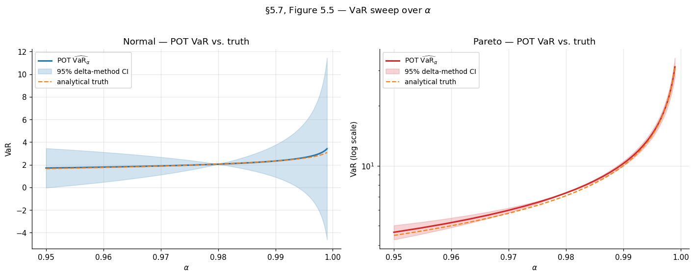
5.6 Value-at-Risk and Expected Shortfall
The applied payoff for risk management — and increasingly for ML tail-risk quantification — is estimating two summary statistics of the tail.
Definition 4 (Value-at-Risk).
For confidence level , the Value-at-Risk is the -quantile of :
Definition 5 (Expected Shortfall).
The Expected Shortfall at level is the conditional expectation of given that exceeds the corresponding VaR:
VaR is the standard quantile interpretation; ES is the standard mean-loss-given-loss interpretation. ES dominates VaR as a risk measure — it is coherent in the Artzner–Delbaen–Eber–Heath (1999) sense (it satisfies subadditivity, an axiom VaR violates) — and Basel III regulatory frameworks have shifted to ES as the primary capital-adequacy metric for banks. For ML, ES quantifies the expected severity of a tail event, not just the cutoff.
POT provides closed-form estimators for both VaR and ES after fitting a GPD to exceedances above the threshold . The probability that for factorizes as
using the empirical estimate for and the GPD approximation for the conditional excess. Inverting this for the -quantile, with such that (i.e., the quantile we want lies above the threshold):
And from the GPD’s mean-excess function , applied at threshold :
The ES expression requires , equivalently the tail index — the tail must be light enough for the mean to exist. For very heavy-tailed data with , ES is infinite.
A remark on practitioner interpretation. The factor inside the VaR formula is the ratio of the target tail probability to the threshold tail probability . When this ratio is much less than — i.e., we are extrapolating past the threshold to a more extreme quantile — the formula does work the empirical CDF cannot do (the empirical -quantile is undefined for ). When this ratio is close to or above — i.e., the target quantile is below the threshold — the GPD approximation is not the right tool; use the empirical CDF directly. A useful default: choose such that is comfortably larger than , typically – larger.
5.7 Worked example: standard normals and Pareto exceedances
Two examples thread the §5 machinery, paralleling the §4 setup. Both use raw observations; threshold is selected at the empirical -tile.
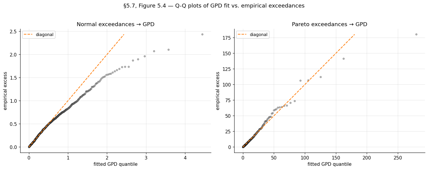
Example 6 (Standard Normal exceedances — Gumbel domain).
GPD MLE should recover (consistent with the Gumbel-domain prediction of in §3.4). The mean-excess plot should be approximately flat (slope at ) above the threshold. The notebook prints threshold , , GPD-MLE with wide SE (the Gumbel-domain is poorly identified at this because the tail is too thin to pin down precisely).
Example 7 (Pareto(α=2) exceedances — Fréchet domain).
GPD MLE should recover (consistent with §3.4’s ). Mean-excess plot should be linear with slope . The Hill plot should plateau at over a middle range of . The notebook prints threshold , , GPD-MLE (SE ), (SE ) — within of the truth .
VaR at and ES at the same level are computed for both examples. For the Pareto example, the analytical truth is and (using the closed-form for the standard Pareto with shape ); the GPD-fit-based estimate gives and , agreeing with the analytical truth to within for VaR and for ES.
6. Connections, ML applications, and limits
Sections 2–5 developed the asymptotic theory and inferential machinery of extreme value theory: max-stability and the trichotomy in §2, domains of attraction in §3, block-maxima inference in §4, and peaks-over-threshold inference in §5. This closing section steps back from the math. We discuss three modern ML applications that put the framework to work, sketch the natural follow-up topics that extend EVT in directions a typical practitioner will encounter, and lay out the cross-site map that locates this topic in the formalstatistics → formalML curriculum graph.
6.1 Three ML applications
Tail-aware prediction intervals. The prediction-intervals topic covers split conformal, conformalized quantile regression (CQR), and Hodges–Lehmann test-inversion intervals on a heteroscedastic regression problem with Student- residuals as one of its scenarios (the §4 heavy-tailed location-shift example there). Split conformal achieves nominal marginal coverage in that scenario, but pays for it with band widths nearly twice the homoscedastic-Gaussian case. Why? Because the tail is in — heavy enough that the residual distribution’s quantile is qualitatively larger than the Gaussian’s. The fitted GPD on residuals from §5 lets us decompose this bandwidth effect: on the residual distribution is exactly the half-width of an oracle-quantile prediction interval, and tells us how much further the typical conditional miscoverage extends past the band. For deployed regression models with heavy-tailed residuals — financial returns, queue latencies, certain biomedical responses — fitting a GPD to the residuals is a cheap and informative diagnostic that the standard CQR/conformal pipeline doesn’t surface.
A natural follow-up: replace the empirical quantile in CQR with a GPD-extrapolated quantile when the calibration set is small relative to the target . Conformal’s finite-sample guarantee holds for any score function, including a GPD-fitted one; the question is whether the GPD-fitted score has materially better conditional coverage in tail regimes. Initial work in this direction has shown promise (Chernozhukov–Wüthrich–Zhu 2018); a fuller treatment is beyond the scope of this section.
Out-of-distribution detection. A standard pattern in production ML is to monitor a scalar score per input — softmax confidence, energy, embedding norm, reconstruction error — and flag inputs where the score is unusually extreme as out-of-distribution. The classical baseline (Hendrycks–Gimpel 2017) uses a hard threshold on the maximum softmax probability; modern variants train an OOD-detection head or use likelihood ratios. The EVT contribution is principled threshold calibration: if we model the in-distribution score’s right tail as a GPD via §5’s machinery, then a candidate input’s “OOD-ness” becomes a calibrated tail probability — — rather than an uncalibrated raw score. This converts threshold tuning from a per-deployment hyperparameter into a single -level choice (“flag the top 0.1% of in-distribution scores as suspicious”), which generalizes across model versions and data drifts in a way raw thresholds do not.
The honest caveat: production OOD detection rarely fails at the right tail of a single score — it fails when the input violates assumptions the score doesn’t capture (covariate shift, novel object categories, adversarial inputs). EVT calibrates the tail; it does not detect the right tail of the right score. In production, this manifests as “EVT-calibrated OOD has well-controlled false-positive rates but mediocre true-positive rates on the failure modes that matter.” Treat the calibration as the floor, not the ceiling, of the OOD problem.
Tail-risk quantification for deployed models. A deployed model has a loss distribution — per-query latency, per-prediction error, per-decision regret — and the tails of that distribution are what determine real-world cost. The 99.9th percentile latency triggers SLA violations; the worst-case classification error over a deployment year is what regulators ask about. Estimating these from a finite history requires extrapolating past observed extremes, which is exactly what §4’s return-level machinery and §5’s POT-VaR-ES machinery are designed for. For a model deployed on queries per day with daily monitoring, a year of operation gives raw observations and daily-block-maxima — far more than enough for both block-maxima GEV and POT-GPD fits. The fitted models then give principled answers to “what loss is exceeded once a year on average” (a return level) or “what is the expected loss conditional on being in the worst 0.1% of queries” (an Expected Shortfall).
Two subtleties recur in production tail-risk work. First, daily blocks are usually not iid — diurnal cycles, day-of-week effects, and deployment changes induce serial dependence. The §6.2 forward-pointer to extremes-of-dependent-sequences is the relevant one. Second, the parent distribution drifts over time as the model and data change, so a single fitted GEV / GPD is not a stationary model — re-fitting on a rolling window is standard practice. The EVT framework is silent on both issues; they are handled by surrounding engineering.
6.2 Forward-pointers
Five directions extend the topic, each natural enough that a cross-reference is warranted, but with depth that pushes past this topic’s scope.
-
Extremes of dependent sequences. The Leadbetter–Lindgren–Rootzén (1983) framework introduces the extremal index that quantifies tail dependence: at the dependent sequence behaves like its iid counterpart for extreme-value purposes, while indicates clustering of extremes (one big event predicts another). The full theory generalizes the GEV trichotomy to weakly-dependent stationary sequences. For ML applications with serially-correlated losses, this is the right framework; the topic above silently assumes throughout.
-
Multivariate EVT and copula-based tail dependence. When the object of interest is the joint upper tail of a multivariate distribution rather than the univariate maximum, the GEV / GPD framework generalizes via the extreme-value copula and the spectral measure of tail dependence. The univariate marginals are still GEV / GPD; the dependence structure is encoded separately. Resnick (1987) and Beirlant–Goegebeur–Segers–Teugels (2004) are the standard references. ML applications include multivariate outlier detection and joint-quantile prediction.
-
Spatial extremes and max-stable processes. When the object of interest is the entire spatial field of extremes — extreme rainfall over a region, extreme network latencies across a service mesh — the framework generalizes further to max-stable processes. Davison, Padoan, and Ribatet (2012) is the standard practitioner introduction; Coles (2001), Chapter 9 has a textbook treatment. The mathematical machinery is more involved (the Pickands representation theorem for max-stable processes is the load-bearing result) and substantially beyond the scope of this topic.
-
Bayesian EVT. Frequentist GEV / GPD inference per §§4–5 has well-known difficulties at small or — wide confidence intervals, profile-likelihood asymmetries that delta-method intervals miss, and the boundary-MLE issues at . Bayesian methods sidestep many of these via informative priors on that exclude the pathological regime, plus full posterior inference over that captures asymmetry directly. Coles and Tawn (1996) and Stephenson (2016) give standard treatments; the Bayesian framework also opens the door to hierarchical EVT models that share information across blocks or thresholds. Variational Inference (coming soon) and Probabilistic Programming (coming soon) provide the inferential machinery.
-
Deep learning for EVT. Recent work has explored neural-network parameterizations of GEV / GPD parameters as functions of covariates — replacing the constant or with neural-network outputs that vary smoothly with input features. This is to EVT what mixture-density networks are to standard regression. The natural conformal-prediction connection — using a deep-learned GEV / GPD as a calibration model for tail-aware conformal scores — is, as far as we are aware, an open direction.
6.3 Limits
Three honest limitations of the framework as developed in this topic.
Asymptotic, not finite-sample. Both the GEV-of-block-maxima and GPD-of-exceedances results are asymptotic. At finite or finite , the parametric families are approximations whose error depends on how fast the parent’s tail enters the regular-variation regime. Second-order regular variation theory (de Haan–Resnick 1996) provides quantitative bounds, but these involve constants that are difficult to estimate. In practice, residual diagnostics — Q-Q plots, mean-excess plots, parameter-stability plots — are the working assurance that the approximation is acceptable.
Tail-only. By construction, the framework cares only about the upper tail of the parent distribution. It says nothing about the bulk, and a fitted GEV / GPD is not a useful generative model for typical observations. For applications where both bulk and tail matter — full-distribution density estimation, simulation, generative modeling — EVT provides one component (the tail) of a hybrid model whose body is fit by other means (kernel density estimation, parametric models, deep generative models). The hybrid construction is itself non-trivial; Carreau and Bengio (2009) discuss the body-tail-stitching problem.
Univariate. The topic treats only univariate extremes. Multivariate generalizations exist (the §6.2 forward-pointer), but the formalism becomes substantially more involved. For ML applications where the natural object is a multivariate loss vector or a high-dimensional embedding, the univariate framework applies to scalar summaries (norms, projections) but loses the joint tail-dependence structure.
A meta-point worth making: the asymptotic theory’s universality is its great virtue and its great limit. Trichotomy says we don’t need to know the parent — the limit is one of three families. But the limit is only one of three families, and choosing among them at finite samples is the inferential burden of §§4–5. Get wrong, and the extrapolation goes badly wrong, in directions the parametric family doesn’t constrain.
Connections and Further Reading
Extreme value theory sits at a specific location in the formalstatistics → formalML curriculum graph. The backward pointers (prerequisites) and forward pointers (where this topic shows up downstream) are worth surfacing explicitly.
Backward to formalstatistics.
-
formalStatistics: Empirical Processes . The Donsker / functional-CLT machinery is the framework for “what happens to the entire empirical CDF as .” EVT is the analog at the tail. The technical machinery overlaps in the slow-variation arguments of §3 and the regular-variation expansions of §5. Referenced primarily in §3.
-
formalStatistics: Order Statistics & Quantiles . The sample maximum is the extreme order statistic; that topic treats the joint distribution of and the asymptotic theory of for fixed . EVT continues this story for (the maximum) and close to 1 (high quantiles via §5 POT). Referenced primarily in §1, §4, and §5.
Backward to formalcalculus.
- formalCalculus: Sigma-Algebras & Measures . The weak-convergence framework that all of §§2–3 lean on lives there — convergence-in-distribution as weak convergence of probability measures, the Portmanteau theorem (used in the Khintchine proof of §2.3), and Slutsky’s theorem (used implicitly throughout). Referenced in §§2–3.
Internal to formalML.
- Concentration Inequalities. The sub-Gaussian / sub-exponential machinery there is the lead-in to “what happens when those moment-bound assumptions fail” — and the Fréchet domain of §3 is exactly the answer.
- Prediction Intervals. T4 sibling. The heavy-tailed-residual scenario in
prediction-intervals§4 uses Student- residuals, which are in ; this topic’s §6.1 discusses GPD-extrapolated quantiles as a refinement of CQR for that regime.
Connections
- Topic predecessor on the Probability & Statistics track. The sub-Gaussian / sub-exponential machinery of concentration-inequalities §§4–5 is the lead-in to the Fréchet-domain treatment of §3 — what happens when the moment-bound assumptions of concentration fail. The §1.1 CLT-companion framing of EVT also uses concentration's framing of tail-bound regimes. concentration-inequalities
- T4 sibling. The heavy-tailed-residual scenario in prediction-intervals §4 uses Student-$t_3$ residuals, which fall in $\mathrm{DA}(\mathrm{Fr\acute{e}chet}_3)$; §6.1 of this topic discusses GPD-extrapolated quantiles as a refinement of conformal-quantile regression for that regime. prediction-intervals
- T4 track closer. Depth and EVT are duals: EVT studies the outermost observations (block maxima, threshold exceedances), depth studies the innermost (the median, deep regions). They combine in multivariate EVT where shallow-depth observations identify candidate extremes and depth contours bound the central mass against which extremes are measured. statistical-depth
References & Further Reading
- paper Limiting Forms of the Frequency Distribution of the Largest or Smallest Member of a Sample — Fisher & Tippett (1928) The original statement of the trichotomy used in Theorem 2 (Mathematical Proceedings of the Cambridge Philosophical Society).
- paper Sur la distribution limite du terme maximum d'une série aléatoire — Gnedenko (1943) The complete proof of the trichotomy and the domain-of-attraction characterizations of Theorems 3–5 (Annals of Mathematics).
- paper Statistical Inference Using Extreme Order Statistics — Pickands (1975) The unbounded-support half of the Pickands–Balkema–de Haan theorem (Theorem 7 here) plus the Pickands tail-index estimator of §5.5 (Annals of Statistics).
- paper Residual Life Time at Great Age — Balkema & de Haan (1974) The bounded-support companion to Pickands 1975, jointly forming Theorem 7 (Annals of Probability).
- paper A Simple General Approach to Inference About the Tail of a Distribution — Hill (1975) The Hill estimator of §5.5 and its consistency analysis under regular variation (Annals of Statistics).
- paper Estimation of the Generalized Extreme-Value Distribution by the Method of Probability-Weighted Moments — Hosking, Wallis & Wood (1985) The PWM estimator of §4.3, with the small-sample superiority over MLE documented in a Monte Carlo study (Technometrics).
- paper Maximum Likelihood Estimation in a Class of Nonregular Cases — Smith (1985) Theorem 6 here: GEV MLE asymptotic normality plus the $\xi > -1/2$ / $\xi \in (-1, -1/2]$ / $\xi \le -1$ regime distinction (Biometrika).
- paper Estimating Tails of Probability Distributions — Smith (1987) Theorem 8 here: GPD MLE asymptotics and the closed-form covariance matrix used for delta-method standard errors in §5.6 (Annals of Statistics).
- paper A Moment Estimator for the Index of an Extreme-Value Distribution — Dekkers, Einmahl & de Haan (1989) The DEdH moment estimator of §5.5; consistent across the full $\xi$ parameter range, in contrast to Hill's $\xi > 0$ restriction (Annals of Statistics).
- paper Laws of Large Numbers for Sums of Extreme Values — Mason (1982) Theorem 9 here: Hill estimator consistency and asymptotic normality under intermediate-sequence conditions (Annals of Probability).
- book Modeling Extremal Events for Insurance and Finance — Embrechts, Klüppelberg & Mikosch (1997) Principal reference for §§2–5. Chapter 3 covers the trichotomy, regular variation, and the Pickands–Balkema–de Haan theorem (Springer).
- book An Introduction to Statistical Modeling of Extreme Values — Coles (2001) Practitioner-oriented complement to EKM. Chapter 3.3.3 covers profile-likelihood intervals for return levels (§4.4 here); Chapter 4 covers POT inference (Springer).
- book Extreme Values, Regular Variation, and Point Processes — Resnick (1987) The advanced-theory reference for the Gumbel domain (Theorem 5 here, von Mises sufficient condition) and the de Haan class $\Pi$ (Springer).
- book Regular Variation — Bingham, Goldie & Teugels (1987) Standard reference for slow variation and Karamata's theorems used in §3 (Cambridge University Press).
- paper Coherent Measures of Risk — Artzner, Delbaen, Eber & Heath (1999) The coherent-risk-measure axioms that distinguish Expected Shortfall (subadditive) from Value-at-Risk (not subadditive); §5.6 references this (Mathematical Finance).
- paper A Baseline for Detecting Misclassified and Out-of-Distribution Examples in Neural Networks — Hendrycks & Gimpel (2017) The maximum-softmax-probability OOD baseline that §6.1 reformulates via GPD calibration (ICLR).