Bayesian Neural Networks

Overview

A trained neural network gives us a function, but it does not tell us how confident to be in that function. A point-estimate classifier confidently extrapolates its decision rule into regions where no training data lives, with no language for “I don’t know.” Bayesian neural networks are the response: instead of a single weight vector $w^*$ that minimizes a training loss, we work with a distribution $p(w \mid \mathcal{D})$ over weights and integrate predictions against it, so predictive variance grows where the data has nothing to say. The catch is that $p(w \mid \mathcal{D})$ is a distribution on $\mathbb{R}^p$ for $p$ on the order of $10^4$ to $10^9$, and the posterior is intractable in four distinct ways for any non-trivial network.

This topic develops the practical recipes that make BNN inference work at deep-learning scale. §1 frames the problem on a 2D Two Moons toy classifier so the picture is visible. §2 lifts the geometric picture into a formal weight-space posterior, derives the weight-decay-as-MAP identity, and explains the three structural ways the Bernstein–von Mises asymptotic fails for neural networks. §§3–7 develop five recipes for fitting the posterior — Laplace approximation, MC-dropout, deep ensembles, stochastic-gradient Langevin dynamics (SGLD), and stochastic-gradient HMC (SGHMC) — each addressing a different subset of the §2.4 obstacles. §8 evaluates them head-to-head on calibration metrics: expected calibration error, the Brier score, and negative log-likelihood as a proper scoring rule, plus the epistemic-aleatoric decomposition and the cold-posterior effect. §9 closes with the function-space view from the neural network Gaussian process (NNGP, Neal 1996) and the neural tangent kernel (NTK, Jacot et al. 2018), which ties weight-space methods to the Gaussian Processes machinery.

This is the sixth topic of T5 Bayesian & Probabilistic ML, after Variational Inference, Gaussian Processes, Probabilistic Programming, Mixed-Effects Models, and Stacking & Predictive Ensembles. It is the T5 flagship — the topic where the substrate of the prior five topics (variational families, GP machinery, model declaration, hierarchical structure, predictive averaging) gets combined into the catalog of methods practitioners actually reach for when the model is a deep network and uncertainty matters.

1. Why Bayesian over the weights

A trained neural network gives us a function, but it does not tell us how confident to be in that function. A point-estimate classifier on the Two Moons distribution — two interleaving crescents in $\mathbb{R}^2$, separable by a smooth nonlinear boundary, contaminated with isotropic noise — produces a single decision rule and confidently extrapolates that rule into regions where no training data lives. The rule is wrong somewhere, but the model has no way to say where. For an ML practitioner, this is a structural problem: medical-imaging classifiers, autonomous-vehicle perception models, and clinical-decision-support systems all need to know when they don’t know. A model that returns “99% confident” everywhere — including on inputs unlike anything it has ever seen — is a liability.

Bayesian neural networks are the response. Instead of a single weight vector $w^* \in \mathbb{R}^p$ that minimizes a training loss, we work with a distribution $p(w \mid \mathcal{D})$ over weights, conditioned on the training data $\mathcal{D} = \{(x_i, y_i)\}_{i=1}^n$. Predictions integrate over that distribution. This topic is the catalogue of practical recipes for building, fitting, and reading that distribution when the model has thousands or millions of weights and the posterior is intractable in every standard sense. §§3–7 develop five recipes — Laplace approximation, MC-dropout, deep ensembles, SGLD, SGHMC. §8 evaluates them head-to-head on calibration. §9 closes with the function-space view. This section frames why the recipes are needed and what they share.

1.1 What a point-estimate model can’t tell us

Fix notation. A neural network with weights $w \in \mathbb{R}^p$ is a parametric function $f_w : \mathcal{X} \to \mathcal{Y}$ assembled from compositions of affine maps and elementwise nonlinearities. For binary classification, $\mathcal{Y} = \{0, 1\}$ and the model produces a real-valued logit $f_w(x) \in \mathbb{R}$ which we squash through the logistic sigmoid $\sigma(z) = (1 + e^{-z})^{-1}$ to get a class-1 probability $\sigma(f_w(x))$. The likelihood under the Bernoulli observation model is $p(y \mid x, w) \;=\; \sigma(f_w(x))^y \bigl(1 - \sigma(f_w(x))\bigr)^{1 - y}.$

A point-estimate network minimizes a regularized cross-entropy loss $w^* \;=\; \arg\min_{w \in \mathbb{R}^p}\,\Bigl\{ -\sum_{i=1}^n \log p(y_i \mid x_i, w) + \tfrac{\lambda}{2}\|w\|^2 \Bigr\}$ using stochastic gradient descent or one of its momentum variants, and returns the single learned weight vector $w^*$. At test time the model produces a single predicted probability $\sigma(f_{w^*}(x^*))$. Two things are missing.

The first is uncertainty about the prediction. The model returns a number near $0$ or near $1$, with no companion estimate of how much that number would change under a different reasonable choice of $w$. The second is uncertainty about $w$ itself. The training loss is non-convex in $w$; the SGD trajectory ends in some local minimum determined by initialization, batch order, and learning-rate schedule; a different run with a different seed lands in a different minimum, with potentially different predictions far from the training data. The point estimate $w^*$ is one of many plausible weight vectors, and the model has no language for that fact.

1.2 The predictive distribution and the four obstacles

The Bayesian fix is to replace $w^*$ with the full posterior. Place a prior $p(w)$ on the weights — typically the isotropic Gaussian $\mathcal{N}(0, \tau^2 I_p)$ that pairs with the $\ell_2$ regularizer above (§2.2 makes this correspondence explicit). Bayes’ rule gives $p(w \mid \mathcal{D}) \;=\; \frac{p(\mathcal{D} \mid w)\,p(w)}{p(\mathcal{D})}, \qquad p(\mathcal{D}) \;=\; \int p(\mathcal{D} \mid w)\,p(w)\,dw,$ where $p(\mathcal{D} \mid w) = \prod_{i=1}^n p(y_i \mid x_i, w)$ is the likelihood of the training data under weights $w$. The predictive distribution at a new input $x^*$ marginalizes the weights out: $p(y^* \mid x^*, \mathcal{D}) \;=\; \int p(y^* \mid x^*, w)\,p(w \mid \mathcal{D})\,dw.$

Where the data is dense, plausible weight settings agree on what $y^*$ should be, and the integral concentrates — predictive variance is small. Where the data is sparse, plausible weight settings disagree, the integral spreads, and predictive variance grows. The model knows when it doesn’t know, because “I don’t know” is encoded as breadth in the weight posterior.

The catch is that $p(w \mid \mathcal{D})$ is a distribution on $\mathbb{R}^p$ for $p$ on the order of $10^4$ to $10^9$, and the posterior is intractable in four distinct ways. The marginal likelihood $p(\mathcal{D})$ has no closed form for any non-trivial network, so we cannot evaluate $p(w \mid \mathcal{D})$ pointwise without an approximation. The negative log-likelihood is deeply non-convex in $w$: by symmetry, every loss-landscape mode has copies under permutations of the hidden units, and the modes are separated by sharp ridges where Gaussian approximations break down. The dimension $p$ is high enough that vanilla MCMC mixes too slowly to be useful at deep-learning scale. And the likelihood gradient $\nabla_w \log p(\mathcal{D} \mid w) = \sum_{i=1}^n \nabla_w \log p(y_i \mid x_i, w)$ requires a full pass over $\mathcal{D}$ — feasible for $n$ in the hundreds, infeasible for the millions that motivate using a neural network in the first place.

Every method in this topic is an answer to one of these obstacles. Laplace approximation (§3) gives up on the multimodal structure and fits a single local Gaussian centered at the MAP estimate — cheap and asymptotically justified by the Bernstein–von Mises theorem from formalStatistics: Central Limit Theorem that §2 imports from formalstatistics. MC-dropout (§4) reinterprets the dropout regularizer used at training time as a Bernoulli variational posterior and turns the deterministic predictor’s stochastic forward passes into Monte Carlo posterior samples — almost free, but the variational family is rigid. Deep ensembles (§5) abandon weight-space inference altogether and treat $K$ independently-trained networks as approximate samples in function space — empirically the strongest of the cheap methods, but the theoretical justification is delicate. Stochastic-gradient Langevin dynamics (§6) and stochastic-gradient HMC (§7) bring the asymptotic exactness of MCMC into the deep-learning regime by injecting calibrated Gaussian noise into mini-batch gradient updates — the noise compensates for the bias mini-batching introduces, and the resulting stochastic process has the posterior as its stationary distribution.

1.3 The geometric picture and the road ahead

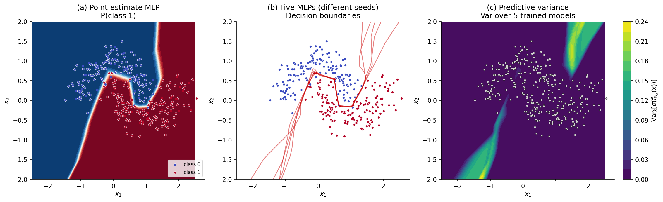
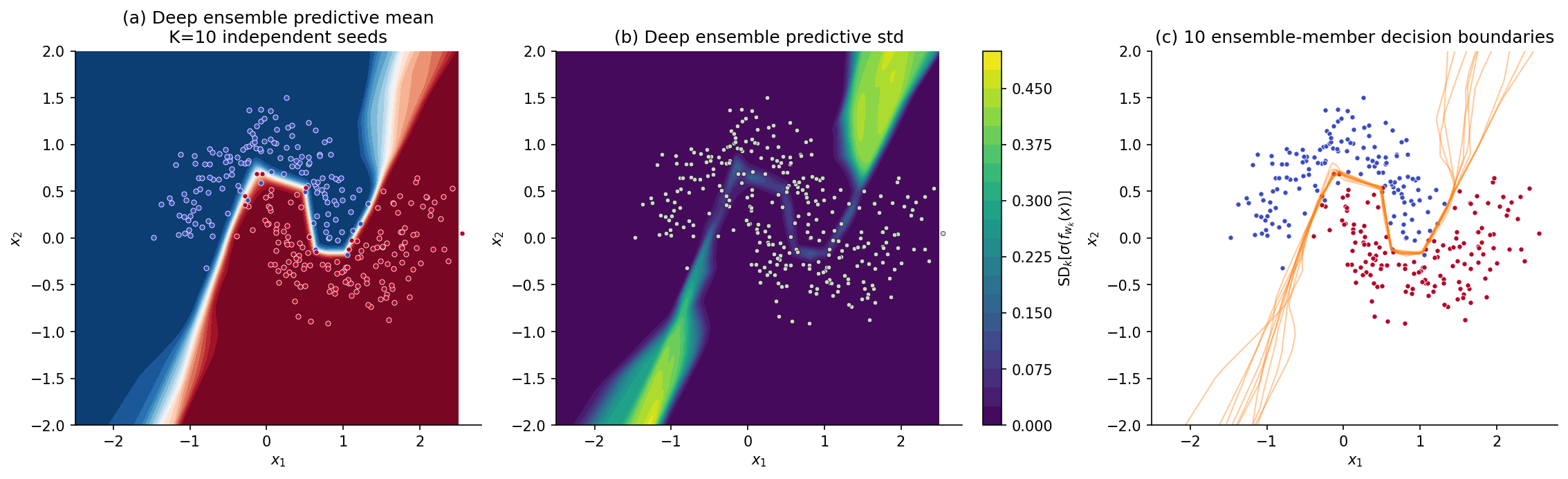
For the rest of this section we work on a 2D toy classifier so the picture is visible. Data are drawn from Two Moons with noise level $0.20$ at $n = 300$ points. We fit a small MLP — three hidden layers, 32 ReLU units each — by minimizing the regularized binary cross-entropy loss with $\lambda = 10^{-4}$ for 200 Adam epochs. The point-estimate model gives the decision surface in panel (a) of Figure 1: a clean boundary separating the two classes, with predicted probabilities near $0$ or near $1$ across most of the input space — high confidence even at distances from the data where any honest model should hesitate.

To see what an honest predictive distribution looks like we fit five copies of the same architecture from independent random initializations. Panel (b) overlays the five $0.5$-probability decision boundaries. Where the data is dense, the boundaries agree and the overlay is sharp. Far from the data — in the corners of the input frame — the boundaries fan out: five plausible models trained on the same data give five different answers in the regions where the data has nothing to say. Panel (c) renders the disagreement as a heatmap of predictive variance over the input space, the variance of the predicted class-1 probabilities across the five models. Bright regions are where the model knows it doesn’t know. The five-model ensemble previewed here is the embryo of every method in this topic, and §5 formalizes it as a deep ensemble; §§3, 4, 6, 7 will produce comparable heatmaps from very different mechanisms.

A second axis of uncertainty matters too. If two data points sit in the same input neighborhood but carry different class labels — which Two Moons can produce in the strip between the crescents at high noise — no model on any architecture can confidently predict that neighborhood. That is aleatoric uncertainty: irreducible noise inherent in the data-generating process. The variance from disagreement among trained models is epistemic uncertainty: it reflects what the model would learn from more data, not what no model can ever learn. §8 disentangles the two formally; for now we note that BNNs primarily address epistemic uncertainty, and that a calibrated BNN should report large epistemic variance off-distribution and large aleatoric variance in noisy regions of the support.

The §2 derivation lifts this geometric picture into a formal weight-space posterior — the object the rest of the topic approximates. With that machinery in hand, §3 fits its first Bayesian neural network.

Loading…

2. The weight-space posterior

The §1 picture — a model that should report breadth of plausible weight settings as predictive variance — is geometric. §2 lifts it into formal mathematics. The deliverable of this section is four facts: (i) the posterior under a Gaussian weight prior has a closed-form negative-log expression; (ii) maximizing that posterior is equivalent to L2-penalized empirical-risk minimization, so the well-known weight decay regularizer is a maximum-a-posteriori estimator under a specific prior; (iii) the Bayesian central-limit theorem (Bernstein–von Mises) guarantees that, in well-specified parametric models, the posterior asymptotically concentrates as a Gaussian centered at the MLE; and (iv) the regularity conditions for that theorem fail for typical neural networks, in three specific ways that motivate the four approximation strategies of §§3–7.

2.1 The Gaussian-prior MLP

Fix a parametric MLP $f_w: \mathcal{X} \to \mathbb{R}$ with weights $w \in \mathbb{R}^p$. For binary classification the conditional distribution of the label given the input is Bernoulli with logit $f_w(x)$: $p(y \mid x, w) \;=\; \sigma(f_w(x))^y \bigl(1 - \sigma(f_w(x))\bigr)^{1 - y},$ where $\sigma(z) = (1 + e^{-z})^{-1}$ is the logistic sigmoid. We complete the model with a Gaussian prior on the weights:

The choice of $\tau^2 I_p$ as the prior covariance is the default in the BNN literature and the one we’ll work with throughout. It assumes weights are a priori independent and identically distributed — a strong assumption that ignores all structure in the weight tensor (layer, channel, position) but keeps the math tractable. Heavy-tailed and hierarchical priors are the subject of Sparse Bayesian Priors; per-layer prior scales are revisited in §8.5’s cold-posterior remark. For now, $\tau$ is a single scalar hyperparameter — large $\tau$ is a weak prior (close to MLE), small $\tau$ is a strong prior (heavy regularization).

2.2 The negative log-posterior, and weight decay as a Bayesian prior

Take the negative log of the posterior: $-\log p(w \mid \mathcal{D}) \;=\; -\log p(\mathcal{D} \mid w) \;-\; \log p(w) \;+\; \log p(\mathcal{D}).$ The first term is the negative log-likelihood — the cross-entropy training loss (modulo signs). The second is a quadratic in $w$, since the prior is Gaussian: $-\log p(w) = \frac{1}{2\tau^2}\|w\|_2^2 + \mathrm{const}_{\tau, p}$, where the constant absorbs $\log\bigl((2\pi\tau^2)^{p/2}\bigr)$. The third does not depend on $w$. Stripping $w$-independent constants we get $-\log p(w \mid \mathcal{D}) \;=\; -\sum_{i=1}^n \log p(y_i \mid x_i, w) \;+\; \frac{1}{2\tau^2}\|w\|_2^2 \;+\; C,$ where $C$ is a constant in $w$. This is structurally the L2-penalized cross-entropy training loss with regularization strength $\lambda = 1/\tau^2$.

Three corollaries are worth pulling out, each with downstream consequences for §§3–8.

Weight decay is a Bayesian regularizer. The standard “weight decay” hyperparameter $\lambda$ in deep-learning libraries has a Bayesian interpretation: $\lambda$ is the inverse variance of the implicit Gaussian prior on the weights, $\lambda = 1/\tau^2$. A weight-decay-trained model with $\lambda = 10^{-4}$ is the MAP estimator under a $\mathcal{N}(0, 10^4\, I_p)$ prior on each weight. The choice of $\lambda$ is therefore a choice of prior, and “tuning $\lambda$ on a validation set” is empirical-Bayes hyperparameter selection. This is the canonical home for the cross-cutting concept of weight decay — the slug never gets its own page; the concept lives here.

The MAP is the starting point for §3. The Laplace approximation builds a Gaussian posterior approximation centered at $\hat{w}_{\mathrm{MAP}}$. Because $\hat{w}_{\mathrm{MAP}} = \hat{w}_{\mathrm{WD}}$, any standard PyTorch model trained with weight decay is already the center of a Laplace approximation; we just haven’t computed the surrounding curvature yet. §3 fills in that missing piece.

The cold-posterior caveat. Many BNN practitioners empirically find that tempered posteriors $p(w \mid \mathcal{D})^{1/T}$ with $T < 1$ — equivalently, larger $\lambda$ than the prior naturally specifies — give better-calibrated predictions than the strict Bayesian $T = 1$. This is the “cold-posterior effect” (Wenzel et al. 2020) and indicates that the Gaussian prior is misspecified for typical training datasets: the data effectively want a stronger regularizer than the principled $\lambda = 1/\tau^2$ delivers. The phenomenon is one of the central open problems in BNNs and is treated formally in §8.5.

2.3 The Bernstein–von Mises asymptotic

What does the weight-space posterior look like for large $n$? The classical result is the Bayesian central-limit theorem, also known as Bernstein–von Mises:

The proof is the subject of formalstatistics’s central-limit-theorem topic. In words: the posterior, recentered at the MLE and rescaled by $\sqrt{n}$, converges in total variation to a Normal distribution with covariance equal to the inverse Fisher information. Equivalently, for large $n$ the un-rescaled posterior is approximately $p(w \mid \mathcal{D}_n) \;\approx\; \mathcal{N}\!\Bigl(w^*_n,\; \tfrac{1}{n}\, I(w_0)^{-1}\Bigr),$ a Gaussian centered at the MLE with covariance the inverse total Fisher information $H_n^{-1} \approx (n I(w_0))^{-1}$.

This is the asymptotic license for §3’s Laplace approximation. Under BvM, fitting a Gaussian centered at the MAP with the right curvature gives a posterior approximation that is exact in the $n \to \infty$ limit. The Laplace construction in §3 will use the observed Fisher information $H_n = -\nabla^2 \log p(w \mid \mathcal{D}_n) \big|_{w = \hat{w}_{\mathrm{MAP}}}$, which differs from $n I(w_0)$ by a fluctuation that is itself $O(\sqrt{n})$. The point is: there is a principled reason to expect the posterior to be approximately Gaussian centered at the MAP for large $n$, provided the regularity conditions hold.

2.4 Why Bernstein–von Mises fails for neural networks

The regularity conditions for BvM are: $p$ fixed, model well-specified, MLE consistent and asymptotically Normal, Fisher information matrix positive-definite at $w_0$, posterior absolutely continuous with respect to the prior. These conditions fail for typical neural networks in three structural ways.

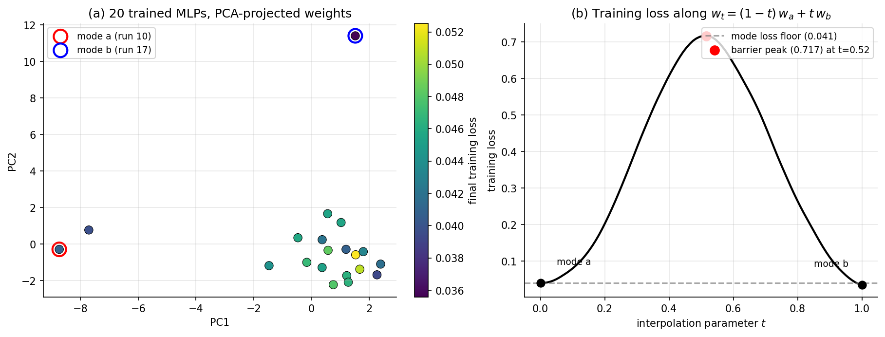
Hidden-unit permutation symmetry. Consider an MLP layer with $h$ hidden units, $W \in \mathbb{R}^{d \times h}$ input weights and $b \in \mathbb{R}^h$ biases. Permuting the columns of $W$ (and the corresponding entries of $b$ and the next layer’s row weights) gives an exactly equivalent function. So the function $f_w$ is invariant under $S_h$, the symmetric group on $h$ elements. The likelihood $p(\mathcal{D} \mid w)$ inherits this symmetry, and so does the posterior. There are at least $h!$ identical modes per hidden layer. For a 32-unit layer, $32! \approx 10^{35}$. The posterior has more than $10^{35}$ identical modes, separated by ridges of low likelihood — interpolating linearly between two modes via $w_t = (1 - t) w_a + t w_b$ does not generally produce another mode, since the loss along the interpolation rises through a barrier. Vanilla MCMC can mix over the connected component of the posterior support that it starts in, but cannot in finite wall-clock time mix between disconnected modes. BvM’s “single Gaussian centered at the MLE” is wrong globally because there is no single MLE.

ReLU positive scaling. For ReLU activations, $\mathrm{ReLU}(c\, z) = c \cdot \mathrm{ReLU}(z)$ for any $c > 0$. So if we multiply the input weights to a hidden unit by $c > 0$ and divide the outgoing weights by $c$, the function is unchanged: $f_w$ is invariant under the action of the multiplicative group $(\mathbb{R}_{>0})^h$ on weights. This is a continuous symmetry, not a discrete one, and it means that even within a single permutation class the MLE is not isolated — it sits on a $h$-dimensional submanifold of equally-good weights. The Fisher information matrix is singular along this submanifold (the gradient of the log-likelihood is zero in those directions because the function does not change), so BvM’s invocation of $I(w_0)^{-1}$ as a positive-definite covariance fails. Weight decay breaks the symmetry by penalizing rescalings — $\|c\, w_{\mathrm{in}}\|^2 + \|w_{\mathrm{out}} / c\|^2$ is minimized at a specific $c$ — so the MAP is locally unique even when the MLE is not. But the underlying likelihood is not strongly identified.

Over-parametrization. Modern deep networks have $p \gg n$. ResNet-50 has $\sim\!25 \times 10^6$ parameters; ImageNet has $\sim\!10^6$ training images. BvM operates in the regime $p$ fixed, $n \to \infty$. The opposite regime — $p \to \infty$ with $n$ fixed or growing slowly — is the regime of high-dimensional statistics, and the asymptotics there are different. The infinite-width limit of §9 makes one specific version of this regime tractable (function-space rather than weight-space), but for finite-width over-parametrized networks, BvM gives no asymptotic guidance.

These three failure modes organize the rest of the topic. Laplace (§3) gives up on the global picture and approximates the posterior locally at the MAP — accepting the failure of BvM globally and pursuing a local Gaussian that captures local curvature even if it misses the $h!$ permutation copies and the ReLU rescaling submanifold. MC-dropout (§4) uses a tractable but rigid variational family that sidesteps the exact-posterior question entirely. Deep ensembles (§5) sample $K$ approximate samples from $K$ different initializations, getting some coverage of distinct modes. SG-MCMC (§§6–7) accepts the multimodality and tries to mix between modes via Langevin dynamics on minibatches.

Training pool of 30 MLPs (~15 s)…

3. The Laplace approximation

§2 ends with a problem and a permission. The problem is that the true weight-space posterior $p(w \mid \mathcal{D})$ is intractable: no closed-form normalizer, more than $h!$ identical modes, and continuous symmetries that make the Fisher information singular within each mode. The permission is Bernstein–von Mises: under the regularity conditions the posterior is asymptotically a Gaussian centered at the MLE. The Laplace approximation accepts that the BvM regularity conditions don’t strictly hold globally but observes that they hold locally at any sufficiently regular minimum of the negative log-posterior — and builds a Gaussian approximation by Taylor-expanding around such a minimum. The construction goes back to Laplace’s 1774 calculation of the asymptotic value of $\int e^{-n h(\theta)}\,d\theta$; MacKay’s 1992 PhD thesis brought it into Bayesian neural networks; the modern revival is Daxberger et al. 2021 (laplace-torch), which scales the construction to ImageNet-class networks via Kronecker-factored curvature.

3.1 The construction

Let $U(w) := -\log p(w \mid \mathcal{D})$ be the negative log-posterior, modulo the unknown constant $\log p(\mathcal{D})$. From §2.2 we have $U(w) \;=\; -\sum_{i=1}^n \log p(y_i \mid x_i, w) \;+\; \frac{1}{2\tau^2}\|w\|_2^2 \;+\; \mathrm{const}.$ Suppose $\hat{w} := \hat{w}_{\mathrm{MAP}} = \arg\min_w U(w)$ is a local minimum at which $U$ is twice continuously differentiable and the Hessian $H := \nabla^2 U(w)|_{w = \hat{w}}$ is positive-definite. Taylor-expand $U$ to second order around $\hat{w}$: $U(w) \;=\; U(\hat{w}) \;+\; \nabla U(\hat{w})^\top (w - \hat{w}) \;+\; \tfrac{1}{2}(w - \hat{w})^\top H (w - \hat{w}) \;+\; O(\|w - \hat{w}\|^3).$ At a local minimum $\nabla U(\hat{w}) = 0$, so the linear term vanishes. Dropping the higher-order terms — the Laplace approximation itself — we get $U(w) \;\approx\; U(\hat{w}) \;+\; \tfrac{1}{2}(w - \hat{w})^\top H (w - \hat{w}).$ Exponentiating and renormalizing, $p(w \mid \mathcal{D}) \;\approx\; q(w) \;:=\; \mathcal{N}\bigl(w \,\big|\, \hat{w},\, H^{-1}\bigr).$ The construction takes a Gaussian whose mean is the MAP and whose precision is the local curvature of the negative log-posterior. Two further facts come for free.

The Hessian decomposes additively. From the form of $U$, $H \;=\; -\nabla^2_w \log p(\mathcal{D} \mid w)\big|_{w = \hat{w}} \;+\; \frac{1}{\tau^2} I_p \;=:\; H_{\mathrm{data}} + H_{\mathrm{prior}},$ the data Hessian plus the prior precision. The prior contribution is constant in $w$, isotropic, and explicitly positive-definite; it stabilizes the data Hessian when the latter has near-zero or negative eigenvalues from saddle directions or the §2.4 ReLU rescaling submanifold. In practice we either compute $H$ directly or compute $H_{\mathrm{data}}$ and add $\tau^{-2} I_p$ explicitly.

The marginal likelihood comes for free as a side effect. The Laplace approximation also gives a closed-form estimate of $p(\mathcal{D})$: $\log p(\mathcal{D}) \;\approx\; -U(\hat{w}) \;+\; \frac{p}{2}\log(2\pi) \;-\; \frac{1}{2}\log\det H,$ known as the Laplace marginal-likelihood approximation. This is the basis of Variational Bayes for Model Selection and the BIC’s asymptotic form (cross-link to formalstatistics’s formalStatistics: Model Selection and Information Criteria ).

3.2 Asymptotic exactness — and where it stops

The §2.4 caveats apply with full force here. The proof above assumes (i) $p$ fixed, (ii) $H_n$ positive-definite at $\hat{w}_n$, and (iii) the BvM regularity conditions. For neural networks: $p$ is not fixed in any meaningful sense (over-parametrization), $H_{\mathrm{data}}$ has near-zero eigenvalues from the ReLU rescaling submanifold (we rescue this with $H_{\mathrm{prior}} = \tau^{-2} I_p$, but the result is a Laplace approximation around an artificially regularized minimum), and the global posterior has many modes that the Laplace approximation around any one of them cannot represent. So Theorem 3.2 should be read as a local guarantee that the Gaussian fit is the best second-order approximation around $\hat{w}$, plus an asymptotic guarantee that this best approximation converges to the truth in well-specified parametric settings. For BNNs we get the local part and lose most of the asymptotic part.

This is enough for a useful method. The Laplace BNN’s predictive mean recovers the point estimate, its predictive variance grows away from the data exactly because the local quadratic in $U$ flattens away from $\hat{w}$, and the construction needs no sampling at all once $\hat{w}$ and $H$ are in hand. What it loses — multi-modality, ReLU-rescaling spread — is exactly what §§5–7 will recover.

3.3 The predictive distribution under linearization

A Gaussian posterior over weights does not directly give a Gaussian posterior over outputs, because $f_w(x)$ is a nonlinear function of $w$. The integral $p(y^* \mid x^*, \mathcal{D}) \;=\; \int p(y^* \mid x^*, w)\,q_{\mathrm{Lap}}(w)\,dw$ has no closed form. The standard reduction is first-order linearization of the network around the MAP: $f_w(x) \;\approx\; f_{\hat{w}}(x) \;+\; J(x)^\top (w - \hat{w}), \qquad J(x) := \nabla_w f_w(x)\big|_{w = \hat{w}}.$ Under this linearization, $f_w(x)$ is an affine function of $w$. If $w \sim \mathcal{N}(\hat{w}, H^{-1})$, then the logit $f_w(x)$ is Gaussian with mean $f_{\hat{w}}(x)$ and variance $J(x)^\top H^{-1} J(x)$.

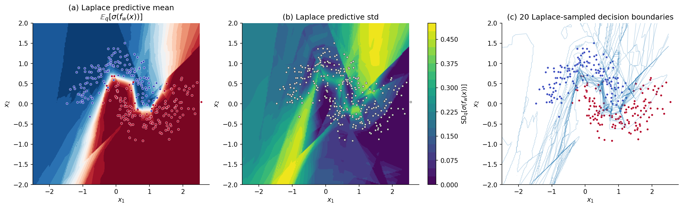
The factor $\pi/8$ comes from MacKay’s 1992 Gaussian-CDF approximation to the sigmoid: $\int \sigma(z) \mathcal{N}(z; m, v)\,dz \approx \sigma(m / \sqrt{1 + \pi v / 8})$. The reader sees the predictive variance $\tilde{v}(x)$ enter explicitly: where $\tilde{v}(x)$ is small (data-dense regions, where the network is well-determined), the predictive collapses to $\sigma(\tilde{m}(x))$ — the point estimate from §1. Where $\tilde{v}(x)$ is large (off-distribution regions, where small changes in $w$ produce large changes in $f_w(x)$), the predictive is squashed toward $0.5$ — the model’s confession of ignorance.

In practice we have two implementation choices for the predictive: (a) closed-form via Prop 3.3, computing $J(x)$ at each test point and the matrix product $J(x)^\top H^{-1} J(x)$; (b) Monte Carlo, sampling $w^{(s)} \sim \mathcal{N}(\hat{w}, H^{-1})$ and averaging $\sigma(f_{w^{(s)}}(x))$ over $s = 1, \ldots, S$ samples. For the §3.5 Two Moons figure we use (b) because it lets us also visualize sample decision boundaries; in production BNN libraries the closed-form (a) is faster.

3.4 Practical curvature

Computing and storing $H \in \mathbb{R}^{p \times p}$ for $p$ in the millions is impossible — $p^2$ memory, $O(p^3)$ inversion. Three standard reductions trade fidelity for tractability.

Last-layer Laplace (Daxberger et al. 2021). Fix all but the final linear layer’s weights at their MAP values; do Laplace only over the last layer. The last layer typically has $p_L \ll p$ parameters — for a 32-unit penultimate layer × $C$ output classes, $p_L \approx 32 C$. $H_{\mathrm{last\text{-}layer}} \in \mathbb{R}^{p_L \times p_L}$ is cheap. Empirically competitive with full Laplace on a wide range of tasks; the underlying intuition is that in over-parametrized networks, most of the weight-space uncertainty that affects predictions is concentrated in the final layer.

Kronecker-factored approximate curvature (KFAC; Martens & Grosse 2015). For each layer, approximate the Fisher information block as a Kronecker product $H_\ell \approx A_\ell \otimes G_\ell$, where $A_\ell$ is the input-activation second moment and $G_\ell$ is the output-gradient second moment. Storage cost reduces from $p_\ell^2$ to $\dim(A_\ell)^2 + \dim(G_\ell)^2$ per layer. The Kronecker assumption is structural (it ignores cross-layer covariance entirely), but matches the block-diagonal-plus-Kronecker structure of the Fisher information of natural-gradient methods.

Diagonal Fisher. Take only the diagonal of $H$. Cheapest possible — $O(p)$ memory — but discards all weight correlations. Often too aggressive: the diagonal Hessian eigenvalues are unreliable estimates of the full spectrum, and diagonal-Fisher Laplace BNNs frequently underestimate predictive variance in correlated directions.

For the §3.5 Two Moons example with $p = 2241$ parameters, full Laplace is feasible. For real-world BNNs, last-layer or KFAC is the practical choice; the laplace-torch library (Daxberger et al. 2021) implements all three reductions and is the default tool.

3.5 Algorithm and worked example

Algorithm 3.4 (Laplace-fit BNN).

Input: training data $\mathcal{D}$, network $f_w$, prior scale $\tau^2$, sample count $S$. Output: predictive distribution $\hat{p}(y \mid x)$ at test inputs.

1. Compute $\hat{w} := \arg\min_w U(w)$ via Adam or SGD with weight decay $\lambda = 1/\tau^2$.
2. Compute the data Hessian $H_{\mathrm{data}} := -\nabla^2 \log p(\mathcal{D} \mid w)|_{w = \hat{w}}$ via autodiff (or one of the §3.4 reductions).
3. Form $H := H_{\mathrm{data}} + \tau^{-2} I_p$ and stabilize: $H \leftarrow H + \delta I_p$ for small $\delta > 0$ if any eigenvalue is non-positive.
4. Cholesky-factor $H = L L^\top$.
5. Sample $z^{(s)} \sim \mathcal{N}(0, I_p)$ for $s = 1, \ldots, S$; set $w^{(s)} := \hat{w} + L^{-\top} z^{(s)}$.
6. Predict via $\hat{p}(y \mid x) := S^{-1} \sum_s p(y \mid x, w^{(s)})$, or via Prop 3.3’s closed-form.

The §1 first-seed model serves as $\hat{w}$. Step 2 uses torch.autograd.functional.hessian on the negative-log-posterior of the full training set; for $p = 2241$ this is $\sim\!2$ s on CPU. The $\tau^{-2} I_p$ contribution is automatic (we trained with weight decay $\lambda = 10^{-4}$, so $\tau^2 = 10^4$ and the prior precision contribution is $10^{-4} I_p$). Stabilization $\delta = 10^{-3}$ handles the residual ReLU-rescaling near-singularity. The Cholesky factorization on a $2241 \times 2241$ matrix is $\sim\!1$ s; sampling $S = 100$ posteriors and predicting on the $40{,}000$-point grid is $\sim\!3$ s.

Training MAP for Laplace approximation (~5 s)…

4. MC-dropout as approximate variational inference

The Laplace approximation of §3 builds a Gaussian posterior over weights from a single point estimate plus its local curvature. The construction is principled but expensive once the network is large — full Laplace needs $p^2$ Hessian storage, and even the §3.4 reductions (last-layer, KFAC) require non-trivial implementation effort. MC-dropout (Gal & Ghahramani 2016) is the cheap end of the BNN spectrum: it observes that a dropout-regularized network, trained the standard way, is already doing variational inference under a specific variational family, and that the only change needed at test time to extract a predictive distribution is to leave dropout on and average over $T$ stochastic forward passes. No new training, no Hessian, no extra hyperparameters beyond what dropout already requires. The trade is that the variational family is rigid in a way that systematically underestimates epistemic uncertainty in some regimes; §8’s calibration analysis quantifies the trade.

4.1 Recap: dropout as a regularizer

Dropout (Srivastava et al. 2014) trains a network by, at each minibatch, sampling a Bernoulli mask $b_\ell \in \{0, 1\}^{h_{\ell-1}}$ for each layer’s input activations with $b_{\ell, j} \sim \mathrm{Bernoulli}(\rho_\ell)$, multiplying activations elementwise by $b_\ell$ and rescaling by $1/\rho_\ell$ so the post-mask expected activation is unchanged. The forward pass uses the masked activations; the backward pass differentiates only through the unmasked units. At test time, dropout is conventionally turned off — the masks are replaced by the mean activation $\rho_\ell$ — and the resulting deterministic prediction is interpreted as an approximate average over the implicit ensemble of “thinned” subnetworks.

The standard story stops here: dropout is a regularizer, the deterministic test-time prediction is the answer, full stop. Gal & Ghahramani 2016 disrupt this by proving that the standard dropout training loss is, up to constants and a fixed prior choice, the negative ELBO of a specific variational posterior — and that to extract that posterior’s predictive distribution at test time, you don’t turn dropout off, you leave it on and Monte-Carlo over $T$ stochastic forward passes.

4.2 The Bernoulli variational family

Let the network have $L$ weight matrices $W_\ell \in \mathbb{R}^{h_{\ell-1} \times h_\ell}$, $\ell = 1, \ldots, L$. For each layer, define a Bernoulli mask matrix $Z_\ell$ as a diagonal matrix with $\mathrm{Bern}(\rho_\ell)$ entries on the diagonal: $Z_\ell = \mathrm{diag}(b_\ell), \qquad b_\ell \in \{0, 1\}^{h_{\ell-1}}, \qquad b_{\ell, j} \stackrel{\mathrm{iid}}{\sim} \mathrm{Bernoulli}(\rho_\ell).$ The variational weight matrix at layer $\ell$ is the random matrix $W_\ell^{\mathrm{var}} := M_\ell Z_\ell$, where $M_\ell \in \mathbb{R}^{h_{\ell-1} \times h_\ell}$ is a learnable mean weight matrix. Equivalently, the $j$-th column of $W_\ell^{\mathrm{var}}$ is either the $j$-th column of $M_\ell$ (with probability $\rho_\ell$) or the zero column (with probability $1 - \rho_\ell$).

This is a discrete variational family. At each evaluation, $W_\ell$ is one of $2^{h_{\ell-1}}$ possible matrices, parametrized by which subset of $M_\ell$‘s columns are zeroed. The family is rigid: $\rho_\ell$ is a fixed hyperparameter, not learned (Concrete dropout in §4.5 lifts this), and the structure of the variational posterior is determined entirely by the network’s architecture and the choice of which activations to drop.

4.3 The Gal–Ghahramani equivalence

The theorem’s content is that the same algorithm — minibatch SGD on cross-entropy plus $L_2$, with Bernoulli masks at each forward pass — can be read in two ways. The frequentist reads it as “regularized empirical-risk minimization with dropout noise”; the Bayesian reads it as “variational inference under the Bernoulli family.” Both readings yield the same trained network. The Bayesian reading does, however, instruct us to do something different at test time.

4.4 The MC-dropout predictive

The standard test-time recipe — turn dropout off and use the deterministic mean network — corresponds, in the variational reading, to evaluating $f_{\boldsymbol{M}}(x)$ at the mean weights, which is the MAP-style point estimate under $q_{\boldsymbol{M}}$. To get a Bayesian predictive distribution we leave dropout on and Monte-Carlo:

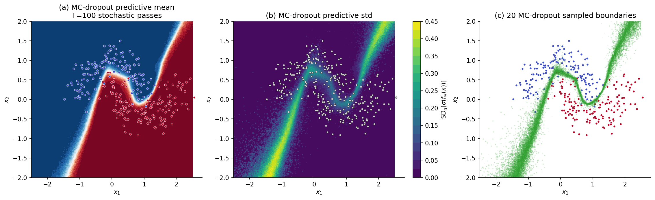
In code, this is two lines: keep the model in train() mode (which leaves dropout active) at test time and run $T$ forward passes. The single hyperparameter is $T$. Practical choice: $T \in [10, 100]$ for visual-quality predictive heatmaps, $T \geq 50$ for stable calibration-metric estimates (§8).

4.5 Limits and extensions

The Bernoulli family is rigid in a specific way: each weight column is either kept exactly (with probability $\rho$) or zeroed exactly (with probability $1 - \rho$). The family cannot represent continuous deviations from the mean weights — it has zero probability mass on weight matrices that are slightly perturbed from $M_\ell$ but not exactly some Bernoulli-masked version. Compared to the §3 Laplace family (a full Gaussian with covariance $H^{-1}$), MC-dropout has dramatically less expressive power. This shows up in three places.

Loading…

5. Deep ensembles as a function-space posterior proxy

The §3 Laplace approximation and §4 MC-dropout share a structural limitation: each parametrizes a single mode of the loss landscape. Laplace’s Gaussian is centered at one MAP; MC-dropout’s Bernoulli posterior puts its mass around one mean weight matrix $\boldsymbol{M}$. Neither captures the §2.4 hidden-unit permutation symmetry, the §2.4 ReLU rescaling submanifold, or any of the genuinely separated modes that §2’s Figure 2 made visible. Deep ensembles (Lakshminarayanan, Pritzel & Blundell 2017) take the opposite tack: don’t fit a parametric posterior at all. Instead, train $K$ networks from independent random initializations, treat the $K$ trained weight vectors as approximate samples from $K$ different modes of the posterior, and report the ensemble’s predictive as an equal-weighted mixture. The construction is brutally simple — the entire method is “train more times” — but it consistently outperforms more sophisticated single-mode methods on calibration and out-of-distribution detection benchmarks. Wilson & Izmailov 2020 articulate the why: deep ensembles are a coarse but legitimate function-space approximation to the Bayesian posterior predictive, in a regime where the function-space view dominates the weight-space view.

5.1 The construction

Two technical points are worth pulling out before the theory.

First, random initialization is essential — without it, the $K$ networks are identical. The standard recipe in PyTorch is to draw $\hat{w}^{(k)}_{0} \sim$ Kaiming-normal (or Xavier-normal, for older networks), with the random seed varied across $k$. The data and the optimizer are otherwise identical: same minibatches, same learning rate, same weight decay, same number of epochs.

Second, the ensemble is heterogeneous in function space even when each member is well-trained. Two networks trained from different initializations on the same data converge to different points in weight space (§2.4’s argument that there is no unique MLE), and although they typically agree on the training data, they extrapolate differently — exactly the §1 observation that motivated the topic.

The construction has no hyperparameters beyond $K$. No Hessians, no variational parameters, no Bernoulli rates, no learning-rate schedules for sampling. It is the simplest possible BNN method and, as §8 will show, often the most accurate.

5.2 The function-space-posterior interpretation

Why does training $K$ models with different initializations approximate the Bayesian posterior predictive? The argument has two layers.

The theorem’s preconditions are gross idealizations: real posteriors are not collapsed Diracs, real ensembles do not perfectly cover all $K$ modes, and the assumption of equal posterior mass across modes is a strong identifiability condition. But the spirit of the result is the right intuition. A deep ensemble is the right approximation to the Bayesian predictive in a function-space regime where (i) the posterior has multiple modes, (ii) the within-mode predictive variance is small relative to the between-mode predictive variance, and (iii) the modes have comparable posterior mass. For BNNs trained with weight decay, conditions (i) and (iii) hold approximately by §2.4’s symmetry arguments — every mode has $h!$ permutation copies, each with the same posterior mass — and (ii) holds whenever the network has sufficient capacity to fit the training data (the within-mode predictive variance shrinks as the network overfits).

The function-space view of Wilson & Izmailov 2020 makes this explicit. The Bayesian posterior over functions is $p(f \mid \mathcal{D}) \;=\; \int p(f \mid w)\,p(w \mid \mathcal{D})\,dw,$ where $p(f \mid w) = \delta(f - f_w)$ is the deterministic mapping from weights to functions. Distinct weight modes that produce the same function on the training data are redundant in function space — they all map to the same point $f$. Distinct weight modes that produce different functions on the training data correspond to different points in function space, and a deep ensemble’s diversity in function space is what matters for predictive uncertainty.

5.3 The mixture predictive form

For regression with Gaussian observation noise, each ensemble member’s predictive is Gaussian, and the ensemble predictive is a mixture of Gaussians with closed-form moments. This is the cleanest setting in which to read the epistemic-vs-aleatoric decomposition that §8 formalizes.

The decomposition is structural: aleatoric uncertainty is the noise level the model assumes (irreducible by adding more data), and epistemic uncertainty is the variance across ensemble members (reducible by adding more data, which would shrink each mode toward zero width and pull the modes themselves toward the truth). For binary classification with Bernoulli observation likelihood the analogous identity uses $\mathrm{Var}[y \mid x, k] = \sigma(f_{\hat{w}^{(k)}}(x))(1 - \sigma(f_{\hat{w}^{(k)}}(x)))$, and the epistemic term is the sample variance of the $\sigma(f_{\hat{w}^{(k)}}(x))$‘s — exactly the predictive-variance heatmaps we have been plotting.

5.4 Connection to stacking

Deep ensembles use uniform weights $\pi_k = 1/K$ on their members. The Stacking & Predictive Ensembles topic develops a more general framework: given $K$ candidate predictive distributions, learn weights $\boldsymbol{\pi} \in \Delta^{K-1}$ that maximize the leave-one-out posterior-predictive log-density (Yao, Vehtari, Simpson & Gelman 2018). Stacking dominates uniform weighting when the candidate predictives are heterogeneous — different model classes, different priors, different architectures — because uniform weighting can be far from the optimum on the simplex. For the homogeneous deep-ensemble case (same architecture, different random seeds), the candidates are exchangeable by construction and uniform weighting is approximately optimal. The two methods are complementary: stacking is the right tool when you have a heterogeneous catalog of models; deep ensembles are the right tool when you have one architecture and want quick, well-calibrated Bayesian uncertainty.

5.5 Algorithm and worked example

Algorithm 5.5 (Deep ensemble).

Input: training data $\mathcal{D}$, network architecture $f_w$, ensemble size $K$, training recipe (optimizer, learning rate, epochs, weight decay). Output: ensemble predictive $\hat{p}_{\mathrm{ens}}(y \mid x)$ at test inputs.

1. For $k = 1, \ldots, K$:
   • (a) Sample initialization $\hat{w}^{(k)}_0 \sim$ Kaiming-normal with seed $k$.
   • (b) Run the standard training loop to convergence: $\hat{w}^{(k)} \leftarrow \arg\min_w \mathcal{L}_{\mathrm{WD}}(w; \mathcal{D})$ via Adam.
2. Predict at test input $x$: $\hat{p}_{\mathrm{ens}}(y \mid x) = K^{-1}\sum_k p(y \mid x, \hat{w}^{(k)})$.

For the Two Moons running example we use $K = 10$ — large enough to make the function-space mode coverage visible, small enough to fit comfortably in the runtime budget. Each member trains in ~0.5 s on CPU, so the §5 cell wall-clock is dominated by training: ~5 s. (This is also why deep ensembles are often called “expensive” in production settings — for ImageNet-scale models, training $K=10$ networks costs $K \times$ a single training run. The Two Moons cost is negligible because each network is tiny.)

Loading…

6. Stochastic-gradient Langevin dynamics (SGLD)

§§3–5 each give up something to gain tractability. Laplace gives up multi-modality; MC-dropout gives up the Gaussian variational family in favor of a more rigid Bernoulli; deep ensembles give up the posterior interpretation in favor of a function-space mixture. Stochastic-gradient MCMC (SG-MCMC) takes a different bargain: keep the asymptotic exactness of MCMC and pay for it in wall-clock per posterior sample, but make the per-iteration cost cheap enough that the trade is favorable in practice. The first method in the family — stochastic-gradient Langevin dynamics (SGLD; Welling & Teh 2011) — is a discretization of the Langevin SDE on the negative log-posterior, with mini-batch gradients standing in for full-data gradients and calibrated Gaussian noise injected at every step. Under a square-summable step-size schedule, SGLD samples converge in distribution to the true posterior. §7 will lift this to second-order Langevin (SGHMC) for faster mixing; §8 will compare both to the §§3–5 methods on calibration.

6.1 The Langevin SDE and its stationary distribution

The starting point is the (overdamped) Langevin SDE on the negative log-posterior $U(w) = -\log p(w \mid \mathcal{D})$: $dw_t \;=\; -\nabla U(w_t)\,dt \;+\; \sqrt{2}\,dB_t,$ where $B_t$ is standard Brownian motion in $\mathbb{R}^p$. The fundamental fact about this SDE — proved via the Fokker–Planck equation — is that under mild regularity conditions on $U$ (smoothness, growth at infinity), its unique stationary distribution is $\pi(w) \;\propto\; \exp(-U(w)) \;=\; p(w \mid \mathcal{D}).$ That is, simulating the SDE forward in time and sampling $w_t$ at large $t$ produces samples from the posterior. The proof is a verification: under the Fokker–Planck equation $\partial_t \rho = \nabla \cdot (\rho \nabla U) + \nabla^2 \rho$, the candidate $\rho_\infty(w) \propto e^{-U(w)}$ satisfies $\nabla \rho_\infty = -\rho_\infty \nabla U$, so $\rho_\infty \nabla U + \nabla \rho_\infty = 0$ and $\partial_t \rho_\infty = 0$ — the proposed stationary distribution is genuinely stationary. Uniqueness follows from standard ergodicity arguments on the Langevin diffusion.

So the Langevin SDE solves the posterior-sampling problem in continuous time. To use it on a computer we need to discretize, and to scale it to deep learning we need to replace the full-data gradient with a mini-batch estimate. SGLD is exactly that.

6.2 The SGLD update

Three structural notes. First, $\hat g_t$ is an unbiased estimator of $\nabla U(w_t)$: $\mathbb{E}[\hat g_t \mid w_t] = \nabla U(w_t)$, because the mini-batch term averaged over the uniform random index has expectation equal to the full-data gradient and the prior term is exact. Second, the noise scale $\sqrt{\eta_t}$ matches the Euler–Maruyama discretization of $\sqrt{2}\,dB_t$ when the convention $\eta_t / 2$ is used on the gradient — these factors of 2 are pure choice of parametrization, but they have to be consistent. Third, the step-size schedule $\{\eta_t\}$ is the central design choice. Welling & Teh prove that, under the schedule $\eta_t = a (b + t)^{-\gamma}$ with $\gamma \in (1/2, 1]$, the chain converges to the posterior; this schedule satisfies the Robbins–Monro conditions $\sum_t \eta_t = \infty$ (the chain explores all of weight space) and $\sum_t \eta_t^2 < \infty$ (the discretization error vanishes asymptotically).

6.3 Asymptotic exactness

This is the asymptotic-exactness guarantee that motivated SG-MCMC. Note what it does not say: nothing about a constant-stepsize regime, nothing about the §2.4 BvM-failure caveats for over-parametrized neural networks, nothing about practical mixing time. The theorem says SGLD’s invariant measure is the posterior; it does not say SGLD mixes to that measure quickly.

6.4 Mini-batch noise budget

For practical step sizes the mini-batch noise is not negligible relative to the Brownian noise, and understanding how the two interact is the difference between a working SGLD chain and a chain that biases the wrong way.

The practical takeaway: when $\eta_t$ is small, the mini-batch noise is negligible relative to the Brownian noise, and the chain is well-approximated by the exact Langevin SDE. When $\eta_t$ is large (constant-stepsize or aggressive schedule), the mini-batch noise becomes a significant — and anisotropic — perturbation, and the chain’s stationary distribution is no longer exactly the posterior.

6.5 The constant-stepsize bias-variance tradeoff

In production we often run SGLD with a constant step-size $\eta$ for a fixed wall-clock budget rather than the asymptotically-correct decaying schedule. This trades asymptotic exactness for faster mixing and a fixed iteration cost, and the bias structure has been quantified.

The reader should leave §6.5 with a concrete heuristic. Larger $\eta$ mixes faster but biases more; more samples reduces variance but not bias. The bias-variance tradeoff in constant-stepsize SGLD is qualitatively different from the bias-variance tradeoff in standard MCMC (which is bias-free at any stepsize, so only variance trades against burn-in). For practical BNN inference, the tradeoff is usually navigated by picking $\eta$ small enough that the bias is below the noise floor of the downstream calibration metrics — a few times $10^{-4}$ for typical small-to-medium networks, smaller for ImageNet-scale.

6.6 Algorithm and worked example

Algorithm 6.5 (SGLD posterior sampling).

Input: training data $\mathcal{D}$, network $f_w$, prior scale $\tau^2$, step-size schedule $\{\eta_t\}$ or constant $\eta$, mini-batch size $b$, burn-in $T_{\mathrm{burn}}$, sample count $T$, thinning interval $\Delta$. Output: posterior samples $w^{(1)}, \ldots, w^{(T)}$.

1. Initialize $w_0$ — random init or warm-start from a MAP $\hat{w}$.
2. For $t = 0, 1, \ldots, T_{\mathrm{burn}} + T \cdot \Delta$:
   • (a) Sample mini-batch $\mathcal{B}_t \subset \mathcal{D}$.
   • (b) Compute stochastic gradient $\hat g_t$ per Definition 6.1.
   • (c) Draw $\xi_t \sim \mathcal{N}(0, I_p)$.
   • (d) Update $w_{t+1} \leftarrow w_t - \tfrac{\eta_t}{2}\,\hat g_t + \sqrt{\eta_t}\,\xi_t$.
3. Discard the first $T_{\mathrm{burn}}$ iterations as burn-in.
4. Return $w^{(s)} := w_{T_{\mathrm{burn}} + s\Delta}$ for $s = 1, \ldots, T$ (thinning to reduce autocorrelation).

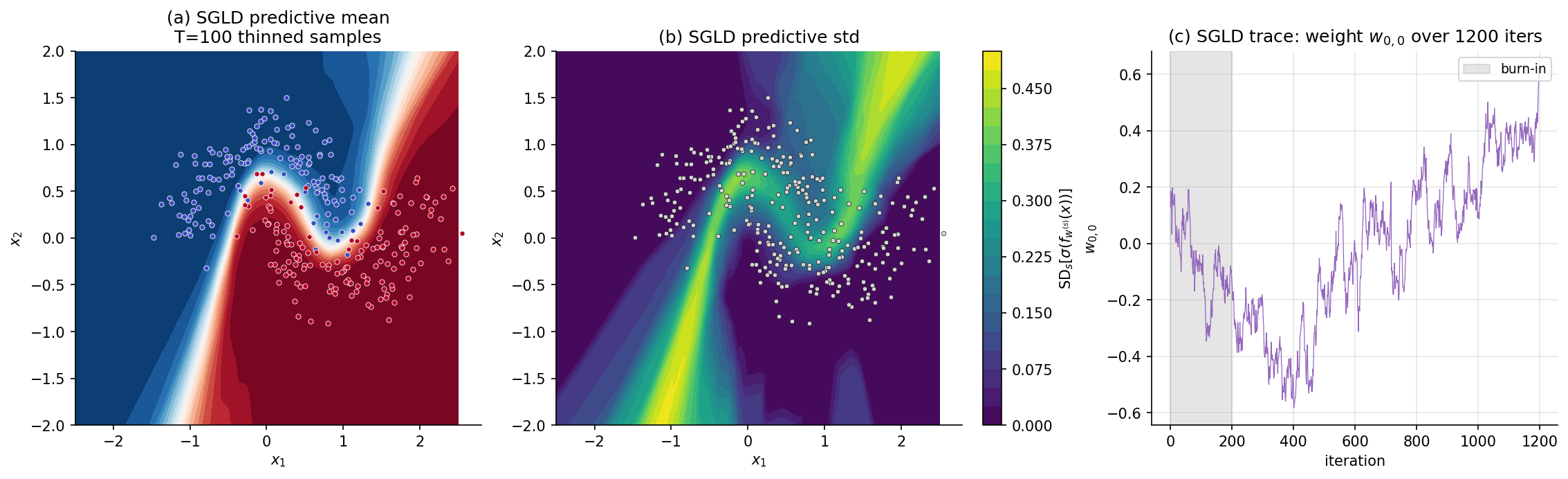
For the §6.7 Two Moons example we use constant $\eta = 10^{-3}$, mini-batch size $b = 32$, burn-in $T_{\mathrm{burn}} = 200$, sample count $T = 100$, thinning $\Delta = 10$ — total $200 + 100 \cdot 10 = 1200$ iterations, each iteration a single forward+backward pass on a $b = 32$ mini-batch. Total cell runtime ~7 s.

Loading…

7. Stochastic-gradient HMC (SGHMC)

SGLD’s mixing is rate-limited by the first-order Langevin diffusion: each step is a small drift along the gradient plus an isotropic Brownian kick, so traversing a long, low-curvature ridge in the loss landscape requires many small steps. Stochastic-gradient Hamiltonian Monte Carlo (SGHMC; Chen, Fox & Guestrin 2014) lifts the dynamics from first-order to second-order Langevin: introduce a momentum variable, let the chain accumulate velocity along the gradient, and damp the velocity with a friction term that simultaneously enforces stationarity and absorbs the variance contributed by stochastic gradients. Empirically the result mixes considerably faster than SGLD at the same wall-clock cost.

7.1 The second-order Langevin SDE

Augment the state with a momentum variable $v \in \mathbb{R}^p$ and let $M \in \mathbb{R}^{p \times p}$ be a positive-definite mass matrix (typically $M = I_p$). The underdamped Langevin SDE is $dw_t = M^{-1} v_t\,dt, \qquad dv_t = -\nabla U(w_t)\,dt - C\, M^{-1} v_t\,dt + \sqrt{2 C}\,dB_t,$ where $C \in \mathbb{R}^{p \times p}$ is a positive-semidefinite friction matrix. The Fokker–Planck calculation (analogous to §6.1) gives the stationary distribution $\pi(w, v) \;\propto\; \exp\!\Bigl(-U(w) - \tfrac{1}{2}\, v^\top M^{-1} v\Bigr),$ the joint posterior over $(w, v)$ in which the marginal $\pi(w) \propto e^{-U(w)} = p(w \mid \mathcal{D})$ is exactly the BNN posterior we want and the velocity is independent Gaussian noise we can discard. So the second-order Langevin SDE samples the posterior at higher mixing rate than SGLD because momentum carries the chain through low-curvature regions in many fewer steps.

7.2 The complication: stochastic gradients add variance to velocity

If we discretize the SDE via Euler–Maruyama with full-data gradients, we get a $w$-and-$v$ analogue of SGLD that converges to $\pi$ as the step size decays. But replacing $\nabla U$ with a stochastic mini-batch estimate $\hat g$ introduces an extra noise term in the velocity dynamics: $dv_{\mathrm{stoch}} = -\hat g\,dt - C M^{-1} v\,dt + \sqrt{2 C}\,dB \;=\; -\nabla U\,dt - \zeta\,dt - C M^{-1} v\,dt + \sqrt{2 C}\,dB,$ where $\zeta := \hat g - \nabla U$ is zero-mean stochastic-gradient noise with covariance $B(w) := \mathrm{Cov}[\hat g \mid w]$. The extra $\zeta$ term changes the effective noise covariance from $2C$ to $2C + B$, and the stationary distribution shifts away from $\pi$. Without correction, stochastic-gradient HMC samples a perturbed posterior. The Chen–Fox–Guestrin fix is the friction-compensation: choose the friction matrix $C$ large enough that the injected Brownian noise can absorb the gradient noise.

7.3 The SGHMC update

The structural reading: $(1 - \alpha)$ scales the previous velocity (friction damping), $-\eta \hat g_t$ accelerates along the negative gradient (Hamiltonian drift), and the Brownian-noise injection has scale $\sqrt{2\eta(C - \hat B)}$ — less than the $\sqrt{2\eta C}$ that the un-compensated SDE would inject, by exactly the right amount to absorb the additional variance the stochastic gradient contributes. When $\hat B = 0$ (the simplest practical choice — no covariance estimation), we use $\sqrt{2\eta C}$ noise injection and accept an $O(\eta)$ bias of the same order as constant-stepsize SGLD; when $\hat B$ is exact and $C \succeq B(w)$, the chain has the correct stationary distribution at any step size.

7.4 Stationary distribution

In practice $\hat B(w) = 0$ is the standard simplifying choice — the stochastic-gradient covariance is hard to estimate cheaply and depends on $w$. The resulting chain has $O(\eta)$ bias from the un-compensated gradient noise (Prop 7.3 below), of the same order as constant-stepsize SGLD’s bias, and the friction $C$ is tuned to be large enough that the bias is below the noise floor of downstream metrics.

7.5 Friction-vs-noise tradeoff

The Chen–Fox–Guestrin contribution, in summary: SGHMC at fixed $\eta$ has the same $O(\eta)$ bias as SGLD, but with the momentum-variable advantage that mixing is much faster — the chain explores the posterior in fewer iterations. For the same wall-clock budget, SGHMC typically produces a more accurate estimate of posterior expectations than SGLD, even at the cost of carrying the velocity variable through every iteration.

7.6 Practical preconditioning

7.7 Algorithm and worked example

Algorithm 7.5 (SGHMC posterior sampling).

Input: training data $\mathcal{D}$, network $f_w$, prior scale $\tau^2$, step size $\eta$, friction $C = c I_p$, mass $M = I_p$, mini-batch size $b$, burn-in $T_{\mathrm{burn}}$, sample count $T$, thinning interval $\Delta$. Output: posterior samples $w^{(1)}, \ldots, w^{(T)}$.

1. Initialize $w_0$ (random init or MAP warm-start), $v_0 = 0$.
2. For $t = 0, 1, \ldots, T_{\mathrm{burn}} + T \cdot \Delta$:
   • (a) Sample mini-batch $\mathcal{B}_t \subset \mathcal{D}$.
   • (b) Compute stochastic gradient $\hat g_t$ per Definition 6.1.
   • (c) Draw $\xi_t \sim \mathcal{N}(0, I_p)$.
   • (d) Update: $v_{t+1} \leftarrow (1 - \eta c) v_t - \eta\, \hat g_t + \sqrt{2 \eta c}\, \xi_t$; $\;w_{t+1} \leftarrow w_t + \eta\, v_{t+1}$.
3. Discard the first $T_{\mathrm{burn}}$ iterations as burn-in.
4. Return $w^{(s)} := w_{T_{\mathrm{burn}} + s\Delta}$ for $s = 1, \ldots, T$.

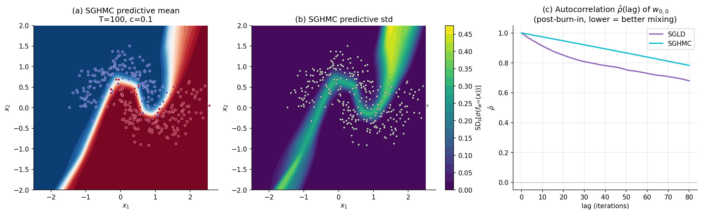
For the Two Moons example we use $\eta = 10^{-3}$, $c = 0.1$, $b = 32$, $T_{\mathrm{burn}} = 200$, $T = 100$, $\Delta = 10$ — same total iteration count as §6, exposing the head-to-head mixing comparison. Total cell runtime ~7 s.

Loading…

The §§6–7 development of SGLD and SGHMC stops at the recipes that work in practice. The deeper theory — the Itô-SDE view, the Fokker–Planck stationary-distribution proofs, the Vollmer–Zygalakis–Teh $O(\eta + 1/B)$ bias bound, Riemann-manifold preconditioning for hierarchical models, and a head-to-head with NUTS that pins down where SG-MCMC genuinely wins — is the subject of stochastic-gradient-mcmc.

8. Calibration and uncertainty quantification

§§3–7 each produce a predictive distribution. §1’s panel (c) and the per-section heatmaps make the qualitative claim that BNN methods produce sharper uncertainty in the right places, but qualitative is not enough — reading a predictive distribution responsibly requires knowing whether the reported probabilities match empirical frequencies. A model that confidently predicts “90% chance class 1” should be right on roughly $90\%$ of inputs that get that prediction; if it is right $70\%$ of the time, it is over-confident and downstream decisions made under those probabilities will be miscalibrated. This section develops three calibration metrics — expected calibration error, the Brier score, and negative log-likelihood — that quantify how well predictive probabilities match empirical reality, decomposes BNN predictive variance into epistemic and aleatoric components, and runs the four §§3–7 methods plus the §1 point estimate head-to-head on a held-out Two Moons test set. The cold-posterior effect (Wenzel et al. 2020) and post-hoc temperature scaling (Guo et al. 2017) get their own remarks at the end.

8.1 Expected calibration error

The simplest calibration metric. Bin the test predictions by predicted probability into $B$ bins of equal width on $[0, 1]$, and compare in-bin accuracy to in-bin average confidence.

A perfectly-calibrated model has $\mathrm{ECE} = 0$: in every bin, the empirical accuracy matches the average confidence. ECE is always non-negative. Standard practice uses $B = 10$ or $B = 15$ bins; results are not very sensitive to $B$ for $N \geq 10^3$. ECE has a known weakness — it does not reward sharp predictions when accuracy is bin-averaged — but its interpretability (it has units of “probability points off”) makes it the most-reported calibration metric in the BNN literature.

8.2 The Brier score

A strictly proper scoring rule for binary classification. Where ECE is bin-based, Brier is point-wise: it averages the squared error between predicted probability and binary outcome.

The decomposition reads: BS = (how miscalibrated within bins) − (how varied accuracy is across bins) + (irreducible class-base-rate variance). Uncertainty is the “no-skill” baseline; Resolution rewards a model whose accuracy varies meaningfully across bins; Reliability is the calibration-error analog of ECE. A perfectly calibrated model has Reliability = 0; a fully-discriminating model has Resolution = Uncertainty.

8.3 Negative log-likelihood

NLL has two practical properties that ECE and Brier do not. It penalizes over-confident wrong predictions most aggressively: $-\log p$ blows up as $p \to 0$ for the true class. And it directly compares to held-out log-likelihoods used elsewhere in Bayesian model selection — the BIC, the marginal likelihood, the WAIC, and the LOO predictive log-density all share NLL’s units (nats per observation). For BNN inference, NLL is usually the headline metric, with ECE and Brier as complementary diagnostics.

8.4 The epistemic-aleatoric decomposition

A BNN’s predictive variance decomposes into two pieces — what the model would learn from more data versus what no model can ever learn — and the decomposition is exactly the law of total variance applied to the BNN predictive.

Practically, the epistemic term is what BNN methods compute via Monte Carlo: the §3, §4, §5, §6, §7 predictive standard-deviation heatmaps are $\sqrt{\text{epistemic variance}}$. The aleatoric term is the average over weight samples of the per-sample conditional variance — for a Bernoulli observation, this is the sigmoid-of-logit variance and is large near the decision boundary regardless of how confident the model is in its weights. The §8.7 head-to-head figure renders both components separately for one method (deep ensemble) so the reader can see the decomposition concretely.

8.5 The cold-posterior effect

8.6 Temperature scaling

8.7 Head-to-head comparison

Algorithm 8.7 (Head-to-head calibration evaluation).

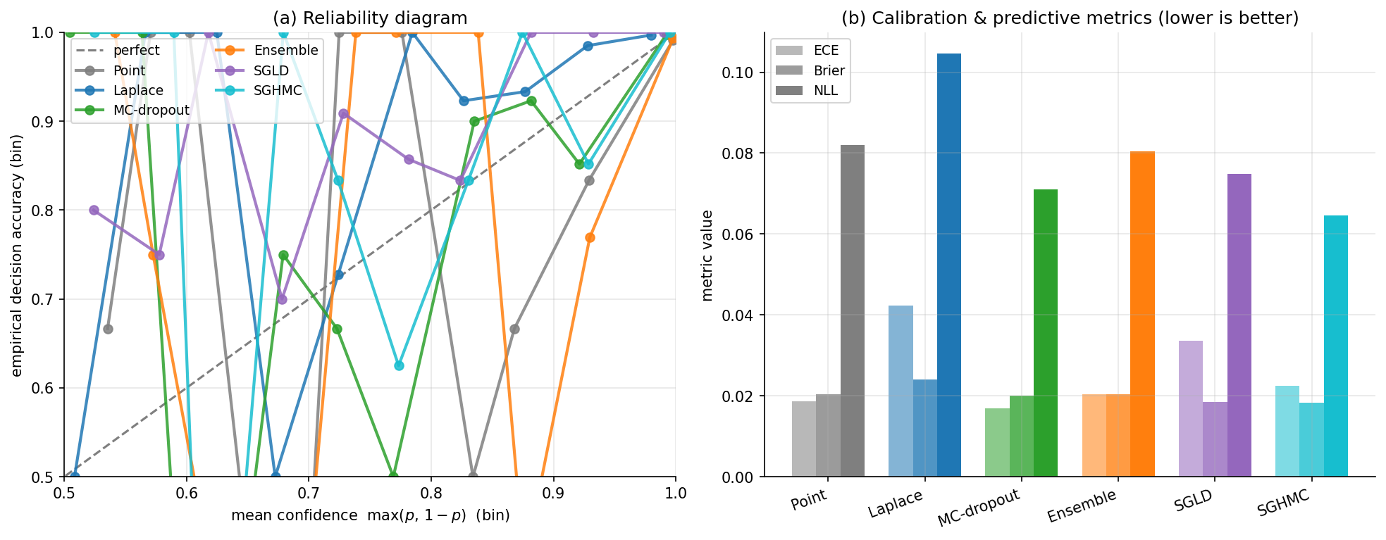
Input: training data $\mathcal{D}$, held-out test set $\mathcal{D}_{\mathrm{test}} = \{(x^*_i, y^*_i)\}_{i=1}^{N_{\mathrm{test}}}$, the six method outputs from §§1, 3, 4, 5, 6, 7 (point estimate, Laplace, MC-dropout, deep ensemble, SGLD, SGHMC). Output: table of $\{\mathrm{ECE}, \mathrm{BS}, \mathrm{NLL}\}$ for each method, with reliability diagrams.

1. For each method $m$, compute predicted class-1 probabilities $\hat{p}^{(m)}_i$ on the test set via Monte Carlo over the method’s posterior samples.
2. Compute ECE with $B = 10$ bins, BS via Def 8.2, NLL via Def 8.3.
3. Plot reliability diagrams: predicted-confidence bin centers on $x$-axis, $\mathrm{acc}(b)$ on $y$-axis, with the diagonal $y = x$ marked as the perfectly-calibrated reference.

For Two Moons we use $N_{\mathrm{test}} = 500$ held-out points generated with make_moons at the same noise level as training but a different random_state, so the test set is iid from the same distribution as training and ECE is well-defined.

9. Function-space view: NNGP, NTK, and open problems

§§3–7 work in weight space. Each method approximates the posterior $p(w \mid \mathcal{D})$ over the network’s parameters and reads predictions off the resulting weight distribution. The §2.4 obstacles — multimodality, ReLU rescaling, over-parametrization — are all weight-space pathologies, and the methods of §§3–7 are weight-space workarounds. Function space offers a different vantage. What we ultimately care about is the predictive distribution over outputs, which lives in function space; weight space is the awkward intermediate representation. Two classical results — Neal’s 1996 neural network Gaussian process (NNGP) and Jacot, Gabriel & Hongler’s 2018 neural tangent kernel (NTK) — show that in the infinite-width limit, both Bayesian inference and gradient-descent training reduce to operations on a fixed kernel function. The function-space view connects BNNs to Gaussian Processes, explains why deep ensembles work, and provides the asymptotic reference against which the §§3–7 methods can be evaluated. This section gives the four key facts, with proofs deferred to references; the running example is one panel of NNGP-prior samples that visualizes the infinite-width convergence.

9.1 The neural network Gaussian process

Neal’s 1996 PhD thesis proved the one-hidden-layer case via a direct CLT argument: each output $f_w(x) = \sum_j w^{(2)}_j \phi(W^{(1)}_j x + b^{(1)}_j)$ is a sum of $h_1$ iid bounded random variables (in the sense that suitable moments are bounded), so the CLT applies and $f_w(x)$ converges to a Gaussian. Joint distributions across multiple inputs $x_1, \ldots, x_n$ likewise converge to a multivariate Gaussian — i.e., a Gaussian process. Lee et al. 2017 extended the argument to deep networks via induction over layers, giving the recursive kernel formula above.

The implication is structural: at infinite width, BNN posterior inference reduces to GP regression (or GP classification, via Laplace or EP, per Gaussian Processes). The NNGP kernel encodes the entire architectural choice — depth, activation, prior scales — and once the kernel is in hand the $O(n^3)$ GP-inference machinery applies directly. There is no weight-space optimization, no MAP, no Hessian, no SGLD. The infinite-width BNN is a Gaussian process.

9.2 The neural tangent kernel

Jacot et al.’s argument has two parts. First, at initialization, the gradient $\nabla_w f_{w_0}(x)$ is itself a random function whose pairwise inner products converge in the infinite-width limit to a deterministic kernel $\Theta_*$ — a CLT analogous to NNGP’s. Second, during training, the change in weights $w_t - w_0$ stays small in a width-dependent norm (the lazy regime of Chizat & Bach 2019), so the linearization $f_w(x) \approx f_{w_0}(x) + \nabla_w f_{w_0}(x)^\top (w - w_0)$ remains valid and the network’s outputs evolve linearly. The combination gives kernel-regression dynamics in function space.

The NTK is not the same as the NNGP kernel. NNGP describes the prior over functions before any training; NTK describes the trained function under gradient descent. In general $\Theta_{\mathrm{NTK}}(x, x') \neq k_{\mathrm{NNGP}}(x, x')$, and at infinite width they describe two different inference regimes (Bayesian posterior vs. gradient-descent training). Lee et al. 2019 (“Wide Neural Networks of Any Depth Evolve as Linear Models Under Gradient Descent”) gave the precise statement of NTK convergence and the relationship between the two kernels.

9.3 What this means for the §§3–7 methods

The §8 head-to-head ordering on Two Moons is roughly consistent with this asymptotic ordering: deep ensembles and SG-MCMC are the most-calibrated, Laplace is in the middle, and MC-dropout is at the bottom. For finite-width networks the differences are smaller than the infinite-width view suggests, and for some narrow regimes the ordering inverts — but the function-space asymptotic gives the right intuition for which method to reach for first.

9.4 Open problems

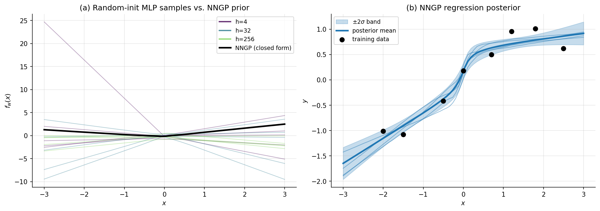
Connections and further reading

The function-space view connects this topic to neighboring formalML topics. Gaussian Processes develops the GP machinery the NNGP relies on — Cholesky factorization of the kernel matrix, conditional-MVN posteriors, hyperparameter learning by marginal likelihood. Variational Inference is the substrate for §4’s MC-dropout derivation and for the planned function-space VI of Rem 9.4. Stacking & Predictive Ensembles generalizes §5’s uniform-weighted deep ensemble to learned weights. Stochastic-Gradient MCMC and the planned meta-learning build directly on §§6–7’s SG-MCMC machinery; Sparse Bayesian Priors revisits §2.1’s prior choice with heavy-tailed alternatives that resolve some of Rem 9.4’s cold-posterior questions. Cross-site, formalstatistics’s formalStatistics: Bayesian Foundations and Prior Selection provides the prior-and-likelihood machinery this topic takes as given, and formalStatistics: Central Limit Theorem is the rigorous source of the Bernstein–von Mises invocation in §2.3.