KL Divergence & f-Divergences

Overview & Motivation

Cross-entropy loss, variational inference, and generative adversarial networks look like three unrelated ideas. But they share a common engine: each one minimizes a divergence — a function that measures how one probability distribution differs from another.

• Cross-entropy loss minimizes the KL divergence from the true label distribution to the model’s predictions (forward KL).
• Variational inference minimizes the KL divergence from an approximate posterior to the true posterior (reverse KL), which is equivalent to maximizing the ELBO.
• GANs minimize the Jensen–Shannon divergence between the real data distribution and the generator’s output.

All three are special cases of f-divergence minimization, a framework that unifies a family of distributional distance measures through convex analysis. Understanding this framework gives us a single lens through which cross-entropy loss, the ELBO, and the GAN objective are all the same idea in different clothes.

This topic develops the theory systematically: we start with KL divergence and its operational meaning as the excess cost of miscoding, then explore how the direction of the KL divergence (forward vs reverse) determines fundamentally different fitting behavior. We generalize to f-divergences — showing that KL, reverse KL, $\chi^2$, Hellinger, total variation, and Jensen–Shannon are all members of one family parameterized by convex generator functions. Variational representations via Fenchel conjugates turn these abstract measures into optimization problems that can be solved with neural networks. Rényi divergences provide a complementary one-parameter family with applications to differential privacy and hypothesis testing.

Prerequisites

This topic builds on:

• Shannon Entropy & Mutual Information — KL divergence is defined as the gap between cross-entropy and entropy: $D_{\mathrm{KL}}(p \| q) = H(p, q) - H(p)$. We use entropy, mutual information, and the data processing inequality throughout.

What We Cover

1. KL divergence — definition, Gibbs’ inequality, asymmetry, cross-entropy decomposition
2. Forward vs reverse KL — mode-covering vs mode-seeking, connections to MLE and variational inference
3. f-divergences — the unifying framework via convex generator functions
4. Properties of f-divergences — non-negativity, joint convexity, data processing inequality, Pinsker’s inequality
5. Variational representations — Fenchel conjugates, Donsker–Varadhan, NWJ bound, connection to GANs
6. Rényi divergence — the $\alpha$-divergence family, monotonicity, special cases
7. Computational notes — estimation, cross-entropy loss, ELBO, practical implementations

---

KL Divergence: Definition & Properties

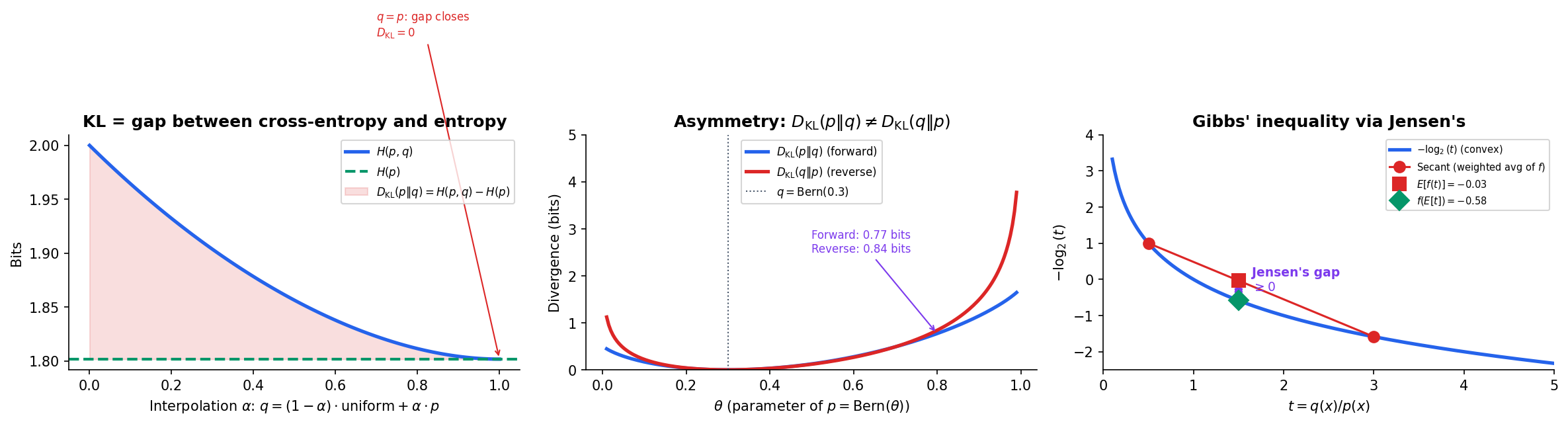
In Shannon Entropy & Mutual Information, we defined the entropy $H(p)$ as the minimum average code length for a source with distribution $p$. If we use a code optimized for a different distribution $q$, the average code length increases to $H(p, q) = -\sum_x p(x) \log_2 q(x)$ — the cross-entropy. The difference is the excess cost of using the wrong code.

The operational meaning: $D_{\mathrm{KL}}(p \| q)$ is the expected number of extra bits needed to encode samples from $p$ using a code optimized for $q$, beyond the minimum achieved by the optimal code for $p$.

The key decomposition connecting these quantities is immediate:

Gibbs’ Inequality

The most fundamental property of KL divergence is non-negativity: using the wrong code never helps.

Asymmetry

Unlike a true distance, KL divergence is not symmetric.

Counterexample. Let $p = (0.9, 0.1)$ and $q = (0.5, 0.5)$. Then:

$D_{\mathrm{KL}}(p \| q) = 0.9 \log_2 \frac{0.9}{0.5} + 0.1 \log_2 \frac{0.1}{0.5} \approx 0.368 \text{ bits}$

$D_{\mathrm{KL}}(q \| p) = 0.5 \log_2 \frac{0.5}{0.9} + 0.5 \log_2 \frac{0.5}{0.1} \approx 0.795 \text{ bits}$

The asymmetry is not a defect — it encodes fundamentally different information about the relationship between $p$ and $q$. The direction you choose determines the fitting behavior, as we explore in the next section.

KL divergence is also not a metric: it violates the triangle inequality. It is not even a semimetric (which requires symmetry). Despite this, it plays a central role because its information-theoretic interpretation is exact and its connection to maximum likelihood estimation is direct.

Explore the interactive visualization below. Drag the bars to adjust both distributions and watch the KL divergence, cross-entropy, and their asymmetry update in real time.

Outcomes k:2346Match (q = p)Uniform qDrag bars to adjust p (blue) and q (red)

import numpy as np

def kl_divergence(p, q):
    """KL divergence D_KL(p || q) in bits."""
    p, q = np.asarray(p, float), np.asarray(q, float)
    mask = p > 0
    if np.any(q[mask] <= 0):
        return np.inf
    return np.sum(p[mask] * np.log2(p[mask] / q[mask]))

def cross_entropy(p, q):
    """Cross-entropy H(p, q) in bits."""
    p, q = np.asarray(p, float), np.asarray(q, float)
    mask = p > 0
    if np.any(q[mask] <= 0):
        return np.inf
    return -np.sum(p[mask] * np.log2(q[mask]))

# Cross-entropy decomposition: H(p, q) = H(p) + D_KL(p || q)
p = np.array([0.4, 0.35, 0.15, 0.1])
q = np.array([0.25, 0.25, 0.25, 0.25])

H_p = -np.sum(p * np.log2(p))              # 1.8464 bits
H_pq = cross_entropy(p, q)                  # 2.0000 bits
D_KL = kl_divergence(p, q)                  # 0.1536 bits
# Verify: H_pq ≈ H_p + D_KL → 2.0000 ≈ 1.8464 + 0.1536 ✓

---

Forward vs Reverse KL

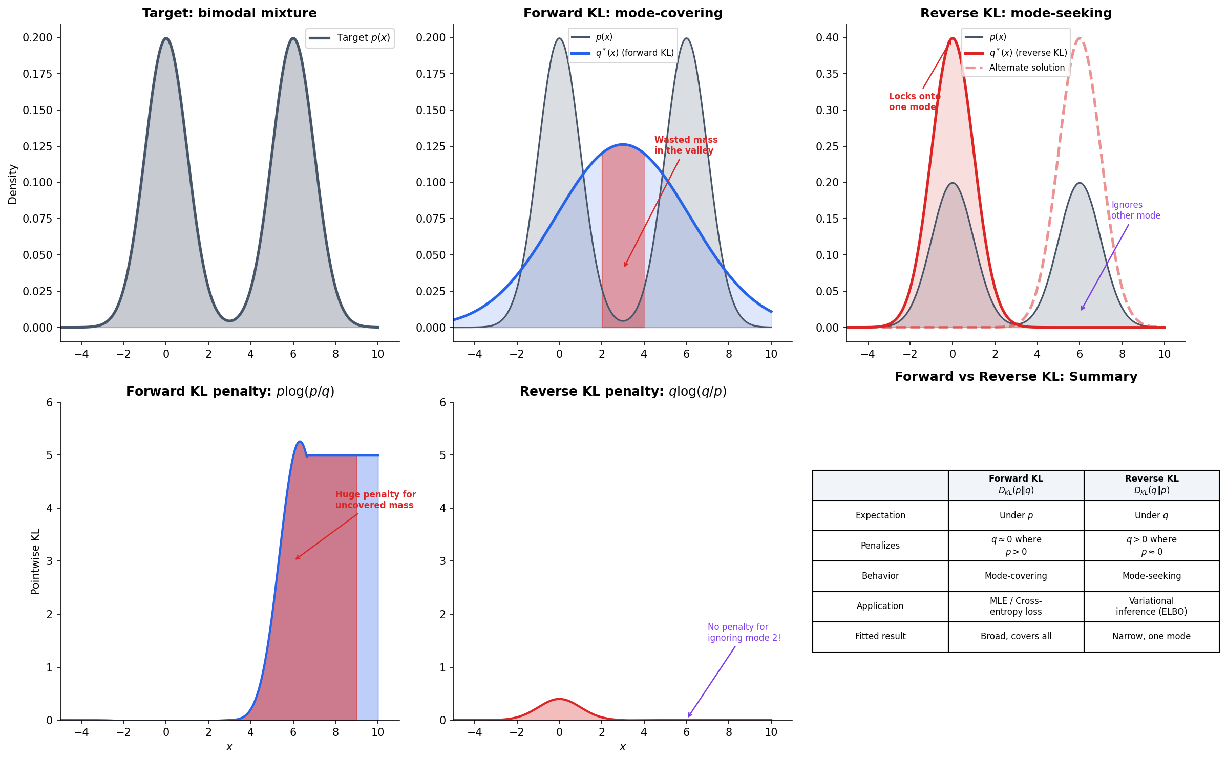
The asymmetry of KL divergence is not merely a mathematical curiosity — it produces two fundamentally different fitting behaviors. When we approximate a complex distribution $p$ with a simpler model $q$, the direction of the KL divergence we minimize determines what kind of approximation we get.

Forward KL: Mode-Covering

Minimizing forward KL $D_{\mathrm{KL}}(p \| q)$ over the model family $\{q_\theta\}$ produces a model that covers all modes of $p$.

$\min_\theta D_{\mathrm{KL}}(p \| q_\theta) = \min_\theta \mathbb{E}_p\!\left[\log \frac{p(X)}{q_\theta(X)}\right] = \min_\theta \left[-\mathbb{E}_p[\log q_\theta(X)]\right] + \text{const}$

The penalty comes from $p(x) \log(p(x)/q(x))$: if $p(x) > 0$ but $q(x) \approx 0$, the term $\log(p(x)/q(x)) \to +\infty$. This penalty forces $q$ to place mass everywhere $p$ does — it must cover all modes, even at the cost of putting wasted probability mass in regions between modes.

Reverse KL: Mode-Seeking

Minimizing reverse KL $D_{\mathrm{KL}}(q \| p)$ produces a model that seeks a single mode of $p$.

$\min_\theta D_{\mathrm{KL}}(q_\theta \| p) = \min_\theta \mathbb{E}_{q_\theta}\!\left[\log \frac{q_\theta(X)}{p(X)}\right]$

Now the penalty comes from $q(x) \log(q(x)/p(x))$: if $p(x) \approx 0$ but $q(x) > 0$, the term explodes. This forces $q$ to avoid placing mass where $p$ does not — but it has no penalty for ignoring modes of $p$ where $q$ is already zero. The result: $q$ locks onto a single mode and ignores the rest.

The visualization below demonstrates this contrast on a bimodal target. A single Gaussian fit under forward KL spreads to cover both peaks (with wasted mass in the valley), while under reverse KL it locks onto one peak.

Mode separation:4σTarget:Bimodal symmetricBimodal asymmetricTrimodalFit: single Gaussian

---

f-Divergences: A Unifying Framework

KL divergence is one member of a much larger family. Ali & Silvey (1966) and Csiszár (1967) independently showed that a single construction — parameterized by a convex function — generates an entire family of divergences, all sharing the key properties we proved for KL.

The generator function $f$ determines which divergence we get. Every $f$ satisfying the conditions above — convex, with $f(1) = 0$ — produces a valid divergence that is non-negative and zero iff $p = q$.

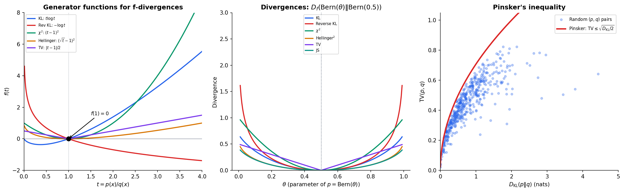
The following table shows six important special cases, each recoverable by choosing the appropriate generator:

• KL divergence: $f(t) = t \log t$ gives $\sum p(x) \log(p(x)/q(x))$
• Reverse KL: $f(t) = -\log t$ gives $\sum q(x) \log(q(x)/p(x))$
• $\chi^2$ divergence: $f(t) = (t - 1)^2$ gives $\sum (p(x) - q(x))^2/q(x)$
• Squared Hellinger: $f(t) = (\sqrt{t} - 1)^2$ gives $\sum (\sqrt{p(x)} - \sqrt{q(x)})^2$
• Total variation: $f(t) = |t - 1|/2$ gives $\frac{1}{2}\sum |p(x) - q(x)|$
• Jensen–Shannon: $f(t) = t \log\frac{2t}{t+1} + \log\frac{2}{t+1}$ gives $\frac{1}{2}D_{\mathrm{KL}}(p \| m) + \frac{1}{2}D_{\mathrm{KL}}(q \| m)$

where $m = (p + q)/2$ in the Jensen–Shannon case.

Explore the f-divergence family below. The left panel shows the generator functions — all convex, all passing through $(1, 0)$. The right panel shows how each divergence responds to distributional mismatch.

KLReverse KLχ²Hellinger²TVJensen–ShannonPinsker k:3510

def f_divergence(p, q, f_func):
    """General f-divergence D_f(p || q) = sum q(x) f(p(x)/q(x))."""
    p, q = np.asarray(p, float), np.asarray(q, float)
    result = 0.0
    for pi, qi in zip(p, q):
        if qi > 0 and pi > 0:
            result += qi * f_func(pi / qi)
        elif qi > 0 and pi == 0:
            result += qi * f_func(0.0)
        elif qi == 0 and pi > 0:
            return np.inf
    return result

# Generator functions (use natural log — the standard convention for
# f-divergences; kl_divergence() above uses log2 for bits)
f_kl         = lambda t: t * np.log(t) if t > 0 else 0.0
f_reverse_kl = lambda t: -np.log(t) if t > 0 else np.inf
f_chi_sq     = lambda t: (t - 1) ** 2
f_hellinger  = lambda t: (np.sqrt(max(t, 0)) - 1) ** 2
f_tv         = lambda t: abs(t - 1) / 2
f_js         = lambda t: (t * np.log(t / ((t + 1) / 2)) + np.log(1 / ((t + 1) / 2))
                          if t > 0 else np.log(2))

---

Properties of f-Divergences

The power of the f-divergence framework is that all members inherit fundamental properties from the convexity of $f$ alone. We do not need separate proofs for KL, $\chi^2$, Hellinger, etc. — one proof covers them all.

This is the same proof structure as Gibbs’ inequality for KL — because Gibbs’ inequality is the special case $f(t) = t \log t$.

Joint convexity means that divergence minimization — minimizing $D_f(p \| q_\theta)$ over parameters $\theta$ — is a convex problem when the mapping $\theta \mapsto q_\theta$ is affine.

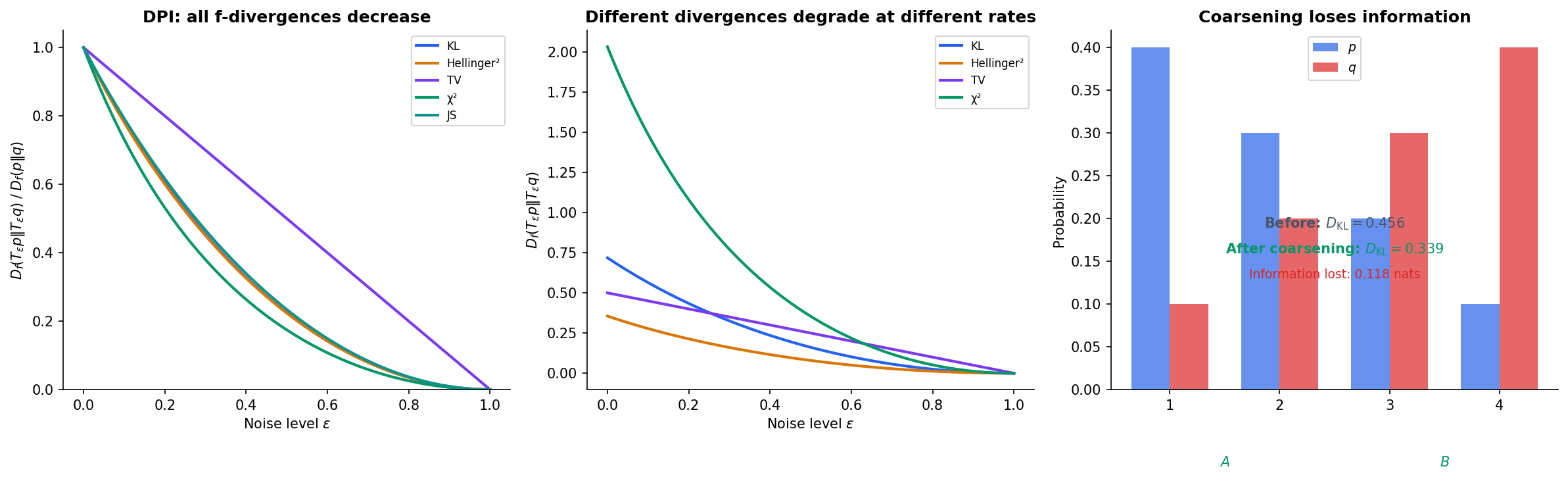
Data Processing Inequality for f-Divergences

The data processing inequality (DPI) says that processing data can only lose information — it can never increase the divergence between two distributions.

This is strictly more general than the mutual information DPI from Shannon Entropy & Mutual Information. The mutual information DPI $I(X; Z) \leq I(X; Y)$ for a Markov chain $X \to Y \to Z$ is the special case where $D_f = D_{\mathrm{KL}}$ applied to the joint vs product of marginals.

Pinsker’s Inequality

Pinsker’s inequality provides a bridge between KL divergence and total variation — two divergences with very different structures.

The proof involves a careful comparison of the generator functions for TV and KL via a quadratic bound on $t \log t$ near $t = 1$ (see Cover & Thomas, Ch. 11, or Tsybakov, 2009). The bound is tight: equality is approached as $p$ and $q$ become close.

Pinsker’s inequality is practically important: total variation has a clean interpretation (maximum probability difference over events) but is hard to work with in optimization; KL divergence has a clean optimization theory (convexity, connections to MLE) but a less transparent geometric interpretation. Pinsker’s inequality lets us convert bounds between them.

---

Variational Representations

The variational representation of f-divergences is one of the most powerful results in modern information theory. It transforms divergence computation from a density ratio problem (requiring knowledge of $p$ and $q$) into an optimization problem (requiring only samples from $p$ and $q$).

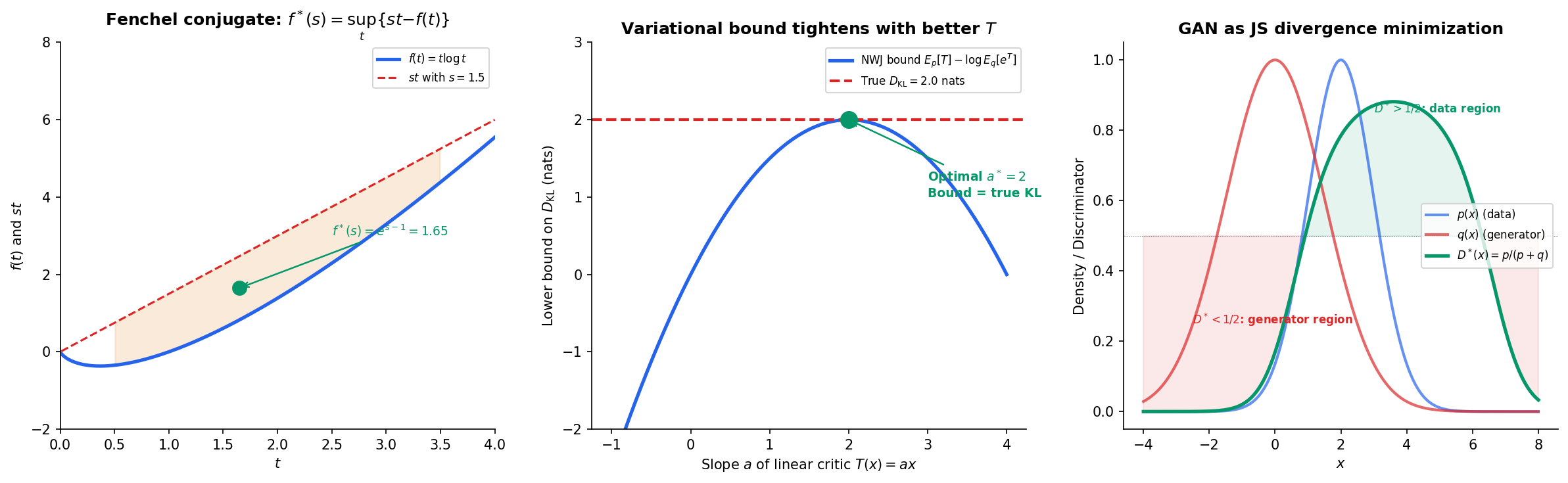
The key idea comes from Convex Analysis: every convex function can be represented as the supremum of affine functions via its Fenchel conjugate (also called the convex conjugate or Legendre transform):

$f^*(s) = \sup_{t > 0}\{st - f(t)\}$

Donsker–Varadhan and NWJ Bounds

For KL divergence specifically, $f(t) = t \log t$ gives $f^*(s) = e^{s-1}$, yielding:

The Nguyen–Wainwright–Jordan (NWJ) bound is a related lower bound that replaces $\log \mathbb{E}_q[e^T]$ with $\mathbb{E}_q[e^{T-1}]$, which is easier to optimize:

$D_{\mathrm{KL}}(p \| q) \geq \sup_T \left\{\mathbb{E}_p[T(X)] - \mathbb{E}_q[e^{T(X) - 1}]\right\}$

Connection to GANs

Slope s:1.5μ_p (mean of p):2.0

---

Rényi Divergence & $\alpha$-Divergences

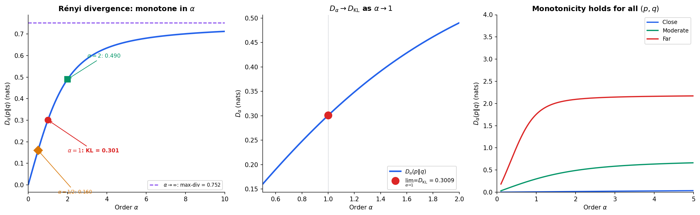
The f-divergence family is parameterized by a function. Rényi divergences provide a complementary parameterization by a single scalar $\alpha$, interpolating between familiar divergences.

The Rényi family provides a continuous spectrum of divergences. As $\alpha$ varies, we recover fundamental information-theoretic quantities:

• $\alpha \to 0$: $-\log q(\text{supp}(p))$ — support divergence
• $\alpha = 1/2$: $-2\log\sum_x \sqrt{p(x)q(x)}$ — Bhattacharyya distance
• $\alpha \to 1$: $D_{\mathrm{KL}}(p \| q)$ — KL divergence (by L’Hôpital)
• $\alpha = 2$: $\log\sum_x p(x)^2/q(x)$ — related to $\chi^2$ divergence
• $\alpha \to \infty$: $\log\max_x p(x)/q(x)$ — max-divergence

The convergence $D_\alpha \to D_{\mathrm{KL}}$ as $\alpha \to 1$ is verified by L’Hôpital’s rule applied to the $0/0$ indeterminate form in the definition.

This monotonicity has important consequences:

• Differential privacy: The $(\varepsilon, \delta)$-DP guarantee is controlled by the max-divergence ($\alpha = \infty$). Rényi DP (Mironov, 2017) uses finite $\alpha$ to get tighter composition bounds, leveraging the monotonicity to relate different privacy definitions.
• Hypothesis testing: The Chernoff information, which governs the optimal Bayesian error exponent, is $\min_\alpha D_\alpha(p \| q)$.

def renyi_divergence(p, q, alpha):
    """Rényi divergence D_alpha(p || q) in nats."""
    p, q = np.asarray(p, float), np.asarray(q, float)
    if abs(alpha - 1.0) < 1e-10:
        # Limit: KL divergence in nats
        mask = p > 0
        if np.any(q[mask] <= 0):
            return np.inf
        return np.sum(p[mask] * np.log(p[mask] / q[mask]))
    summand = np.sum(p ** alpha * q ** (1 - alpha))
    if summand <= 0:
        return np.inf
    return np.log(summand) / (alpha - 1)

# Verify: D_alpha → D_KL as alpha → 1
p = np.array([0.7, 0.2, 0.1])
q = np.array([0.3, 0.4, 0.3])
alphas = [0.5, 0.9, 0.99, 0.999, 1.0, 1.001, 1.01, 1.1, 2.0]
for a in alphas:
    print(f"D_{a:.3f}(p || q) = {renyi_divergence(p, q, a):.6f} nats")
# Observe smooth convergence to D_KL at α = 1

---

Computational Notes

Plug-In Estimation from Samples

Given i.i.d. samples from $p$ and $q$, the simplest KL estimator replaces the true distributions with empirical histograms:

$\hat{D}_{\mathrm{KL}}(\hat{p} \| \hat{q}) = \sum_x \hat{p}(x) \log_2 \frac{\hat{p}(x)}{\hat{q}(x)}$

This plug-in estimator is consistent but converges slowly — $O(1/\sqrt{n})$ in general — and is biased in finite samples due to the nonlinearity of $\log$. For continuous distributions, binning introduces discretization error, and kernel-based or $k$-NN estimators (Pérez-Cruz, 2008; Wang et al., 2009) are preferred.

Cross-Entropy Loss Decomposition

During training of a classifier with model $q_\theta$ and true distribution $p$:

$H(p, q_\theta) = H(p) + D_{\mathrm{KL}}(p \| q_\theta)$

The entropy $H(p)$ is the irreducible noise floor — we cannot reduce the loss below $H(p)$ no matter how good the model. The KL divergence $D_{\mathrm{KL}}(p \| q_\theta)$ is the reducible component that training shrinks toward zero. For one-hot labels, $H(p) = 0$ and cross-entropy equals KL divergence.

ELBO as Reverse KL

The evidence lower bound (ELBO) in variational inference decomposes as:

$\text{ELBO}(q_\phi) = \log p(x) - D_{\mathrm{KL}}(q_\phi(z) \| p(z|x))$

Since $\log p(x)$ is fixed, maximizing the ELBO is equivalent to minimizing the reverse KL to the posterior. The gap between $\log p(x)$ and the ELBO is exactly the reverse KL divergence — a direct measure of how well the approximate posterior fits the true posterior.

Practical Implementations

from scipy.special import rel_entr
import torch
import torch.nn.functional as F

# SciPy: KL divergence via relative entropy
# rel_entr(p, q) returns p * log(p/q) elementwise (in nats)
p = np.array([0.4, 0.35, 0.15, 0.1])
q = np.array([0.25, 0.25, 0.25, 0.25])
kl_nats = np.sum(rel_entr(p, q))  # D_KL in nats

# PyTorch: cross-entropy loss (forward KL for one-hot labels)
logits = torch.tensor([2.0, 1.0, 0.5, -0.5])
target = torch.tensor(0)  # one-hot: class 0
ce_loss = F.cross_entropy(logits, target)  # -log(softmax(logits)[0])

# PyTorch: KL divergence (expects log-probabilities for input)
log_q = F.log_softmax(logits, dim=0)
p_tensor = torch.tensor([0.4, 0.35, 0.15, 0.1])
kl = F.kl_div(log_q, p_tensor, reduction='sum')  # D_KL(p || q) in nats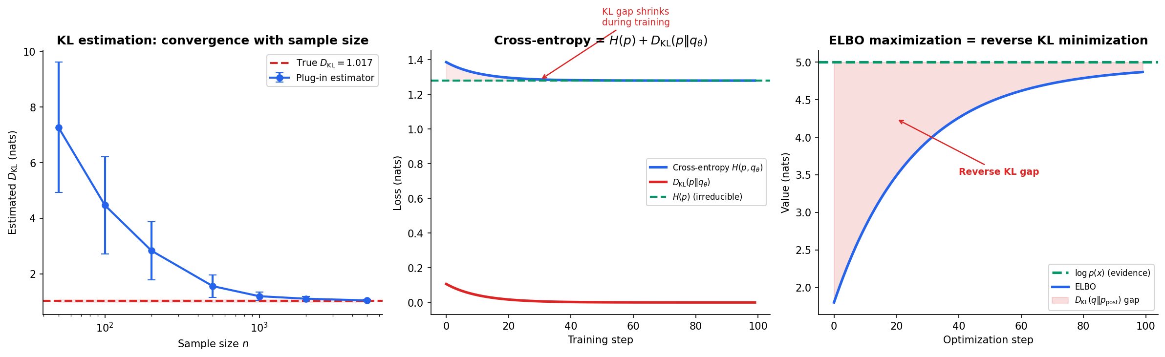

---

Connections & Further Reading

KL divergence and its generalizations connect information theory to optimization, geometry, and learning theory. This topic sits at the intersection of several curriculum tracks:

• Shannon Entropy & Mutual Information (Information Theory) — KL divergence decomposes as $D_{\mathrm{KL}}(p \| q) = H(p,q) - H(p)$. Mutual information $I(X;Y) = D_{\mathrm{KL}}(p_{XY} \| p_X p_Y)$. The data processing inequality for mutual information is a special case of the f-divergence DPI.

• Information Geometry & Fisher Metric (Differential Geometry) — The Fisher information matrix is the Hessian of KL divergence at $p = q$. The dual $e$- and $m$-connections arise from the asymmetry of KL. The $\alpha$-connections generalize via Rényi divergences.

• Convex Analysis (Optimization) — f-divergences are defined through convex generators; the Fenchel conjugate $f^*$ yields the variational representation; joint convexity makes divergence minimization a convex program.

• Measure-Theoretic Probability (Probability & Statistics) — Continuous KL requires the Radon–Nikodym derivative. Absolute continuity ($P \ll Q$) is necessary for finite KL divergence.

Downstream on this track

• Rate-Distortion Theory — the minimum rate $R(D)$ for encoding a source at distortion level $D$ is an optimization over mutual information — itself a KL divergence — subject to a distortion constraint. The Blahut–Arimoto algorithm iteratively minimizes KL divergence to compute $R(D)$.
• Minimum Description Length — model selection via code length: the regret of a universal code is bounded by the KL divergence between the true and estimated distributions. The minimax regret connects to the capacity of the model class.

Notation Reference

• $D_{\mathrm{KL}}(p \| q)$ — KL divergence from $p$ to $q$
• $H(p, q)$ — Cross-entropy from $p$ to $q$
• $D_f(p \| q)$ — f-divergence with generator $f$
• $f^*(s) = \sup_t\{st - f(t)\}$ — Fenchel conjugate of $f$
• $\mathrm{TV}(p, q)$ — Total variation distance
• $\mathrm{JS}(p \| q)$ — Jensen–Shannon divergence
• $D_\alpha(p \| q)$ — Rényi divergence of order $\alpha$