Shannon Entropy & Mutual Information
Information content, entropy, and mutual information — the quantities that measure uncertainty, surprise, and statistical dependence
Overview & Motivation
How much information does a random variable carry? How many bits do we need, at minimum, to encode a message? When two variables are statistically dependent, how much does knowing one tell us about the other?
These questions have precise, quantitative answers — and they all flow from a single idea that Claude Shannon published in 1948: entropy. Shannon showed that the uncertainty in a random variable has a unique, canonical measure, and that this measure controls the fundamental limits of data compression, communication, and statistical inference.
For machine learning, information theory is not optional background. Cross-entropy loss — the default objective for classification — is an information-theoretic quantity. Mutual information drives feature selection. The data processing inequality explains why deep representations can lose but never create information about the input. The maximum-entropy principle connects to Bayesian inference through the choice of priors. And KL Divergence & f-Divergences, the next topic on this track, builds directly on the entropy framework we develop here.
What We Cover
- Information content and Shannon entropy — the surprise of an outcome and the average surprise of a distribution
- Joint and conditional entropy — uncertainty in pairs of variables and the chain rule
- Mutual information — the symmetric measure of statistical dependence
- The data processing inequality — why post-processing cannot create information
- Differential entropy — the continuous extension and the maximum-entropy role of the Gaussian
- Source coding and compression — Shannon’s theorem, Kraft’s inequality, and Huffman coding
- Entropy rate — entropy for stochastic processes and Markov chains
- Connections to ML — cross-entropy loss, MI feature selection, and the InfoMax principle
Prerequisites
This topic builds on:
- Measure-Theoretic Probability — entropy is defined as the expectation , differential entropy requires the Lebesgue integral, and conditional entropy uses conditional expectation
Information Content & Shannon Entropy
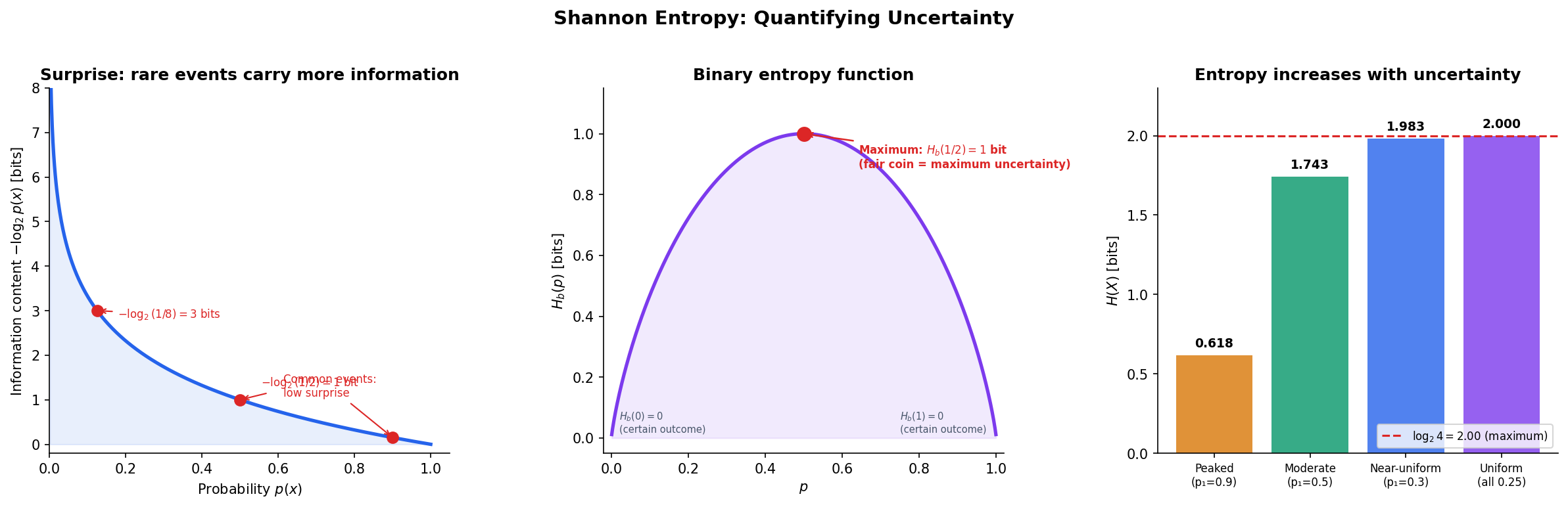
Imagine playing a guessing game. Your friend picks a card from a deck and you must guess which one. If the deck has 2 cards, one guess suffices — that’s 1 bit of uncertainty. A deck of 8 cards takes 3 guesses in the worst case — 3 bits. The pattern is clear: the uncertainty in a uniform draw over outcomes is bits.
But what if the outcomes are not equally likely? Shannon’s key insight was to define the information content (or surprise) of a single outcome, and then take the average to get the entropy.
Definition 1 (Information Content (Surprise)).
The information content (or self-information) of an outcome with probability is
An outcome with probability carries bit of information. An outcome with probability carries bits. Common events carry little surprise; rare events carry a lot.
The choice of gives units of bits. Using gives nats; using gives hartleys. The choice of base is a convention — we use bits throughout this topic.
Definition 2 (Shannon Entropy).
The Shannon entropy of a discrete random variable with probability mass function over a finite alphabet is
with the convention (justified by continuity: ).
Entropy is the average surprise — the expected number of bits needed to encode a randomly drawn outcome. It is the fundamental measure of uncertainty in information theory.
The binary entropy function is the special case for a Bernoulli random variable with parameter :
This reaches its maximum of bit at (a fair coin) and drops to at or (a certain outcome).
Properties of Entropy
Proposition 1 (Non-negativity of Entropy).
for all discrete random variables , with equality if and only if is deterministic (one outcome has probability ).
Proof.
Each term since implies . The sum of non-negative terms is non-negative. Equality holds when all terms are zero, which requires each to be either or — i.e., is deterministic.
∎Proposition 2 (Entropy Maximized by the Uniform Distribution).
For a random variable over outcomes, , with equality if and only if is uniformly distributed.
Proof.
Let be the uniform distribution. By the log-sum inequality (or equivalently, by the non-negativity of KL divergence):
Rearranging gives . Equality holds iff , i.e., .
∎Proposition 3 (Concavity of Entropy).
is a concave function of the probability distribution : for distributions and ,
Proof.
Since is concave (its second derivative is negative for ), we have for each :
Summing over gives the result.
∎Theorem 8 (Khinchin's Uniqueness Theorem).
Shannon entropy is the unique function satisfying four axioms: (1) continuity in the , (2) maximality at the uniform distribution, (3) invariance under adding zero-probability outcomes, and (4) the chain rule . Any function satisfying these axioms is a positive multiple of .
Remark.
Khinchin’s theorem tells us that entropy is not an arbitrary choice — it is the only sensible measure of uncertainty satisfying natural consistency requirements. The chain rule (axiom 4) is the key structural axiom.
Explore the interactive visualization below. Drag the bars to change the probability distribution and watch entropy respond in real time.
Joint Entropy & Conditional Entropy
When we have two random variables, we can ask about their combined uncertainty and how much knowing one reduces uncertainty about the other.
Definition 3 (Joint Entropy).
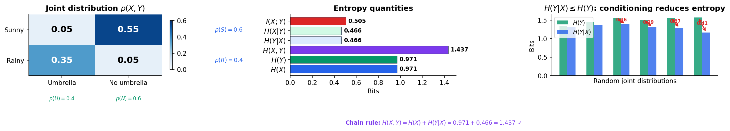
The joint entropy of discrete random variables and is
This is the total uncertainty in the pair — the average number of bits needed to encode both outcomes.
Definition 4 (Conditional Entropy).
The conditional entropy of given is
This is the average remaining uncertainty in after observing .
The chain rule connects these quantities.
Theorem 1 (Chain Rule for Entropy).
More generally, for random variables:
Proof.
The general case follows by induction: , and taking of both sides telescopes.
∎Theorem 2 (Conditioning Reduces Entropy).
with equality if and only if and are independent.
Proof.
We need to show that . This difference is the mutual information (defined in the next section), and its non-negativity follows from the non-negativity of KL divergence:
Equality holds iff for all — independence.
∎In plain language: information can only reduce (or maintain) uncertainty, never increase it. Knowing something extra about the world cannot make you more confused on average.
Mutual Information
Mutual information captures how much knowing one variable tells us about another. It is the fundamental measure of statistical dependence in information theory.
Definition 5 (Mutual Information).
The mutual information between discrete random variables and is
Equivalently:
Mutual information is the KL divergence from the joint distribution to the product of marginals: . It measures how far the joint distribution is from independence.
Proposition 4 (Non-negativity of Mutual Information).
, with equality if and only if and are independent.
Proof.
by the non-negativity of KL divergence (which follows from Jensen’s inequality applied to the convex function ). Equality holds iff for all .
∎Proposition 5 (Symmetry of Mutual Information).
.
Proof.
From the definition: , since joint entropy is symmetric: .
∎This is remarkable: conditioning is asymmetric ( in general), but mutual information is perfectly symmetric. Knowing tells you the same amount about as knowing tells you about .
Proposition 6 (Mutual Information and Independence).
if and only if and are independent.
Proof.
This is a direct consequence of Proposition 4: iff everywhere.
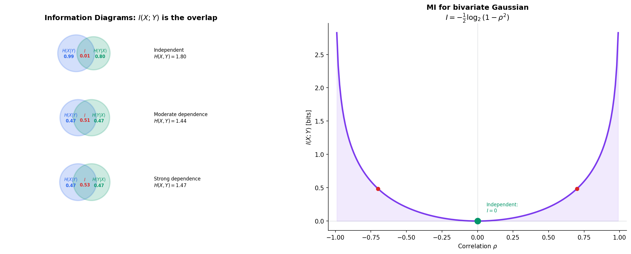
∎The Information Diagram
The relationships between , , , , , and are best visualized as a Venn diagram — the information diagram. Two overlapping circles represent and ; the overlap is ; the left crescent is ; the right crescent is ; and the union is .
Conditional Mutual Information and Chain Rule
Definition 6 (Conditional Mutual Information).
The conditional mutual information of and given is
Theorem 3 (Chain Rule for Mutual Information).
Proof.
Apply the chain rule for entropy to and :
∎
The Data Processing Inequality
The data processing inequality (DPI) is one of the most important results in information theory for machine learning. It formalizes a simple but powerful idea: you cannot create information by processing data.
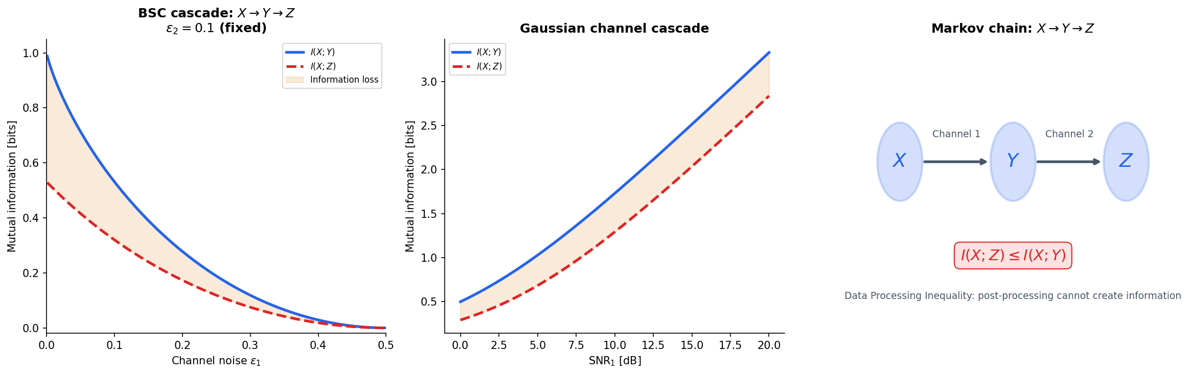
Definition 7 (Markov Chain).
Random variables , , form a Markov chain, written , if is conditionally independent of given :
Equivalently, and are independent given .
Theorem 4 (Data Processing Inequality).
If is a Markov chain, then
Post-processing cannot increase mutual information. Equality holds if and only if is a sufficient statistic of for — that is, .
Proof.
By the chain rule for mutual information:
Since is Markov, , so . Therefore:
Since (non-negativity of conditional MI), we get .
Equality holds iff , meaning provides no additional information about beyond what already captures.
∎The DPI has profound implications for representation learning. Every layer in a neural network processes its input: if we have , then . Information about the input can only decrease through the network. A good representation is one that preserves the relevant information about the target while discarding noise.
Explore the DPI interactively — adjust the channel type and noise level to see how information degrades through processing.
Differential Entropy
What happens when we move from discrete to continuous random variables? The naive approach — replacing sums with integrals — gives differential entropy, but with some important caveats.
Definition 8 (Differential Entropy).
For a continuous random variable with probability density function , the differential entropy is
assuming the integral exists.
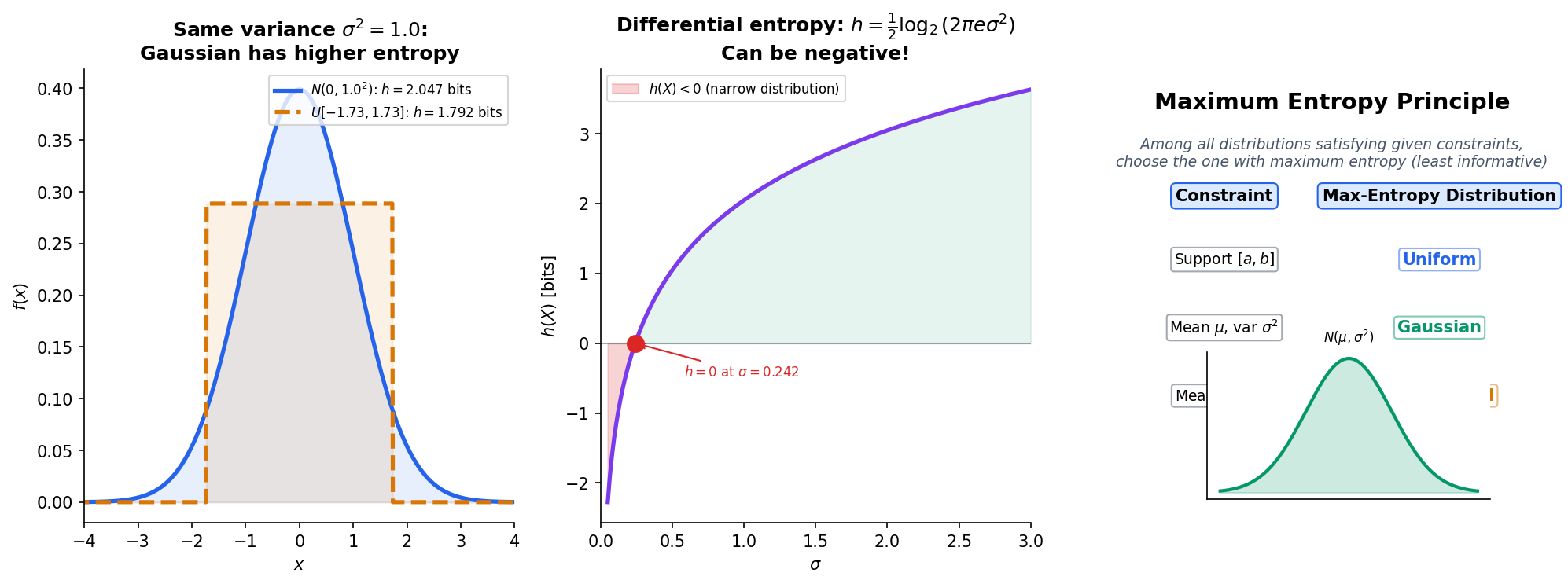
Unlike discrete entropy, differential entropy can be negative — it is not a true measure of “information” in the same absolute sense. However, differences of differential entropies are well-behaved, and mutual information is non-negative even for continuous variables.
Key properties
Translation invariance. for any constant . Shifting a distribution does not change its uncertainty.
Non-invariance under scaling. If for , then . Stretching a distribution increases its entropy; compressing it decreases entropy. This is why differential entropy can be negative — concentrate a distribution enough and .
Maximum Entropy Distribution
Theorem 5 (Gaussian Maximizes Entropy for Fixed Variance).
Among all continuous distributions with mean and variance , the Gaussian uniquely maximizes differential entropy:
with equality if and only if .
Proof.
Let be any density with mean and variance , and let be the Gaussian density . We have:
Now compute . Since :
where we used . Substituting back:
so . Equality holds iff , i.e., .
∎This result explains why Gaussians appear everywhere in statistics and ML: they are the “least informative” distributions for a given variance. When we assume Gaussian noise or Gaussian priors, we are making the maximum-entropy assumption — committing to the distribution that introduces the least extra structure beyond the constraint on variance.

Mutual information for continuous variables
While differential entropy has quirks (negativity, scale-dependence), mutual information remains perfectly well-defined for continuous variables:
This is non-negative and equals zero iff and are independent, just as in the discrete case. The scale-dependent artifacts cancel in the difference.
Source Coding & Compression
Shannon entropy is not just an abstract measure of uncertainty — it has a concrete operational meaning: the entropy of a source is the fundamental limit of lossless data compression. Shannon’s source coding theorem makes this precise.
Prefix codes and Kraft’s inequality
Definition 9 (Prefix Code).
A prefix code (or instantaneous code) assigns a binary codeword to each symbol such that no codeword is a prefix of another. Prefix codes are uniquely decodable without lookahead.
Theorem 6 (Kraft's Inequality).
A prefix code with codeword lengths exists if and only if
Proof.
Necessity. Model the binary code as a complete binary tree of depth . Each codeword of length “claims” a subtree of leaves. Since the prefix property forbids overlap, the total claimed leaves cannot exceed :
Dividing by gives .
Sufficiency. Given lengths satisfying the inequality, assign codewords greedily in order of non-decreasing length, at each step choosing the lexicographically first available codeword. The Kraft inequality guarantees that codewords never run out.
∎Shannon’s source coding theorem
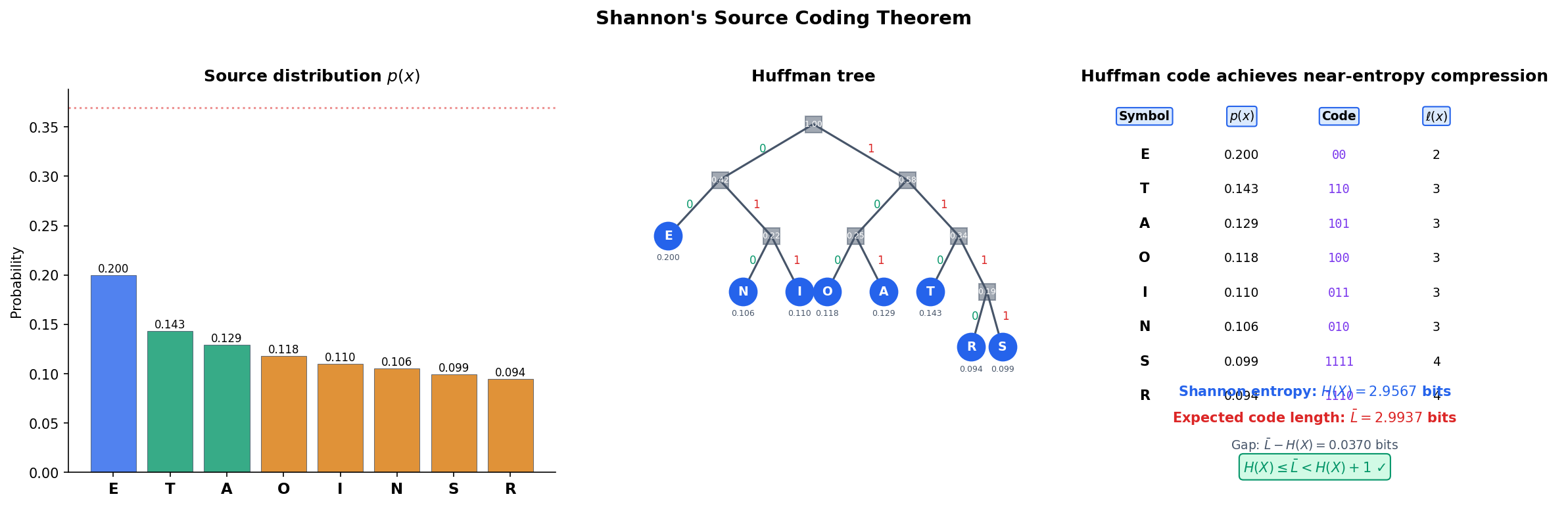
Theorem 7 (Shannon's Source Coding Theorem).
For a discrete random variable with entropy :
- Converse. Any uniquely decodable code must satisfy .
- Achievability. There exists a prefix code with .
In particular, the Huffman code achieves .
Proof.
Converse. By Kraft’s inequality, any code with lengths defines a sub-probability distribution where . Since :
Since and because :
Achievability. Set . Then , so:
These lengths satisfy Kraft’s inequality: .
∎The Huffman algorithm builds an optimal prefix code by iteratively merging the two lowest-probability symbols. Explore the construction below.
| Sym | p(x) | Code | ℓ(x) |
|---|---|---|---|
| A | 0.438 | 0 | 1 |
| B | 0.219 | 10 | 2 |
| C | 0.146 | 110 | 3 |
| D | 0.109 | 1111 | 4 |
| E | 0.088 | 1110 | 4 |

Code blocks: Huffman coding in Python
import heapq

class HuffmanNode:
    def __init__(self, symbol=None, prob=0, left=None, right=None):
        self.symbol = symbol
        self.prob = prob
        self.left = left
        self.right = right

    def __lt__(self, other):
        return self.prob < other.prob

def build_huffman_tree(symbols, probs):
    heap = [HuffmanNode(s, p) for s, p in zip(symbols, probs)]
    heapq.heapify(heap)
    while len(heap) > 1:
        left = heapq.heappop(heap)
        right = heapq.heappop(heap)
        merged = HuffmanNode(prob=left.prob + right.prob, left=left, right=right)
        heapq.heappush(heap, merged)
    return heap[0]

def get_codes(node, prefix='', codes=None):
    if codes is None:
        codes = {}
    if node.symbol is not None:
        codes[node.symbol] = prefix if prefix else '0'
    else:
        if node.left:
            get_codes(node.left, prefix + '0', codes)
        if node.right:
            get_codes(node.right, prefix + '1', codes)
    return codes
Entropy Rate
So far we have studied entropy for single random variables and pairs. For stochastic processes — sequences of random variables — the relevant quantity is the entropy rate: the per-symbol uncertainty in the long run.
Definition 10 (Entropy Rate).
For a stationary stochastic process , the entropy rate is
when the limit exists. Equivalently:
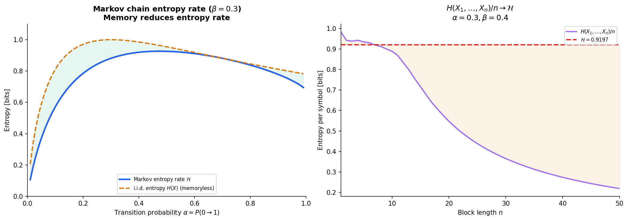
For an i.i.d. process, — each symbol carries its full entropy. But for processes with memory (like Markov chains), the entropy rate is strictly less than because past observations reduce uncertainty about the next symbol.
Proposition 7 (Entropy Rate of a Stationary Markov Chain).
For a stationary Markov chain with transition matrix and stationary distribution , the entropy rate is
where is the entropy of the -th row of the transition matrix.
Proof.
In stationarity, .
By the Markov property, , so the limit defining is reached exactly:
∎
The entropy rate of a Markov chain is a weighted average of the entropies of each row of the transition matrix, weighted by the stationary distribution. States visited more often contribute more to the overall rate.
Computational Notes
Computing entropy in NumPy
import numpy as np

def entropy(probs):
    """Shannon entropy in bits. Convention: 0 log 0 = 0."""
    p = np.asarray(probs, dtype=float)
    p = p[p > 0]  # filter zeros
    return -np.sum(p * np.log2(p))

# Examples
probs_uniform = np.array([0.25, 0.25, 0.25, 0.25])
print(f"Uniform(4): H = {entropy(probs_uniform):.4f} bits")  # 2.0000

probs_peaked = np.array([0.9, 0.05, 0.03, 0.02])
print(f"Peaked:     H = {entropy(probs_peaked):.4f} bits")    # 0.6095
Mutual information from a joint table
def mutual_information(joint):
    """I(X;Y) from a 2D joint probability array."""
    joint = np.asarray(joint, dtype=float)
    p_x = joint.sum(axis=1)
    p_y = joint.sum(axis=0)
    return entropy(p_x) + entropy(p_y) - entropy(joint.ravel())

joint = np.array([[0.3, 0.1],
                   [0.1, 0.5]])
print(f"I(X;Y) = {mutual_information(joint):.4f} bits")
Plug-in vs. k-NN mutual information estimation
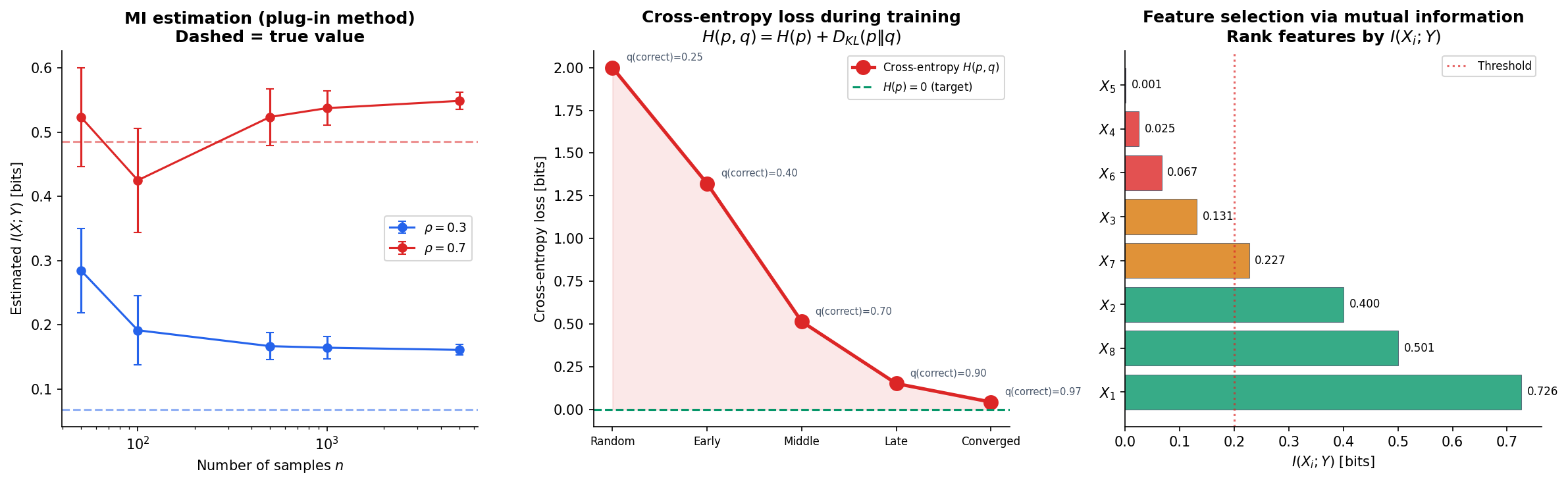
For continuous data, we can estimate MI using either a plug-in estimator (discretize into bins, compute the histogram MI) or the k-nearest-neighbor estimator of Kraskov, Stögbauer & Grassberger (2004), which avoids binning artifacts:
import numpy as np

# Plug-in estimator: discretize and compute
def mi_plugin(x, y, bins='auto'):
    """Plug-in MI estimator via 2D histogram."""
    hist_2d, _, _ = np.histogram2d(x, y, bins=bins)
    hist_2d = hist_2d / hist_2d.sum()  # normalize to joint PMF
    p_x = hist_2d.sum(axis=1)
    p_y = hist_2d.sum(axis=0)
    return entropy(p_x) + entropy(p_y) - entropy(hist_2d.ravel())
The plug-in estimator is biased for small samples (tends to overestimate MI) and sensitive to bin width. The k-NN estimator is consistent and adaptive, making it the preferred method for continuous MI estimation.
Cross-entropy loss and entropy
The cross-entropy loss used in classification is an information-theoretic quantity:
For one-hot labels ( is a point mass), , so . Minimizing cross-entropy loss is equivalent to minimizing the KL divergence from the model’s predicted distribution to the true label distribution.
import torch
import torch.nn.functional as F

# PyTorch cross-entropy loss
logits = torch.tensor([[1.0, 2.0, 0.5, 0.1]])  # raw model outputs
target = torch.tensor([1])                        # true class

loss = F.cross_entropy(logits, target)
print(f"Cross-entropy loss: {loss.item():.4f} nats")

# This equals -log(softmax(logits)[target])
probs = F.softmax(logits, dim=1)
manual_loss = -torch.log(probs[0, target[0]])
print(f"Manual check:       {manual_loss.item():.4f} nats")
Mutual information for feature selection
Rank features by their mutual information with the target variable to identify the most informative features:
This non-parametric criterion captures arbitrary (not just linear) dependencies, making it more powerful than correlation for feature selection in classification tasks.
Connections & Further Reading
Shannon entropy opens the door to a rich web of information-theoretic quantities and their applications across machine learning, statistics, and beyond.
Downstream on this track
- KL Divergence & f-Divergences — the asymmetric divergence generalizes to the broader family of -divergences, each inducing a different geometry on the space of distributions.
- Rate-Distortion Theory — Shannon’s lossy source coding theorem: the minimum rate for encoding a source at distortion level is an optimization over mutual information.
- Minimum Description Length — model selection via code length: the best model minimizes the total description length (model code + data-given-model code), connecting entropy to statistical learning theory.
Cross-track connections
- Measure-Theoretic Probability — entropy is ; differential entropy requires the Lebesgue integral; conditional entropy uses conditional expectation via the Radon–Nikodym theorem.
- Convex Analysis — entropy is concave in ; Jensen’s inequality proves uniform maximality; channel capacity and rate-distortion optimization are convex programs.
- Information Geometry & Fisher Metric — the Fisher metric is the Hessian of KL divergence, which is defined in terms of entropy. The entropy and divergence functions developed here are the starting point for the geometric structure on statistical manifolds.
- Bayesian Nonparametrics — the maximum entropy principle selects the least informative prior consistent with known constraints, connecting entropy to Bayesian inference and the choice of non-informative priors.
- Graph Laplacians & Spectrum — the entropy of a random walk’s stationary distribution measures graph regularity. On a -regular graph, is uniform with maximum entropy . The spectral gap governs the mixing rate — how fast entropy increases toward equilibrium.
Connections
- Entropy is defined as the expectation of the negative log-likelihood: H(X) = E[-log p(X)]. The Lebesgue integral and Radon–Nikodym derivative are essential for differential entropy, and conditional expectation underlies conditional entropy. measure-theoretic-probability
- Entropy is a concave function of the probability distribution — Jensen's inequality gives the maximum entropy property of the uniform distribution. Mutual information optimization (channel capacity, rate-distortion) involves convex programs. convex-analysis
- The Fisher information metric is the Hessian of KL divergence, which is defined in terms of entropy: D_KL(p||q) = H(p,q) - H(p). Shannon entropy is the starting point for the divergence functions that equip statistical manifolds with geometric structure. information-geometry
- Maximum entropy priors (the principle of maximum entropy) select the least informative prior consistent with known constraints, connecting entropy maximization to Bayesian inference. bayesian-nonparametrics
References & Further Reading
- book Elements of Information Theory — Cover & Thomas (2006) The standard reference — Chapters 2-4 cover entropy, mutual information, and source coding
- book Information Theory, Inference, and Learning Algorithms — MacKay (2003) Chapters 2, 4, 5 — information theory with a Bayesian and ML perspective
- paper A Mathematical Theory of Communication — Shannon (1948) The foundational paper — defines entropy, mutual information, and proves the source coding theorem
- book Information Theory and Statistics — Kullback (1968) Classical treatment of the connection between information theory and statistical inference
- book Entropy and Information Theory — Gray (2011) Rigorous measure-theoretic treatment of entropy and entropy rate for stationary processes
- paper Estimating Mutual Information — Kraskov, Stögbauer & Grassberger (2004) k-nearest-neighbor mutual information estimator — the standard non-parametric method