Bayesian Nonparametrics
From the Dirichlet process to Gaussian processes and posterior consistency
Overview & Motivation
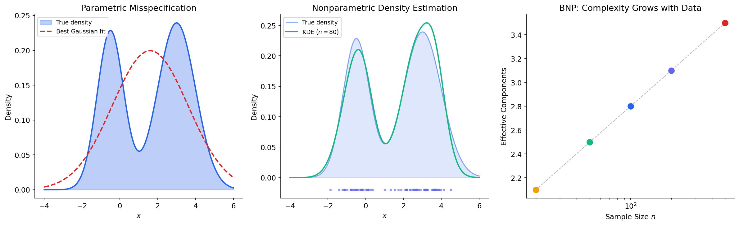
In parametric statistics, we choose a model family — say, Gaussian distributions — and reduce inference to estimating a fixed, finite-dimensional parameter . This works beautifully when the model is well-specified. But what if the true data-generating process is multimodal, heavy-tailed, or otherwise poorly captured by any finite-dimensional family?
The PAC learning framework gave us one answer: control model complexity through the VC dimension or Rademacher complexity, using structural risk minimization (SRM) to balance approximation error and estimation error. Bayesian nonparametrics offers a fundamentally different approach: place a prior directly on an infinite-dimensional parameter space and let the effective complexity of the posterior grow with the data.
The distinction between the two paradigms is worth making precise:
- Parametric models: fix the number of parameters a priori (e.g., fit a mixture of Gaussians).
- Nonparametric models: let the effective number of parameters grow with (e.g., the number of mixture components adapts to the data).
This naming is somewhat misleading — “nonparametric” models have more parameters than parametric ones, not fewer. A better name might be “infinite-parametric,” but the convention is firmly established.
Remark (The Bayesian Resolution of Model Selection).
Recall from the PAC Learning Framework that structural risk minimization balances approximation and estimation error by selecting from a nested sequence of hypothesis classes . Bayesian nonparametrics sidesteps model selection entirely: by placing a prior on the union , the posterior automatically concentrates on the appropriate complexity level. The marginal likelihood provides an automatic “Occam’s razor” — complex models are penalized by the prior unless the data strongly support them.
We’ll develop three canonical nonparametric models in this topic:
- The Dirichlet Process — a prior on probability measures, used for clustering and density estimation.
- The Gaussian Process — a prior on functions, used for regression and classification.
- The Indian Buffet Process — a prior on binary matrices, used for latent feature models.
Each places a prior on an infinite-dimensional object (a measure, a function, a binary matrix with infinitely many columns), yet admits tractable posterior inference through clever constructive representations.
The Dirichlet Distribution
The Dirichlet process is the infinite-dimensional generalization of the Dirichlet distribution, so we begin by reviewing the finite-dimensional case carefully.
Definition 1 (Dirichlet Distribution).
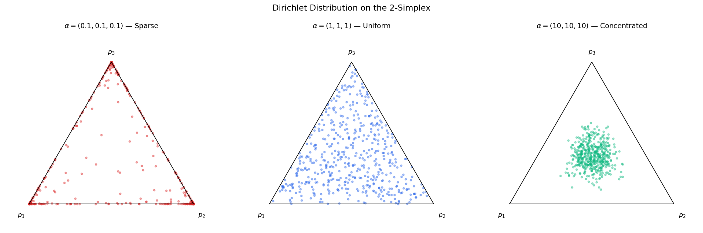
For a positive integer and a parameter vector , the Dirichlet distribution is the probability distribution on the -simplex
with density
where is the gamma function.
The concentration parameter controls how concentrated the distribution is around the base measure :
- When , draws are concentrated near (low variance).
- When , draws are concentrated near the vertices of the simplex (sparse, winner-take-all).
- When and for all , draws are approximately uniform on the simplex.
Proposition 1 (Moments of the Dirichlet).
If with , then:
- ,
- ,
- for .
Proof.
These follow from the integral representation of the beta function. For the mean, note that marginally , so . The variance follows from the Beta variance formula. For the covariance, we use the constraint , which gives . By the symmetry structure of the Dirichlet, all off-diagonal covariances involving have the same sign (negative), and the formula follows from direct computation.
∎Proposition 2 (Dirichlet–Multinomial Conjugacy).
If and , then
Proof.
By Bayes’ theorem, . The multinomial likelihood is , and the Dirichlet prior density is . Multiplying:
which we recognize as .
∎Remark (Aggregation Property).
The Dirichlet distribution satisfies a crucial aggregation property: if and we merge components and into , then the resulting vector follows with the merged parameter. This property is exactly what allows the infinite-dimensional extension — the Dirichlet process — to be self-consistent under arbitrary partitions.
The Dirichlet Process
The Dirichlet process, introduced by Ferguson (1973), is the cornerstone of Bayesian nonparametrics. It is a distribution over probability distributions — a “prior over priors” — that generalizes the Dirichlet distribution to infinite-dimensional spaces.
Definition 2 (Dirichlet Process).
Let be a measurable space, a concentration parameter, and a probability measure on called the base measure. A random probability measure on follows a Dirichlet process, written , if for every finite measurable partition of :
This definition is elegant but requires verification that such an object exists — the condition must be self-consistent across all possible partitions.
Theorem 1 (Existence and Uniqueness of the Dirichlet Process).
For any concentration parameter and base measure on a Polish space , there exists a unique probability measure on the space of probability measures over satisfying the Dirichlet process definition.
Proof.
The key is the Kolmogorov extension theorem. We verify two conditions:
-
Consistency under marginalization. If is a partition and we merge into a single set, the resulting marginal distribution must be . This follows from the aggregation property of the Dirichlet distribution (Remark 2).
-
Consistency under refinement. If we refine into , the joint distribution of must agree with the Dirichlet definition on the finer partition. This follows from the conditional independence structure: , independent of the other components.
With these consistency conditions verified, the Kolmogorov extension theorem guarantees the existence of a unique probability measure on the product -algebra.
∎The two parameters of the DP have clear roles:
- Base measure : the “prior guess” at what looks like. for every measurable — draws from the DP are centered around .
- Concentration parameter : controls how close is to . As , in distribution. As , concentrates on a single atom.
Proposition 3 (Moments of the DP).
If and , then:
- ,
- .
Proof.
These follow directly from the moments of the Beta distribution. For any measurable set , consider the partition . Then , so . The beta distribution gives and .
∎The most surprising — and practically important — property of the Dirichlet process is its almost sure discreteness.
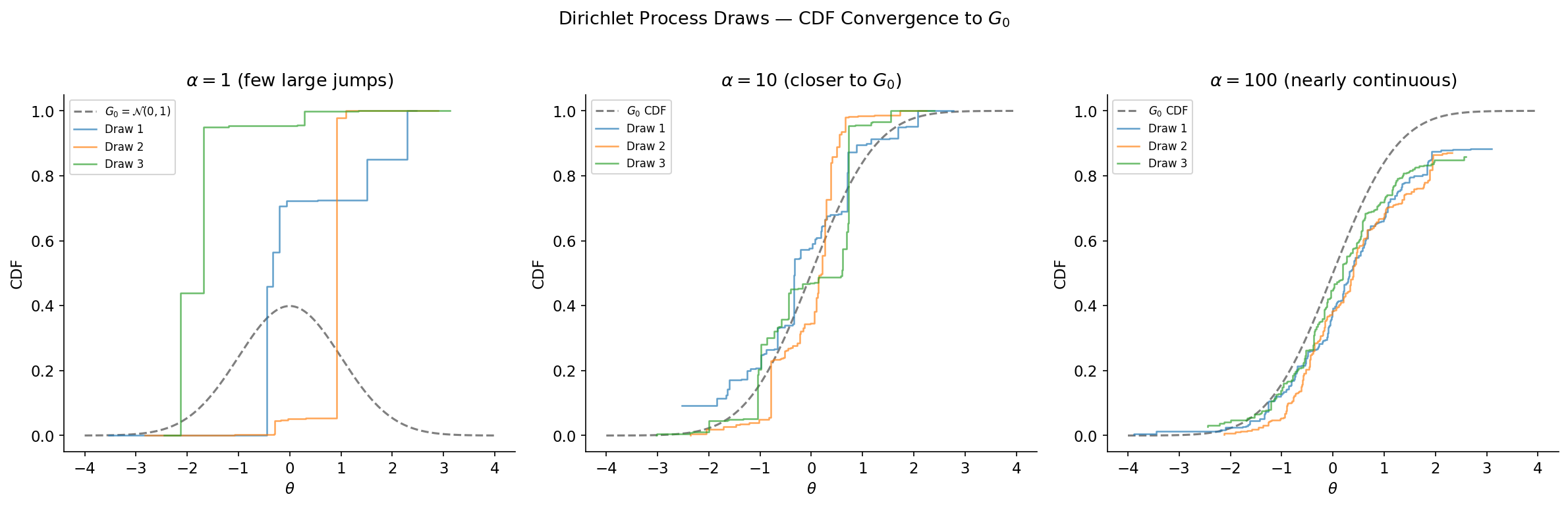
Theorem 2 (Almost Sure Discreteness).
If , then is almost surely a discrete measure, regardless of whether the base measure is continuous or discrete. That is, with probability one,
for some random weights with and random atoms .
Proof.
We prove this via the stick-breaking construction (§4), which provides an explicit representation with and . Since each and , the product almost surely, ensuring almost surely. The atoms are drawn i.i.d. from , so is a countable mixture of point masses.
An alternative argument: for any fixed atom , when is non-atomic. But still has atoms — they arise randomly, not at pre-specified locations. The key insight is that the DP’s finite-dimensional distributions are Dirichlet, and as the partition becomes finer, the mass concentrates on increasingly few partition elements. In the limit, this produces a discrete measure with probability one.
∎Remark (Discreteness Is a Feature, Not a Bug).
The almost sure discreteness of the DP means draws will exhibit ties — multiple observations share the same value. This clustering property is exactly what makes the DP useful for mixture modeling: the number of distinct values (clusters) grows logarithmically with , adapting to the data.
Constructive Representations
Ferguson’s definition (Definition 2) is clean but non-constructive — it tells us the finite-dimensional marginals without directly telling us how to sample from the DP. Three equivalent constructive representations fill this gap, each offering different computational and conceptual advantages.
The Stick-Breaking Construction
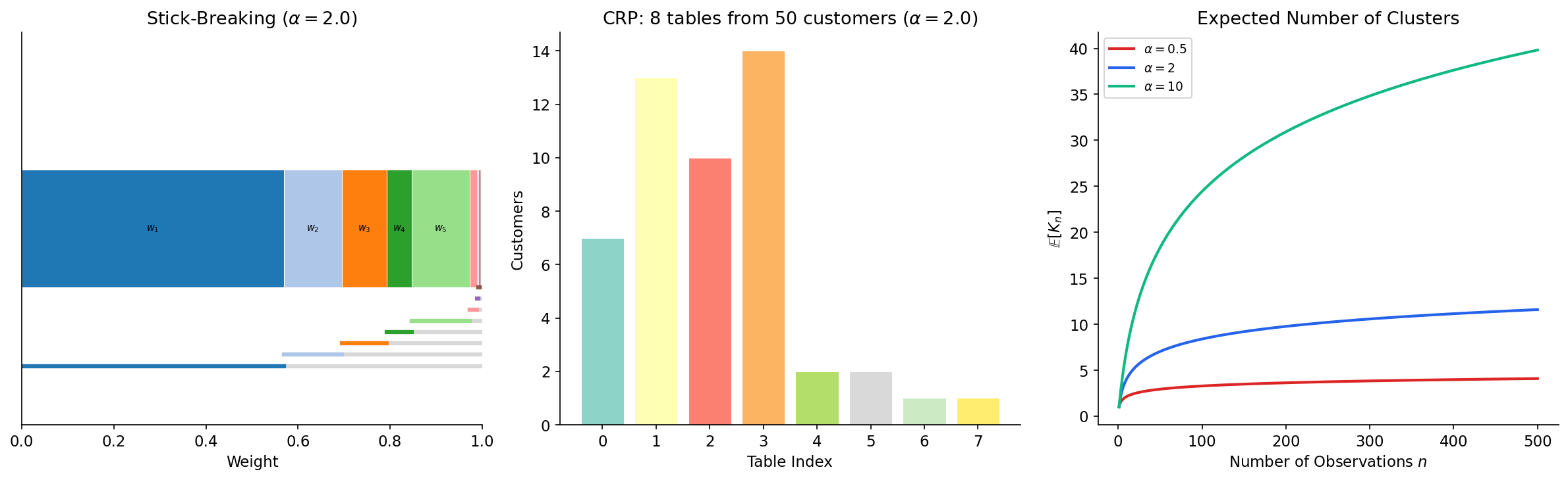
Definition 3 (Stick-Breaking Construction (Sethuraman, 1994)).
Let for and , mutually independent. Define the stick-breaking weights
Then .
The name is vivid: imagine a stick of length 1. Break off a fraction (the first weight ). From the remaining piece of length , break off a fraction (giving ). Continue ad infinitum. The process almost surely exhausts the stick: with probability one.
Theorem 3 (Stick-Breaking Equivalence).
The random measure constructed via stick-breaking is distributed as .
Proof.
We verify the defining property. Let be a finite measurable partition of . Then
We need to show . The proof proceeds by showing that the Laplace transform of matches that of the Dirichlet distribution. Since are i.i.d. and independent of the weights, and the weights have the stick-breaking structure with breaks, this Laplace transform evaluates to the Dirichlet Laplace transform, confirming the DP distribution. The full calculation appears in Sethuraman (1994).
∎
In practice, we truncate the stick-breaking construction at components, which gives an excellent approximation when is large enough:
def stick_breaking_sample(alpha, G0_sampler, K=200):
    """Sample a truncated DP via stick-breaking."""
    V = rng.beta(1, alpha, size=K)
    w = np.zeros(K)
    w[0] = V[0]
    for k in range(1, K):
        w[k] = V[k] * np.prod(1 - V[:k])
    atoms = G0_sampler(K)
    return w, atoms

G0_sampler = lambda K: rng.normal(0, 1, K)The Chinese Restaurant Process
Definition 4 (Chinese Restaurant Process).
Consider a sequence of customers arriving at a restaurant with infinitely many tables. The first customer sits at table 1. Customer sits at:
- an occupied table (with currently customers) with probability ,
- a new table with probability .
When a new table is opened, a dish is drawn for that table. Each customer at table receives the dish associated with their table.
Theorem 4 (CRP–DP Equivalence).
The sequence generated by the Chinese Restaurant Process is exchangeable, and the directing measure (in the sense of de Finetti’s theorem) is .
Proof.
Step 1: Predictive distribution. By the CRP construction, the conditional distribution of given is
This is the Pólya urn predictive rule (Blackwell & MacQueen, 1973).
Step 2: Exchangeability. We verify that is invariant under permutations. The joint probability factors as:
where is the number of distinct values (tables) and is the count at table . This expression depends on only through the partition structure (which values are equal) — not on the ordering. Hence the sequence is exchangeable.
Step 3: De Finetti’s representation. By de Finetti’s theorem, an exchangeable sequence of random variables is a mixture of i.i.d. sequences: for some random . The predictive distribution (Step 1) uniquely identifies through the posterior characterization in §5.
∎The CRP provides an intuitive simulation algorithm:
alpha_crp = 2.0
n_customers = 50
tables = []       # table sizes
assignments = []  # which table each customer sits at

for i in range(n_customers):
    if len(tables) == 0:
        tables.append(1)
        assignments.append(0)
    else:
        probs = np.array(tables + [alpha_crp]) / (i + alpha_crp)
        choice = rng.choice(len(probs), p=probs)
        if choice == len(tables):   # new table
            tables.append(1)
            assignments.append(len(tables) - 1)
        else:                        # existing table
            tables[choice] += 1
            assignments.append(choice)
The Pólya Urn Scheme
Definition 5 (Pólya Urn Scheme (Blackwell & MacQueen, 1973)).
The Pólya urn provides a sequential construction equivalent to the CRP. Start with an urn containing a “paint can” of color with mass . At step :
- Draw a ball from the urn uniformly at random (proportional to mass).
- If the paint can is drawn, generate and add a unit-mass ball of color to the urn.
- If a ball of color is drawn, set and add another unit-mass ball of the same color.
This produces the same predictive rule as the CRP:
Remark (Expected Number of Clusters).
In the CRP, the expected number of distinct tables after customers is
This logarithmic growth is a hallmark of the DP: the number of clusters grows slowly, providing an automatic regularization effect.
Posterior Inference
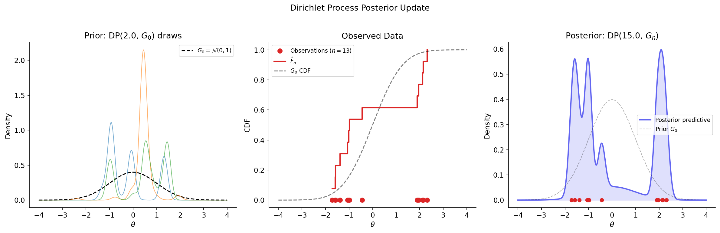
One of the most elegant properties of the Dirichlet process is its conjugacy: the posterior of a DP prior given i.i.d. observations is again a DP, with parameters updated in a natural way.
Theorem 5 (DP Posterior Update).
Let and . Then the posterior distribution of given is
where is the empirical distribution.
Proof.
We verify the defining property of the DP. Let be a finite measurable partition of . Define , so .
Prior. .
Likelihood. Given , the observations are i.i.d. from , so the count vector .
Posterior. By Dirichlet–Multinomial conjugacy (Proposition 2):
We rewrite the updated parameters:
where is the updated base measure. Since this holds for every finite measurable partition, .
∎
Corollary 1 (Posterior Predictive Distribution).
The predictive distribution for given (marginalizing over ) is
Proof.
Integrate against the posterior :
This recovers the Pólya urn predictive rule (Definition 5).
∎Remark (Posterior as Weighted Average).
The posterior base measure is a weighted average of the prior and the empirical distribution . As , the posterior concentrates around — the data overwhelm the prior. As , the posterior stays close to — the prior dominates. This interpolation between prior belief and data evidence is the essence of Bayesian learning.
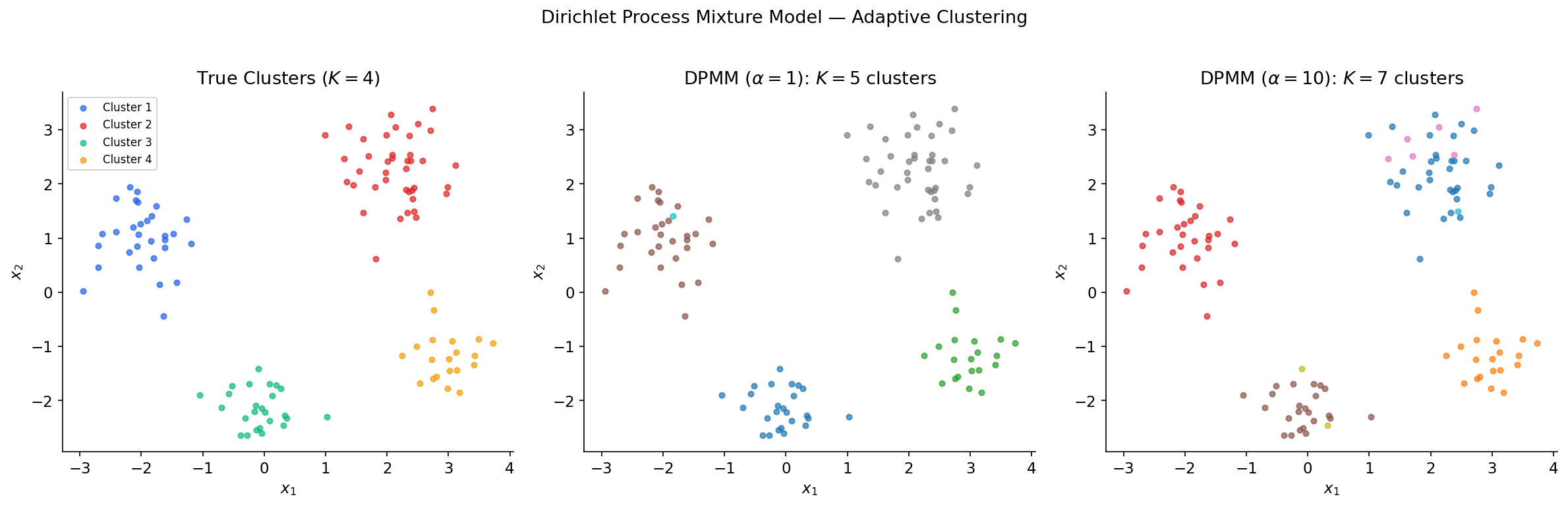
Dirichlet Process Mixture Models
The DP by itself generates discrete distributions, but real data is often continuous. The Dirichlet process mixture model (DPMM) solves this by using the DP as a mixing distribution: each observation is drawn from a kernel (e.g., Gaussian) centered at a DP-sampled atom. This produces a countable mixture with an unknown number of components.
Definition 6 (Dirichlet Process Mixture Model).
A DPMM with concentration parameter , base measure , and kernel is the hierarchical model:
In the Gaussian case with (Normal-Inverse-Wishart) and , this becomes a Gaussian mixture model with a random (potentially infinite) number of components.
The generative process via stick-breaking:
- Draw weights: , set .
- Draw atoms: .
- For each observation : assign to component with , then draw .
Definition 7 (Collapsed DPMM via CRP).
The CRP representation provides an equivalent generative model that integrates out :
- For , assign observation to cluster with probability:
- for existing cluster (where is the count excluding ),
- for a new cluster.
- If assigned to a new cluster, draw .
- Draw .
Gibbs sampling for DPMMs. The collapsed Gibbs sampler (Neal, Algorithm 3) iterates over observations, resampling each cluster assignment from its full conditional:
When the kernel and base measure are conjugate (e.g., Gaussian-NIW), the marginal likelihood and the updated parameter given all observations assigned to cluster have closed-form expressions.
Example 1 (Gaussian DPMM — Univariate).
For with known variance and :
- Marginal likelihood: .
- Posterior for cluster mean: .
def run_dpmm_gibbs(X, alpha, n_iter=50, sigma2=0.5, mu0=0, sigma02=10):
    """Collapsed Gibbs sampler for a univariate Gaussian DPMM."""
    n = len(X)
    z = rng.integers(0, 3, size=n)  # random initial assignments
    for iteration in range(n_iter):
        for i in range(n):
            # Remove observation i from its cluster
            clusters = {}
            for j in range(n):
                if j == i: continue
                clusters.setdefault(z[j], []).append(j)
            probs, cluster_ids = [], []
            for k, members in clusters.items():
                n_k = len(members)
                x_bar = np.mean(X[members])
                precision_post = 1/sigma02 + n_k/sigma2
                mu_post = (mu0/sigma02 + n_k*x_bar/sigma2) / precision_post
                sigma2_pred = sigma2 + 1/precision_post
                log_prob = np.log(n_k) + norm.logpdf(X[i], mu_post, np.sqrt(sigma2_pred))
                probs.append(np.exp(log_prob))
                cluster_ids.append(k)
            # New cluster probability
            log_new = np.log(alpha) + norm.logpdf(X[i], mu0, np.sqrt(sigma2 + sigma02))
            probs.append(np.exp(log_new))
            cluster_ids.append(max(cluster_ids, default=-1) + 1)
            probs = np.array(probs) / sum(probs)
            z[i] = cluster_ids[rng.choice(len(probs), p=probs)]
    return z
Gaussian Processes
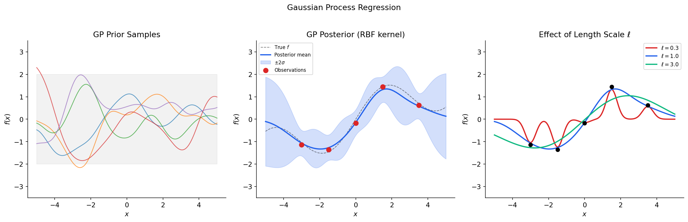
While the Dirichlet process provides a nonparametric prior on probability measures, the Gaussian process provides a nonparametric prior on functions. In the Bayesian nonparametric view, a GP is a prior on an infinite-dimensional function space that admits tractable finite-dimensional marginals.
Definition 8 (Gaussian Process).
A Gaussian process is a collection of random variables , any finite subset of which has a joint Gaussian distribution. A GP is fully specified by its mean function and covariance function (kernel) :
For any finite set of inputs , the function values follow a multivariate Gaussian:
where and .
Definition 9 (Common Kernels).
The choice of kernel encodes prior assumptions about the function:
-
Squared exponential (RBF): — infinitely differentiable functions. Parameters: signal variance , length-scale .
-
Matérn-: — times differentiable. For : .
-
Linear: — equivalent to Bayesian linear regression.
The real power of GPs lies in the closed-form posterior — conditioning on observed data is just Gaussian conditioning.
Theorem 6 (GP Posterior).
Let and observe where . Then the posterior is again a GP with:
where and .
Proof.
Write the joint distribution of the training outputs and the test output :
By the standard formula for Gaussian conditionals ():
Since this holds for any finite set of test points, the posterior is a GP.
∎
In practice, the matrix inverse is computed via the Cholesky decomposition for numerical stability:
def rbf_kernel(X1, X2, length_scale=1.0, signal_var=1.0):
    """Squared exponential (RBF) kernel."""
    sqdist = np.sum(X1**2, 1).reshape(-1, 1) + np.sum(X2**2, 1) - 2 * X1 @ X2.T
    return signal_var * np.exp(-0.5 * sqdist / length_scale**2)

# GP posterior via Cholesky decomposition
K_train = rbf_kernel(X_train, X_train) + sigma_n**2 * np.eye(len(X_train))
K_star = rbf_kernel(X_test, X_train)
K_ss = rbf_kernel(X_test, X_test)

L = np.linalg.cholesky(K_train)                       # O(n^3) factorization
alpha_gp = np.linalg.solve(L.T, np.linalg.solve(L, y_train))  # O(n^2) solve
mu_post = K_star @ alpha_gp                            # posterior mean

v = np.linalg.solve(L, K_star.T)
var_post = np.diag(K_ss) - np.sum(v**2, axis=0)       # posterior variance
std_post = np.sqrt(np.maximum(var_post, 0)) # clamp for numericsRemark (GP–DP Connection).
The Dirichlet process and Gaussian process are complementary nonparametric priors: the DP is a prior on discrete measures (used for clustering and density estimation), while the GP is a prior on continuous functions (used for regression and classification). Both are infinite-dimensional priors with tractable finite-dimensional marginals. The DP’s finite marginals are Dirichlet; the GP’s finite marginals are Gaussian.
The Indian Buffet Process
The Dirichlet process provides a nonparametric prior for clustering (each observation belongs to exactly one cluster). But what if we want each observation to possess multiple latent features? The Indian Buffet Process (IBP), introduced by Griffiths and Ghahramani (2005), provides a nonparametric prior on binary feature matrices with infinitely many columns.
Definition 10 (Indian Buffet Process).
Consider customers sequentially visiting an Indian buffet with infinitely many dishes. Customer 1 tries dishes. Customer (for ):
- tries each previously tasted dish with probability , where is the number of previous customers who tried dish ,
- then tries new dishes that no previous customer has tried.
The result is a random binary matrix , where is the (random, potentially infinite) number of dishes tasted by at least one customer, and if customer tried dish .
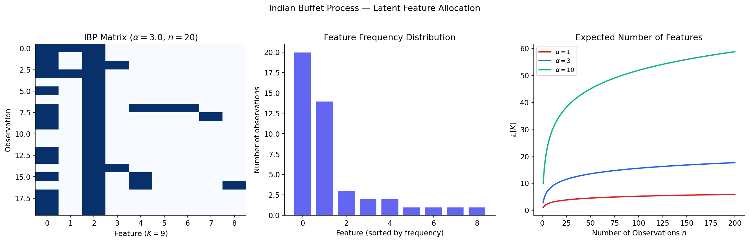
Proposition 4 (Properties of the IBP).
If is generated by the IBP with parameter :
- The expected total number of dishes is , where is the -th harmonic number.
- The expected number of features per customer is .
- The distribution on equivalence classes of binary matrices (up to column permutation) is exchangeable.
Remark (DP vs IBP).
The DP and IBP are complementary priors for different latent structures:
| Property | Dirichlet Process | Indian Buffet Process |
|---|---|---|
| Prior on | Probability measures | Binary matrices |
| Observation model | Each belongs to one cluster | Each has multiple features |
| Analogy | Chinese Restaurant Process | Indian Buffet |
| Underlying process | Beta (stick-breaking) | Beta process |
| Expected components | clusters | features |
The IBP can be derived from a beta process prior, just as the CRP arises from the DP. The beta process is a completely random measure whose atoms have weights in ; each observation independently “selects” each atom with probability equal to its weight, producing the binary matrix .
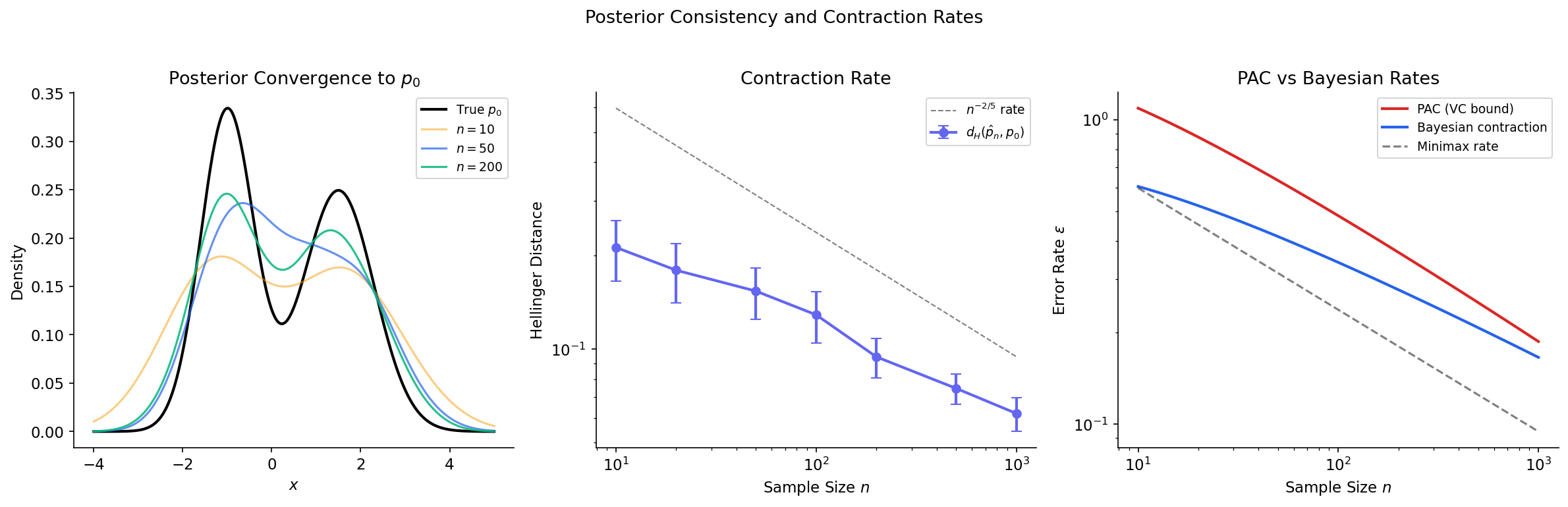
Posterior Consistency and Contraction Rates
The deepest connection between Bayesian nonparametrics and the PAC learning framework lies in the theory of posterior consistency. Just as PAC learning asks “does the learner converge to a good hypothesis as ?”, posterior consistency asks “does the Bayesian posterior converge to the truth?”
Definition 11 (Posterior Consistency).
A Bayesian nonparametric model with prior on a parameter space is posterior consistent at the true parameter if, for every neighborhood of (in an appropriate topology),
Definition 12 (Posterior Contraction Rate).
The posterior contracts at rate around if
for every and some metric on . The rate measures how fast the posterior concentrates.
Schwartz’s Theorem
The classical result on posterior consistency is due to Schwartz (1965), who identified the key condition: the prior must assign positive probability to Kullback-Leibler neighborhoods of the truth.
Theorem 7 (Schwartz's Theorem).
Let be the true data-generating distribution with density , and let be a prior on a space of densities. If is in the Kullback-Leibler support of — that is, for every ,
then the posterior is weakly consistent at : for every weak neighborhood of ,
Proof.
The proof uses three key steps:
- Posterior ratio test. For any measurable set in the complement of , the posterior probability satisfies:
-
Numerator control. By the law of large numbers, for with , the log-likelihood ratio almost surely. The numerator decays exponentially.
-
Denominator control. The KL support condition ensures the denominator does not decay as fast: there exists a “sieve” of densities near that maintain sufficient posterior mass.
Combining, the ratio almost surely.
∎Posterior Contraction Rates
Modern theory (Ghosal, Ghosh & van der Vaart, 2000) goes beyond consistency to rates. The key result establishes that posterior contraction rates are governed by the interplay between prior concentration (how much mass the prior places near the truth) and model complexity (measured by metric entropy).
Theorem 8 (Posterior Contraction Rate (Ghosal, Ghosh & van der Vaart)).
Suppose the following conditions hold for a sequence with :
-
Prior concentration: , where .
-
Sieve complexity: There exist sets (sieves) with and , where is the -covering number.
Then in -probability for sufficiently large .
Remark (Connection to PAC Learning).
The parallel between posterior contraction and PAC learning is striking:
| PAC Learning | Posterior Contraction |
|---|---|
| Sample complexity | Contraction rate |
| VC dimension / Rademacher complexity | Metric entropy |
| Approximation error (bias) | Prior concentration (KL support) |
| Estimation error (variance) | Sieve complexity (covering number) |
| Structural risk minimization | Bayesian model selection (marginal likelihood) |
Both frameworks say: learning succeeds when the model class is rich enough to approximate the truth (low bias) but structured enough to avoid overfitting (controlled complexity). The key difference is the mechanism: PAC bounds are worst-case over distributions, while Bayesian rates depend on the prior and are typically average-case.
Consistency of DP Mixture Models
Proposition 5 (Consistency of DP Gaussian Mixtures).
Let be a distribution with a continuous, bounded density on . A Dirichlet process mixture of Gaussians with base measure and any concentration parameter is posterior consistent at .
Proof.
We verify the KL support condition of Schwartz’s theorem. For any , we need to show .
-
Since Gaussian mixtures are dense in continuous densities (in the sense), for any , there exists a finite Gaussian mixture with .
-
The DP prior assigns positive probability to any finite mixture: the weights can be approximated by stick-breaking weights (each has full support on ), and the atoms can be approximated since is a non-degenerate NIW (with full support on ).
-
Since the KL divergence is continuous in the density (in the topology), a neighborhood of in the prior also satisfies , and this neighborhood has positive prior probability.
Remark (Minimax Rates).
Under regularity conditions (e.g., is -Hölder smooth), DP Gaussian mixture models achieve the near-minimax contraction rate for some . This matches the minimax rate up to a logarithmic factor — the Bayesian nonparametric approach is rate-adaptive, automatically achieving near-optimal rates without needing to know the smoothness in advance.
Connections & Further Reading
Connection Map
| Topic | Domain | Relationship |
|---|---|---|
| PAC Learning Framework | Probability & Statistics | Posterior contraction rates parallel PAC sample complexity; Bayesian model selection provides an alternative to SRM |
| Concentration Inequalities | Probability & Statistics | Posterior contraction proofs use concentration of the log-likelihood ratio; GP concentration bounds use sub-Gaussian tail inequalities |
| Measure-Theoretic Probability | Probability & Statistics | The DP is defined on measure spaces; posterior consistency uses dominated convergence and the law of large numbers |
| Spectral Theorem | Linear Algebra | GP kernel matrices are positive semi-definite; the eigendecomposition of the kernel determines the GP’s RKHS |
| SVD | Linear Algebra | Low-rank GP approximations (Nyström method) use the SVD of the kernel matrix |
| PCA & Low-Rank Approximation | Linear Algebra | Kernel PCA is equivalent to projecting onto the leading eigenfunctions of the GP kernel; functional PCA uses GP priors |
Key Notation Summary
| Symbol | Meaning |
|---|---|
| Dirichlet process with concentration and base measure | |
| Base measure (prior guess for DP draws) | |
| Concentration parameter | |
| Point mass (Dirac delta) at | |
| Dirichlet distribution with parameter vector | |
| Stick-breaking beta variables | |
| Stick-breaking weight | |
| Empirical distribution | |
| Number of distinct clusters after observations | |
| Gaussian process with mean and kernel | |
| GP posterior mean | |
| Kullback-Leibler divergence | |
| -covering number of under metric | |
| Minimax contraction rate for -smooth densities in |
Connections
- Direct prerequisite — posterior contraction rates parallel PAC sample complexity; Bayesian model selection via the marginal likelihood provides an alternative to structural risk minimization. pac-learning
- Foundational — the Dirichlet process is defined on measure spaces; posterior consistency proofs use the law of large numbers, dominated convergence, and Kullback-Leibler divergence. measure-theoretic-probability
- Posterior contraction proofs use concentration of the log-likelihood ratio; Gaussian process concentration bounds use sub-Gaussian tail inequalities. concentration-inequalities
- GP kernel matrices are positive semi-definite; the eigendecomposition of the kernel operator determines the reproducing kernel Hilbert space. spectral-theorem
- Low-rank GP approximations (Nyström method) use the SVD of the kernel matrix. svd
- Kernel PCA is equivalent to projecting onto the leading eigenfunctions of the GP kernel; functional PCA uses GP priors. pca-low-rank
References & Further Reading
- paper A Bayesian Analysis of Some Nonparametric Problems — Ferguson (1973) The foundational paper defining the Dirichlet process
- paper A Constructive Definition of Dirichlet Priors — Sethuraman (1994) The stick-breaking construction
- paper Ferguson Distributions Via Pólya Urn Schemes — Blackwell & MacQueen (1973) The Pólya urn representation and exchangeability
- book Gaussian Processes for Machine Learning — Rasmussen & Williams (2006) Standard reference for GP theory and computation
- book Fundamentals of Nonparametric Bayesian Inference — Ghosal & van der Vaart (2017) Comprehensive treatment of posterior consistency and contraction rates
- paper Infinite Latent Feature Models and the Indian Buffet Process — Griffiths & Ghahramani (2005) Introduction of the IBP
- paper Markov Chain Sampling Methods for Dirichlet Process Mixture Models — Neal (2000) Gibbs sampling algorithms for DPMMs
- paper Convergence rates of posterior distributions — Ghosal, Ghosh & van der Vaart (2000) The general posterior contraction rate theorem
- paper On Bayes procedures — Schwartz (1965) The foundational posterior consistency theorem
- book Bayesian Nonparametrics — Hjort, Holmes, Müller & Walker (2010) Comprehensive survey of BNP methods