The Spectral Theorem
From eigenvalues to geometry — why symmetric matrices are the best-behaved objects in linear algebra
Overview & Motivation
Every machine learning algorithm that touches a covariance matrix, a kernel matrix, a graph Laplacian, or a Hessian is secretly relying on a single theorem: the Spectral Theorem.
The Spectral Theorem says that every real symmetric matrix can be diagonalized by an orthogonal matrix:
where is orthogonal () and is the diagonal matrix of real eigenvalues. This is not just a convenience — it’s a structural guarantee that underpins:
- PCA: the sample covariance matrix is symmetric, so its eigenvectors are orthogonal principal directions.
- Spectral clustering: the graph Laplacian is symmetric positive semidefinite, so its smallest eigenvectors encode cluster structure.
- Optimization: the Hessian is symmetric, and its eigenvalues determine convexity.
- Kernel methods: kernel matrices are symmetric PSD by construction.
- The Sheaf Laplacian: from the Sheaf Theory topic on the Topology & TDA track, is symmetric PSD, and the Spectral Theorem is what makes its eigendecomposition well-defined and interpretable.
This topic develops the Spectral Theorem from first principles, proves it, implements it, and applies it to spectral clustering — building the algebraic foundation that the rest of the Linear Algebra track depends on.
What We Cover
- Eigenvalues & Eigenvectors — characteristic polynomials, eigenspaces, diagonalization.
- Symmetric Matrices & Orthogonality — real eigenvalues, orthogonal eigenvectors, the key lemmas.
- The Spectral Theorem — the full statement and proof, geometric interpretation.
- The Rayleigh Quotient — variational characterization of eigenvalues, the Courant–Fischer min-max theorem.
- Quadratic Forms & Definiteness — positive definiteness, Sylvester’s criterion.
- Spectral Decomposition in Practice — power iteration, the QR algorithm.
- Application: Spectral Clustering — from similarity graph to clusters via the graph Laplacian’s eigenvectors.
- Application: PCA Preview — the Spectral Theorem applied to the covariance matrix.
Eigenvalues & Eigenvectors
The Eigenvalue Problem
Given a square matrix , a scalar is an eigenvalue of if there exists a nonzero vector such that:
The vector is the eigenvector corresponding to . Geometrically, acts on by simply scaling it — is a direction that preserves.
Definition 1 (Eigenvalue and Eigenvector).
Let . A scalar is an eigenvalue of if there exists a nonzero vector such that . The vector is an eigenvector corresponding to .
The Characteristic Polynomial
Rearranging gives , which has a nonzero solution if and only if:
Definition 2 (Characteristic Polynomial).
The characteristic polynomial of is . For an matrix, it has degree , so by the Fundamental Theorem of Algebra there are exactly eigenvalues (counted with algebraic multiplicity) in .
Eigenspaces and Multiplicity
Definition 3 (Eigenspace, Algebraic and Geometric Multiplicity).
The eigenspace for eigenvalue is — the set of all eigenvectors for plus the zero vector. The algebraic multiplicity is the multiplicity of as a root of . The geometric multiplicity is the dimension of the eigenspace. Always .
When for some , the matrix is defective and cannot be diagonalized. A central result of this topic is that symmetric matrices are never defective.
Symmetric Matrices & Orthogonality
A matrix is symmetric if , meaning for all . Symmetric matrices appear everywhere in ML:
- Covariance matrices:
- Graph Laplacians:
- Hessians: (by equality of mixed partials)
- Kernel matrices:
- Gram matrices:
The three lemmas below are the building blocks of the Spectral Theorem.
Real Eigenvalues
Lemma 1 (Real Eigenvalues of Symmetric Matrices).
Every eigenvalue of a real symmetric matrix is real.
Proof.
Let and suppose with , where and . Consider:
Now take the conjugate transpose of . Since is real symmetric:
But , giving us . Since , we conclude , i.e., .
∎Orthogonal Eigenvectors
Lemma 2 (Orthogonal Eigenvectors for Distinct Eigenvalues).
Eigenvectors of a real symmetric matrix corresponding to distinct eigenvalues are orthogonal.
Proof.
Let and with . Then:
So . Since , we must have .
∎Invariant Complements
Lemma 3 (Invariant Complements).
If is real symmetric and is an -invariant subspace (meaning for all ), then is also -invariant.
Proof.
Let and . Then since and . So for all , meaning .
∎This lemma is the engine of the inductive proof: once we find one eigenvector, we can restrict to its orthogonal complement and repeat.
The Spectral Theorem
Statement
Theorem 1 (Spectral Theorem for Real Symmetric Matrices).
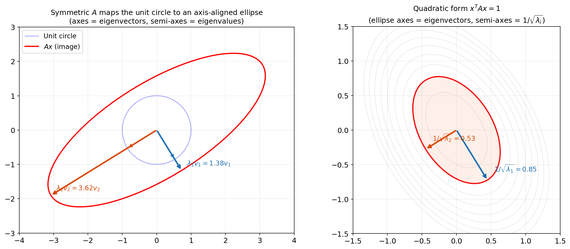
Let be symmetric. Then there exists an orthogonal matrix (with ) and a diagonal matrix with such that:
where are the columns of — an orthonormal basis of eigenvectors.
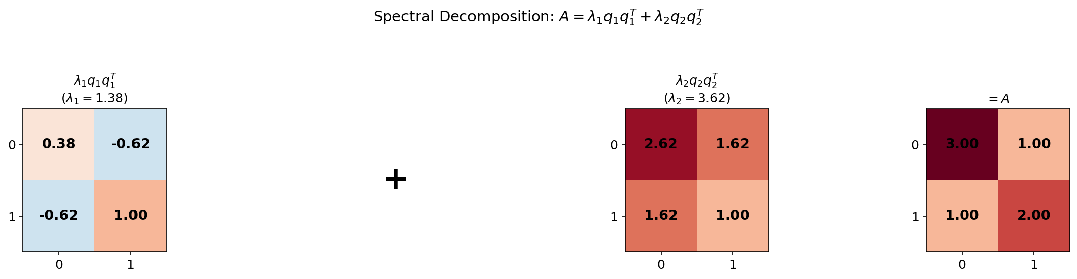
The second form — the spectral decomposition — writes as a sum of rank-1 projection matrices , each scaled by its eigenvalue. This is the form that directly gives PCA its interpretation.
Proof
Proof.
By induction on .
Base case (). Every matrix is trivially diagonalized: , .
Inductive step. Assume the theorem holds for all symmetric matrices of size . Let be and symmetric.
Step 1. has at least one eigenvalue (by Lemma 1, all eigenvalues are real; and the characteristic polynomial has degree , so it has at least one root). Let be a corresponding unit eigenvector: , .
Step 2. Let . By Lemma 3, is -invariant. Choose any orthonormal basis for and let be the matrix whose columns are this basis.
Step 3. Define . Then is symmetric: .
Step 4. By the inductive hypothesis, for some orthogonal and diagonal .
Step 5. Set . Then is orthogonal, and:
So where .
∎Geometric Interpretation
The Spectral Theorem says that every symmetric linear transformation is, in the right coordinate system, just a stretch along orthogonal axes. The eigenvectors define the axes, and the eigenvalues define the stretch factors.
This is why:
- Covariance matrices define ellipsoidal level sets (axes = principal components).
- Graph Laplacians have smooth eigenvectors that partition the graph.
- Hessians at critical points tell you whether you’re at a min, max, or saddle — by the signs of the eigenvalues along orthogonal curvature directions.
Try it yourself — drag the sliders to change the matrix entries and watch the eigenvectors and ellipse update in real time:
The Hermitian Extension
The Spectral Theorem extends to Hermitian (complex self-adjoint) matrices. A matrix with has:
where is unitary () and is real diagonal. The proof is identical, replacing transposes with conjugate transposes. Every real symmetric matrix is Hermitian, so the real version is a special case.
Numerical Verification
We can verify the Spectral Theorem in code. Here np.linalg.eigh is the dedicated function for symmetric/Hermitian matrices — it guarantees real eigenvalues and orthonormal eigenvectors:
import numpy as np

A = np.array([
    [5, 2, 0, 1],
    [2, 4, 1, 0],
    [0, 1, 3, 2],
    [1, 0, 2, 6]
], dtype=float)

# eigh is specifically for symmetric matrices
eigenvalues, Q = np.linalg.eigh(A)
Lambda = np.diag(eigenvalues)

# Verify A = Q Lambda Q^T
print(f"||A - Q Lambda Q^T||_F = {np.linalg.norm(A - Q @ Lambda @ Q.T):.2e}")
# Output: 1.01e-14

# Spectral decomposition: A = sum lambda_i q_i q_i^T
A_spectral = sum(eigenvalues[i] * np.outer(Q[:, i], Q[:, i]) for i in range(A.shape[0]))
print(f"||A - sum lambda_i q_i q_i^T||_F = {np.linalg.norm(A - A_spectral):.2e}")
# Output: 1.03e-14
The Rayleigh Quotient
Definition
Definition 4 (Rayleigh Quotient).
The Rayleigh quotient of a symmetric matrix at a nonzero vector is:
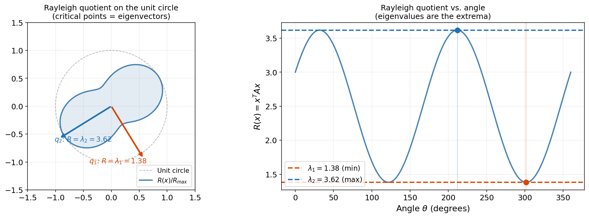
On the unit sphere , this simplifies to . Its critical points are the eigenvectors, and its critical values are the eigenvalues.
The Rayleigh quotient is the bridge between eigenvalues and optimization. Its value tells you “how much stretches in the direction ” — and the eigenvectors are the directions where this stretch is extremal.
Extremal Characterization
Proposition 1 (Extremal Characterization of Eigenvalues).
For a symmetric matrix with eigenvalues :
The minimum is attained at (the eigenvector for ) and the maximum at .
Proof.
Write with (since is an ONB). Then:
Equality holds when and all other , i.e., . The maximum case is analogous.
∎The interactive visualization below shows the Rayleigh quotient as traces the unit circle. The polar plot reveals how the quadratic form bulges in the eigenvector directions, and the Cartesian plot shows the extrema at and :
A = [[3.0, 1.0], [1.0, 2.0]] — 1.38 ≤ R(x) ≤ 3.62
The Courant–Fischer Min-Max Theorem
Theorem 2 (Courant–Fischer Min-Max Theorem).
For a symmetric matrix with eigenvalues :
This characterizes the -th eigenvalue as a min-max over subspaces. It is the theoretical foundation of PCA: the -th principal component maximizes variance subject to orthogonality with the first components — exactly the Courant–Fischer characterization applied to the covariance matrix.
Quadratic Forms & Definiteness
Quadratic Forms
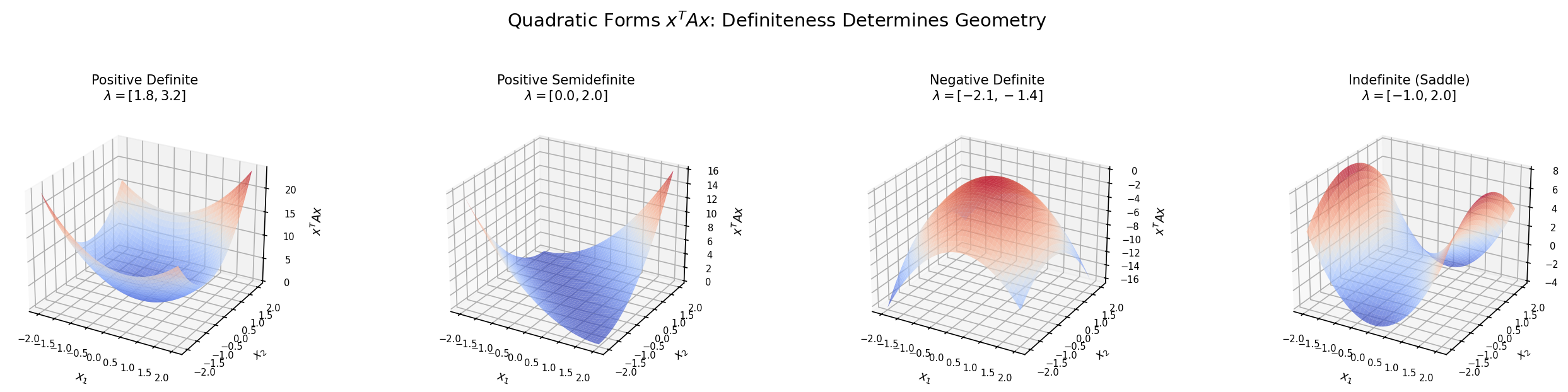
Definition 5 (Quadratic Form and Definiteness).
A quadratic form on is a function for a symmetric matrix . The definiteness of is determined by the signs of its eigenvalues:
| Condition | Name | Eigenvalues | Geometry |
|---|---|---|---|
| for all | Positive definite (PD) | All | Bowl |
| for all | Positive semidefinite (PSD) | All | Bowl with flat directions |
| for all | Negative definite (ND) | All | Inverted bowl |
| for all | Negative semidefinite (NSD) | All | Inverted bowl with flat |
| Signs mixed | Indefinite | Some , some | Saddle |
Why definiteness matters for ML: A covariance matrix is always PSD (). A graph Laplacian is PSD. A kernel matrix is PSD by Mercer’s theorem. The Hessian at a local minimum is PSD.
Sylvester’s Criterion
Theorem 3 (Sylvester's Criterion).
A symmetric matrix is positive definite if and only if all its leading principal minors are positive:
This gives a determinant-based test that avoids computing eigenvalues — useful for theoretical arguments and small matrices.
Spectral Decomposition in Practice
eig vs. eigh
Two functions for eigendecomposition:
| Function | For | Algorithm | Guarantees |
|---|---|---|---|
np.linalg.eig(A) | General square matrices | QR iteration (LAPACK dgeev) | May return complex values |
np.linalg.eigh(A) | Symmetric/Hermitian | Divide-and-conquer (LAPACK dsyevd) | Real eigenvalues; orthonormal eigenvectors |
Always use eigh for symmetric matrices. It is faster ( vs. ), more numerically stable, and guarantees the Spectral Theorem’s output format.
Power Iteration
The power method is the simplest eigenvalue algorithm: repeatedly multiply by and normalize. This converges to the dominant eigenvector at a rate proportional to — the ratio of the two largest eigenvalues.
def power_iteration(A, max_iter=100, tol=1e-10):
    """Power iteration for the dominant eigenpair of a symmetric matrix."""
    n = A.shape[0]
    x = np.random.randn(n)
    x = x / np.linalg.norm(x)

    lam = 0.0
    for _ in range(max_iter):
        y = A @ x
        lam_new = x @ y  # Rayleigh quotient
        x_new = y / np.linalg.norm(y)

        if abs(lam_new - lam) < tol:
            lam = lam_new
            x = x_new
            break

        lam = lam_new
        x = x_new

    return lam, x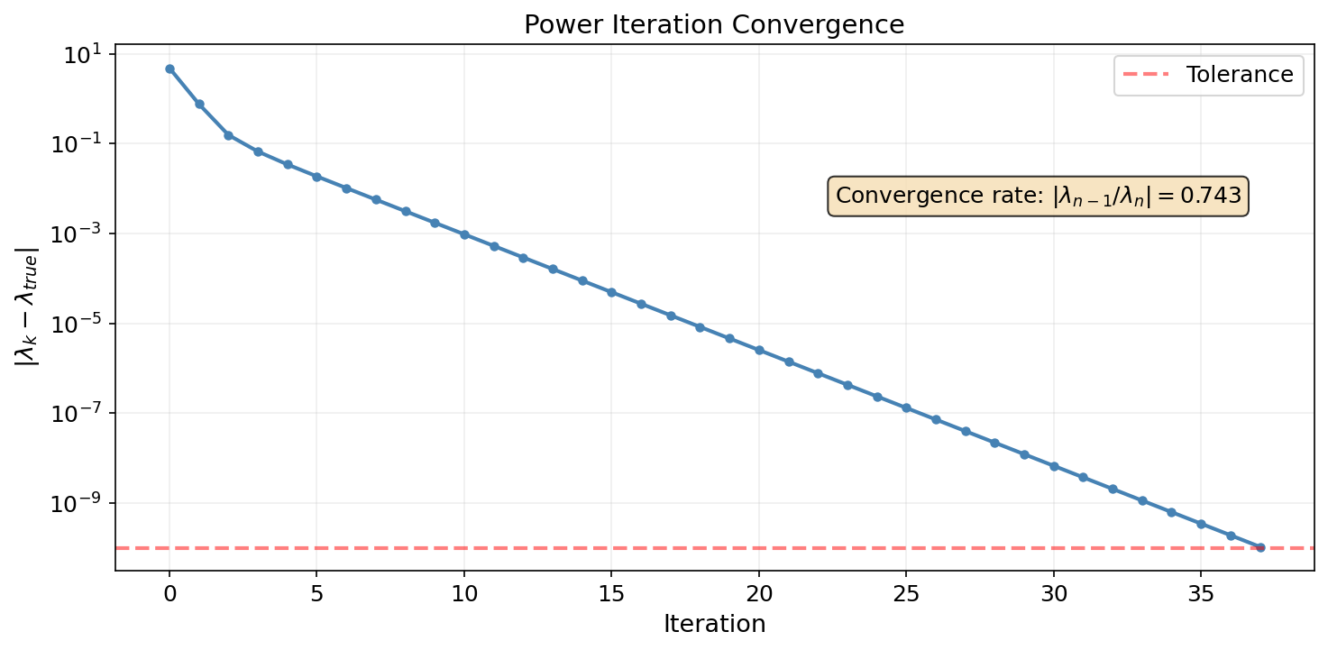
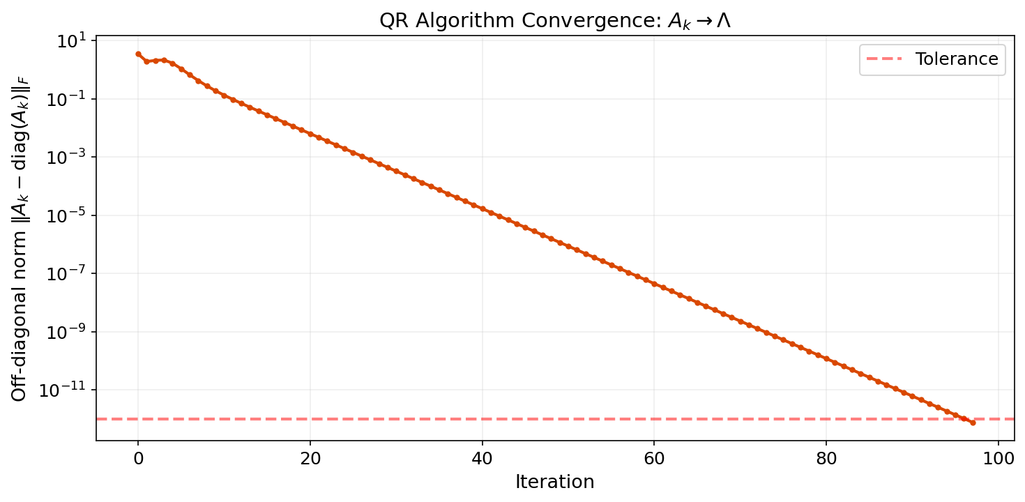
The QR Algorithm
The industry-standard eigenvalue algorithm is the QR algorithm: repeatedly factor and form . This is a similarity transformation (), so eigenvalues are preserved — but converges to diagonal form.
def qr_algorithm(A, max_iter=200, tol=1e-12):
    """Basic QR algorithm (without shifts) for a symmetric matrix."""
    Ak = A.copy()

    for k in range(max_iter):
        Q, R = np.linalg.qr(Ak)
        Ak = R @ Q  # similarity transform: same eigenvalues

        off_diag = np.linalg.norm(Ak - np.diag(np.diag(Ak)))
        if off_diag < tol:
            break

    return np.sort(np.diag(Ak))
With shifts, deflation, and Householder reductions, the production QR algorithm achieves complexity. The basic version above converges at a rate determined by the eigenvalue ratios — similar to power iteration, but for all eigenvalues simultaneously.
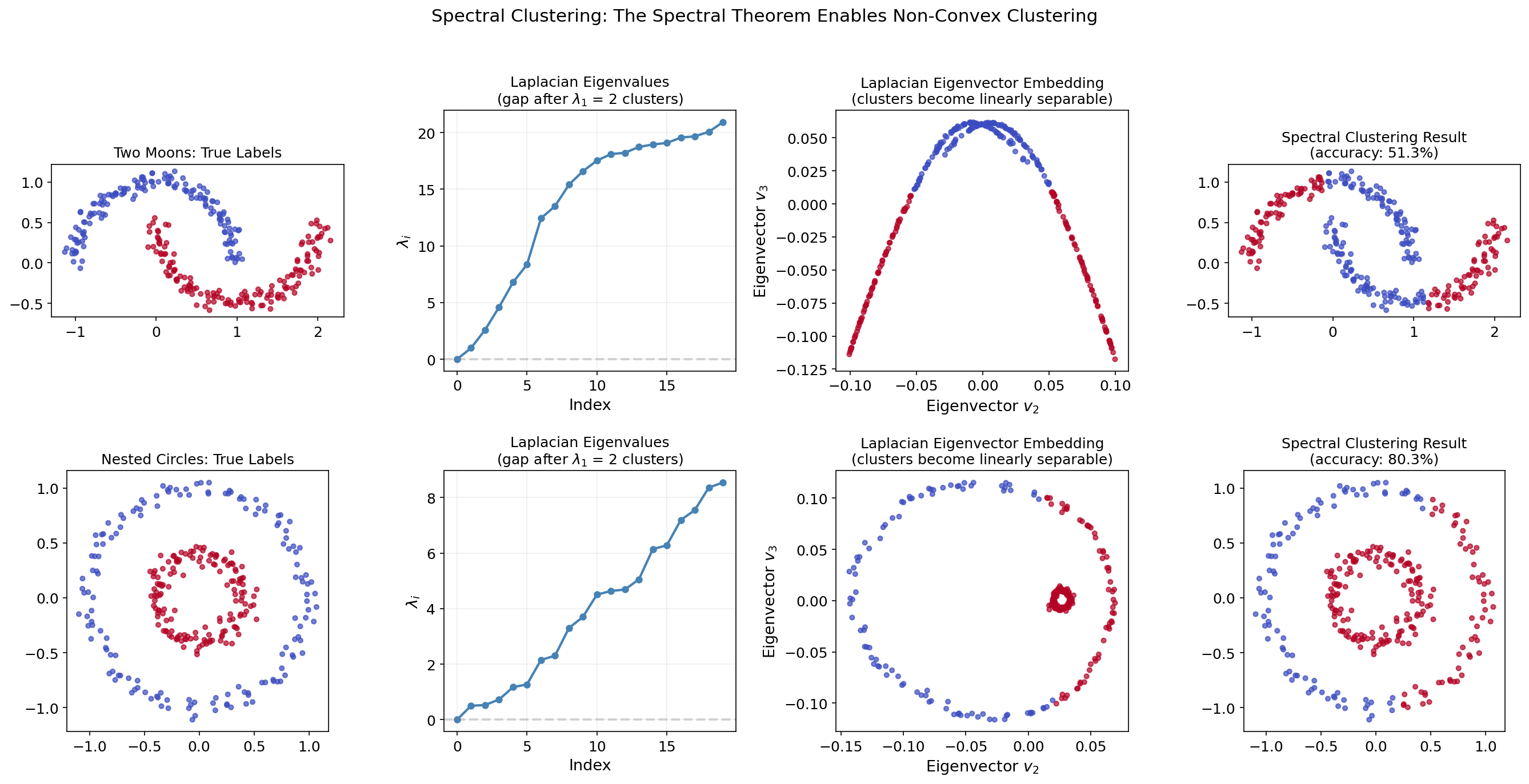
Application: Spectral Clustering
Spectral clustering is the flagship application of the Spectral Theorem in unsupervised learning. The idea: transform data using the eigenvectors of a graph Laplacian, then cluster in the transformed space.
Why Spectral Clustering?
Standard k-means clustering fails on non-convex clusters (e.g., nested circles or interleaving moons). Spectral clustering handles these by:
- Building a similarity graph from the data.
- Computing the graph Laplacian (a symmetric PSD matrix).
- Using the Spectral Theorem to find its smallest eigenvectors.
- Clustering in the eigenvector embedding space.
The Graph Laplacian
Given a weighted adjacency matrix (with for Gaussian similarity), the unnormalized graph Laplacian is:
where with .
Key properties (all from the Spectral Theorem):
- is symmetric (since is symmetric).
- is PSD: .
- The number of zero eigenvalues of equals the number of connected components.
- The eigenvectors for the smallest eigenvalues encode cluster structure.
The Algorithm
- Build the similarity matrix (e.g., Gaussian kernel with bandwidth ).
- Compute .
- Compute the smallest eigenvectors of : .
- Form the matrix with columns .
- Run k-means on the rows of .
Interactive Demo
Step through the spectral clustering pipeline on a two-moons dataset. Watch how the Laplacian’s eigenvectors transform a non-convex clustering problem into a linearly separable one:
Implementation
from scipy.spatial.distance import pdist, squareform
from sklearn.cluster import KMeans

def spectral_clustering(X, k, sigma=1.0):
    """Spectral clustering using the unnormalized graph Laplacian."""
    # Step 1: Similarity matrix (Gaussian kernel)
    dists = squareform(pdist(X, 'sqeuclidean'))
    W = np.exp(-dists / (2 * sigma**2))
    np.fill_diagonal(W, 0)

    # Step 2: Graph Laplacian
    D = np.diag(W.sum(axis=1))
    L = D - W

    # Step 3: Smallest k eigenvectors (skip constant eigenvector)
    eigenvalues, eigenvectors = np.linalg.eigh(L)
    U = eigenvectors[:, 1:k+1]

    # Step 4: Normalize rows
    row_norms = np.linalg.norm(U, axis=1, keepdims=True)
    U_norm = U / np.where(row_norms < 1e-10, 1, row_norms)

    # Step 5: K-means on the embedding
    labels = KMeans(n_clusters=k, random_state=42, n_init=10).fit_predict(U_norm)
    return labels
The graph Laplacian is symmetric PSD, so the Spectral Theorem guarantees real eigenvalues, orthogonal eigenvectors, and a well-defined spectral gap — exactly the properties that make spectral clustering work.
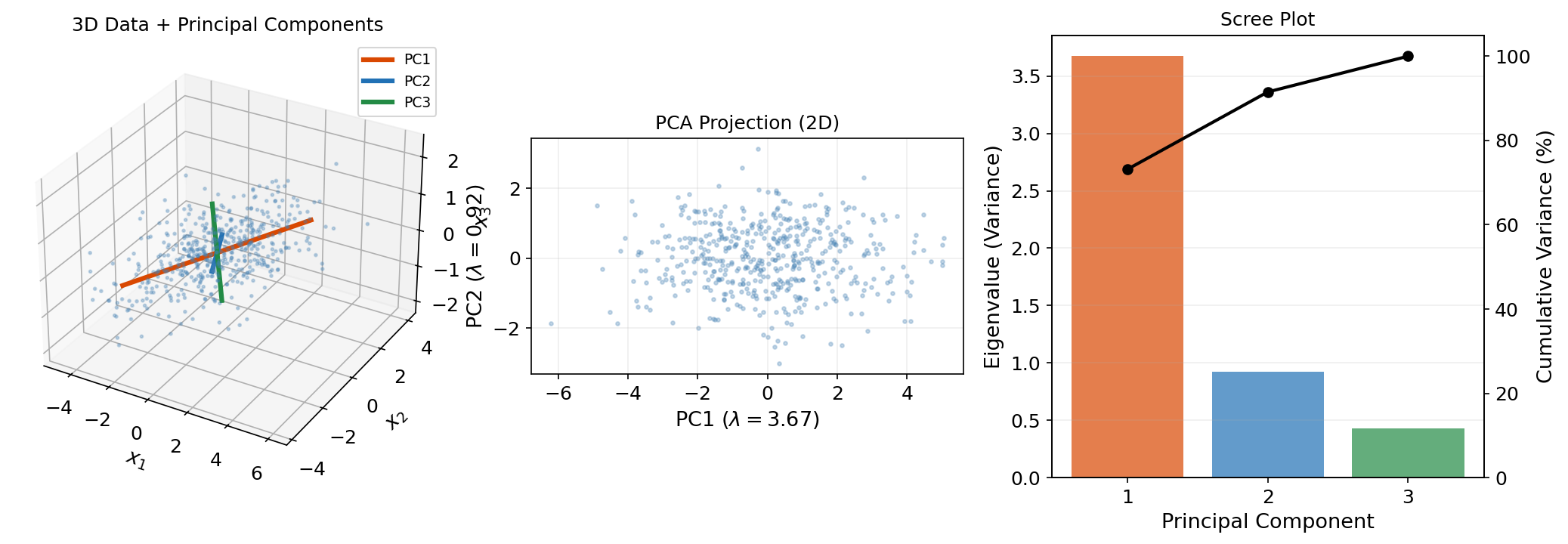
Application: PCA Preview
Principal Component Analysis is the Spectral Theorem applied to the sample covariance matrix. The full development lives on the PCA & Low-Rank Approximation topic page — here we establish the connection.
The Covariance Matrix Is Symmetric PSD
Given centered data (rows = observations, columns = features), the sample covariance matrix is:
This is symmetric () and PSD ().
PCA as the Spectral Theorem
By the Spectral Theorem, with orthogonal and diagonal (non-negative). The columns of are the principal components — orthogonal directions of maximum variance. The eigenvalues are the variances along these directions.
# PCA via eigendecomposition of the covariance matrix
X_centered = X - X.mean(axis=0)
Sigma_hat = (X_centered.T @ X_centered) / (n - 1)

eigenvalues, Q = np.linalg.eigh(Sigma_hat)
# eigh returns ascending order; PCA wants descending
idx = np.argsort(eigenvalues)[::-1]
eigenvalues, Q = eigenvalues[idx], Q[:, idx]

# Project onto first k principal components
X_pca = X_centered @ Q[:, :k]
The Courant–Fischer theorem (Theorem 2) guarantees this is the optimal rank- variance-preserving projection.
The SVD Connection
PCA is also connected to the Singular Value Decomposition (the next topic in this track). If is the SVD, then , so the right singular vectors of are the eigenvectors of . The SVD generalizes the Spectral Theorem to rectangular matrices — the subject of the next topic.
Connections & Further Reading
The Spectral Theorem is the algebraic foundation that supports the entire Linear Algebra track and connects back to the Topology & TDA track.
| Topic | Connection |
|---|---|
| Singular Value Decomposition | The SVD generalizes the Spectral Theorem to rectangular matrices. For symmetric , the SVD reduces to the spectral decomposition. |
| PCA & Low-Rank Approximation | PCA is the Spectral Theorem applied to . The Eckart–Young theorem follows from the spectral decomposition. |
| Tensor Decompositions | The CP decomposition generalizes eigendecomposition to tensors. Symmetric tensor decomposition is the higher-order analog of the Spectral Theorem. |
| Sheaf Theory | The Sheaf Laplacian is symmetric PSD. The Spectral Theorem guarantees its eigendecomposition. is read from the zero eigenvalues. |
| Convex Analysis | The second-order convexity condition: is verified through the eigendecomposition guaranteed by the Spectral Theorem. The PSD cone is a fundamental convex set. |
| Graph Laplacians & Spectrum | The graph Laplacian is a real symmetric matrix. The Spectral Theorem guarantees its complete orthonormal eigenbasis — the foundation of spectral graph theory, spectral clustering, and graph neural networks. |
| Categories & Functors | The category Vec of finite-dimensional vector spaces and linear maps is the primary running example in category theory. The Spectral Theorem guarantees that symmetric endomorphisms in Vec have complete eigenbases. illustrates the Hom functor concretely. |
The Linear Algebra Track
The Spectral Theorem is the root of the track: everything that follows either extends it (SVD → rectangular matrices, tensors → higher order) or applies it (PCA → optimal projection).
Spectral Theorem (this topic)
    ├── Singular Value Decomposition
    │       └── PCA & Low-Rank Approximation
    └── Tensor Decompositions
Connections
- the SVD generalizes the Spectral Theorem to rectangular matrices; for symmetric A, the SVD and spectral decomposition coincide svd
- PCA is the Spectral Theorem applied to the sample covariance matrix pca-low-rank
- symmetric tensor decomposition is the higher-order analog of the Spectral Theorem tensor-decompositions
- the Sheaf Laplacian is symmetric PSD; the Spectral Theorem guarantees its eigendecomposition sheaf-theory
- The second-order convexity condition requires the Hessian to be PSD — the Spectral Theorem provides the eigendecomposition that verifies this. convex-analysis
- The tangent space at each point of a smooth manifold is a real vector space. A Riemannian metric makes curvature-related operators (such as the shape operator or curvature operator) symmetric, and the Spectral Theorem diagonalizes these maps so that their eigenvalues encode geometric invariants like principal or sectional curvatures. smooth-manifolds
References & Further Reading
- book Introduction to Linear Algebra — Strang (2016) Primary pedagogical reference
- book Matrix Analysis — Horn & Johnson (2013) Rigorous proofs and spectral theory
- book Numerical Linear Algebra — Trefethen & Bau (1997) QR algorithm and numerical methods
- book Linear Algebra Done Right — Axler (2024) Clean theoretical development
- paper A tutorial on spectral clustering — von Luxburg (2007) Spectral clustering application
- paper Normalized cuts and image segmentation — Shi & Malik (2000) Normalized graph Laplacian for clustering
- paper On spectral clustering: Analysis and an algorithm — Ng, Jordan & Weiss (2001) Normalized spectral clustering algorithm
- paper Toward a spectral theory of cellular sheaves — Hansen & Ghrist (2019) Sheaf Laplacian spectral theory — cross-track connection