Tensor Decompositions
From multi-way arrays to modern factorization — generalizing the SVD and PCA to higher-order data
Overview & Motivation
Matrices are two-way arrays: rows and columns. But many datasets are naturally multi-way. A color image is a 3-way array (height × width × RGB channels). A video is 4-way (height × width × channels × time). A recommender system logs users × items × context × time. EEG data has channels × time × trials. In each case, flattening the data into a matrix and applying the SVD or PCA destroys multi-way structure that the decomposition should preserve.
Tensor decompositions generalize matrix factorizations to multi-way arrays — or tensors — preserving the multi-way structure while achieving compression, denoising, and interpretable factor extraction. The two classical decompositions are:
- CP (CANDECOMP/PARAFAC): Decomposes a tensor into a sum of rank-1 terms (outer products of vectors). This is the natural generalization of the matrix rank-1 decomposition from the SVD topic.
- Tucker decomposition: Decomposes a tensor into a core tensor multiplied by a factor matrix along each mode. This generalizes PCA: each factor matrix captures the principal subspace along one mode, and the core tensor captures multi-mode interactions.
Beyond these classical methods, we develop three modern decompositions:
- HOSVD (Higher-Order SVD): A specific Tucker decomposition computed by applying the matrix SVD along each mode. It provides the tensor analog of the Spectral Theorem’s eigendecomposition.
- Tensor Train (TT): A chain-structured decomposition that avoids the exponential blow-up of Tucker, scaling linearly in the number of modes. Also known as Matrix Product States (MPS) in quantum physics.
- t-SVD (tensor SVD via the Fourier domain): An algebraically exact generalization of the matrix SVD to order-3 tensors, complete with an Eckart–Young optimality theorem — the only tensor decomposition that achieves this.
What We Cover
- Tensor Fundamentals — definitions, fibers, slices, mode- products, and unfoldings.
- CP Decomposition — rank-1 outer product form, Kruskal’s uniqueness theorem, and ALS.
- Tucker Decomposition — multilinear rank, connection to PCA, and existence theorem.
- HOSVD — higher-order SVD, all-orthogonality, and approximation bounds.
- Tensor Train — TT format, TT-SVD algorithm, and storage scaling.
- The t-SVD — t-product, t-SVD, tubal rank, and the Eckart–Young theorem for tensors.
- Multilinear PCA — from PCA to MPCA and the connection to Tucker.
- Applications — recommender systems, video surveillance, neuroimaging, quantum chemistry, and TDA connections.
- Computational Notes — Python libraries, complexity, and numerical considerations.
1. Tensor Fundamentals
What Is a Tensor?
Definition 1 (Tensor and order).
An order- tensor (or -way array) is an element of . Each index dimension corresponds to a mode (or way). We denote tensors by boldface calligraphic letters: .
| Order | Object | Example |
|---|---|---|
| 0 | Scalar | Temperature at one sensor |
| 1 | Vector | Time series from one sensor |
| 2 | Matrix | Sensors × time |
| 3 | 3-way tensor | Sensors × time × subjects |
| -way tensor | Sensors × time × subjects × conditions × … |
Entries are accessed by indices: .
Fibers and Slices
A fiber is a vector obtained by fixing all but one index: is a mode-1 fiber (a column of the tensor), is a mode-2 fiber, and is a mode-3 fiber.
A slice is a matrix obtained by fixing all but two indices: is a frontal slice, is a lateral slice, and is a horizontal slice.
The Mode- Product
Definition 2 (Mode-n product).
The mode- product of a tensor with a matrix is:
The result is in : mode changes from size to size ; all other modes are unchanged.
Mode products along different modes commute: for . Along the same mode, they compose: .
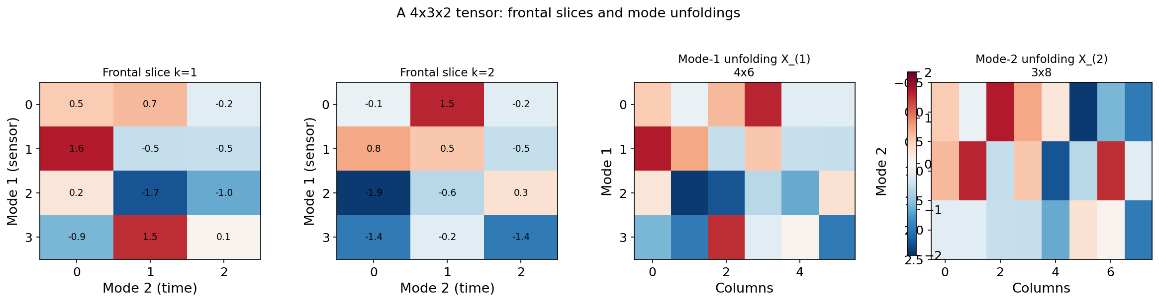
Mode- Unfolding (Matricization)
Definition 3 (Mode-n unfolding).
The mode- unfolding (or matricization) of , denoted , arranges the mode- fibers as the rows of a matrix. Each mode- fiber becomes a row of .
The unfolding connects tensor operations to matrix operations. In particular, the mode- product satisfies:
This identity — the matricization–mode product identity — is the bridge between tensor algebra and the matrix tools from the SVD and Spectral Theorem topics.
Tensor (4 × 3 × 2)
Unfolding
2. CP Decomposition (CANDECOMP/PARAFAC)
Definition and Rank
The CP decomposition expresses a tensor as a sum of rank-1 terms — the direct generalization of the matrix SVD’s outer-product expansion .
Definition 4 (CP decomposition and tensor rank).
An order- tensor has a CP decomposition of rank :
where denotes the outer product, each is a unit-norm factor vector, and is a weight. The tensor rank (or CP rank) is the minimum for which such a decomposition exists.
Comparison with the matrix SVD:
| Property | Matrix SVD | Tensor CP |
|---|---|---|
| Factors | (two sets of vectors) | ( sets) |
| Weights | , ordered | , unordered in general |
| Orthogonality | Not guaranteed | |
| Uniqueness | Up to sign | Essential uniqueness under mild conditions (Kruskal) |
| Best rank- | Always exists (Eckart–Young) | May not exist for tensors of order |
The last two rows are the fundamental surprises of tensor algebra. The CP decomposition is more unique than the SVD (no rotation ambiguity) but less well-behaved (best rank- approximation may not exist).
Kruskal’s Uniqueness Theorem
Definition 5 (Kruskal rank).
The Kruskal rank (or -rank) of a matrix , denoted , is the maximum value such that every subset of columns of is linearly independent. Note: , with equality when has full column rank.
Theorem 1 (Kruskal's uniqueness theorem (1977)).
Let be a rank- CP decomposition of an order-3 tensor, with factor matrices . If
then the decomposition is essentially unique: any other rank- decomposition is identical up to permutation and scaling of the rank-1 terms.
Proof.
Proof sketch. The condition ensures that the Khatri–Rao products have full column rank . The key observation is that if two CP decompositions represent the same tensor, then:
Unfolding along mode 1 gives . The Kruskal rank condition guarantees that the Khatri–Rao product has rank , making this system of equations solvable only when for a permutation matrix and diagonal scaling matrices with .
∎This is a remarkable result with no matrix analog. The matrix SVD is unique only up to rotation within eigenspaces of equal singular values — any orthogonal transformation , gives the same matrix . But under the Kruskal condition, CP factors are essentially unique: the individual rank-1 components are identifiable, not just the subspace they span.
Alternating Least Squares (ALS)
The standard algorithm for computing the CP decomposition is Alternating Least Squares (ALS). The idea: fix all factor matrices except one, then solve the resulting least-squares problem for that one. Cycle through all modes repeatedly until convergence.
For mode , the least-squares subproblem is:
where denotes the Khatri–Rao (columnwise Kronecker) product.
def cp_als(tensor, rank, max_iter=200, tol=1e-8, seed=42):
    """Alternating Least Squares for CP decomposition."""
    rng = np.random.RandomState(seed)
    N = tensor.ndim
    shape = tensor.shape

    # Random initialization
    factors = [rng.randn(shape[n], rank) for n in range(N)]
    for n in range(N):
        factors[n] /= np.linalg.norm(factors[n], axis=0, keepdims=True)
    weights = np.ones(rank)

    for iteration in range(max_iter):
        for n in range(N):
            # Khatri-Rao product of all factors except n
            V = khatri_rao_except(factors, n)
            Xn = unfold(tensor, n)

            # Normal equations: A^(n) = Xn @ V @ (V^T V)^{-1}
            VtV = np.ones((rank, rank))
            for m in range(N):
                if m != n:
                    VtV *= factors[m].T @ factors[m]
            factors[n] = Xn @ V @ np.linalg.pinv(VtV)

            # Normalize columns
            norms = np.linalg.norm(factors[n], axis=0)
            weights = norms
            factors[n] /= np.maximum(norms, 1e-12)

        # Check convergence
        recon = reconstruct_cp(weights, factors)
        error = np.linalg.norm(tensor - recon) / np.linalg.norm(tensor)
        if iteration > 0 and abs(prev_error - error) < tol:
            break
        prev_error = error

    return weights, factors, error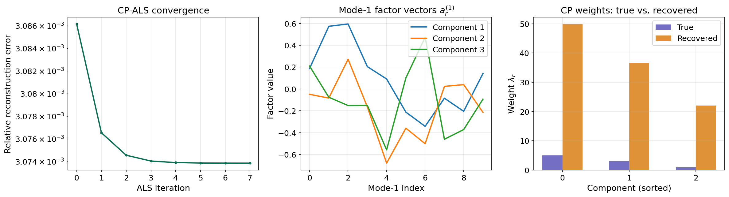
3. Tucker Decomposition
Definition and Multilinear Rank
The Tucker decomposition generalizes the matrix factorization by allowing a different rank reduction along each mode.
Definition 6 (Tucker decomposition).
An order- tensor has a Tucker decomposition:
where is the core tensor and each is a factor matrix (typically with orthonormal columns). The tuple is the multilinear rank.
Definition 7 (Multilinear rank).
The multilinear rank of is the tuple , where is the mode- unfolding. Unlike the matrix rank (a single number), the multilinear rank is an -tuple that can differ across modes.
Comparison: Tucker vs. CP:
| Property | Tucker | CP |
|---|---|---|
| Core | Full core tensor with interactions | Superdiagonal: only if |
| Parameters | ||
| Uniqueness | Up to rotation within each mode (like matrix SVD) | Essentially unique (Kruskal) |
The CP decomposition is a special case of Tucker where the core tensor is superdiagonal and .
Connection to PCA
The Tucker decomposition is precisely multilinear PCA. The factor matrix captures the principal subspace of the mode- unfolding — that is, PCA applied independently along each mode. The core tensor captures the multi-mode interactions between these subspaces.
Existence and Computation
Theorem 2 (Tucker decomposition existence).
Every tensor admits a Tucker decomposition with multilinear rank where . This decomposition is computed by setting to the left singular vectors of and .
Proof.
By the SVD, each mode- unfolding has a decomposition . The first columns of span the column space of , which contains all mode- fibers. Since the mode- fibers are the rows of , the tensor can be reconstructed from its projections onto these -dimensional subspaces along each mode. The core tensor stores the coordinates in these subspaces, and reconstruction follows from by the properties of the mode- product.
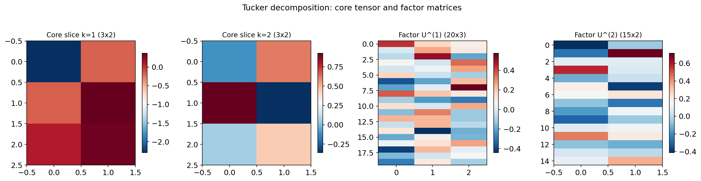
∎Factor matrices
Core tensor 𝒢 — frontal slices
Decomposition stats
- Relative error: 34.85%
- Compression: 14.1×
- Core entries: 8
- Factor entries: 60
- Total stored: 68 / 960
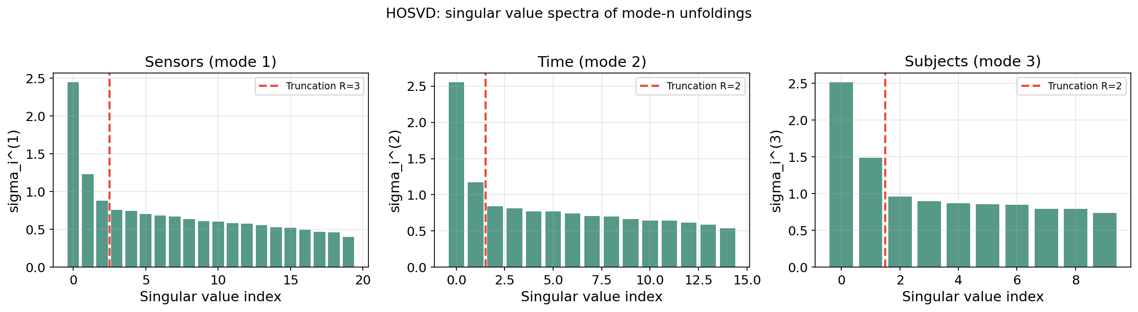
4. Higher-Order SVD (HOSVD)
Definition
The HOSVD (De Lathauwer, De Moor & Vandewalle, 2000) is a specific Tucker decomposition obtained by applying the matrix SVD independently to each mode- unfolding.
Algorithm (HOSVD):
- For each mode : compute the (truncated) SVD of the mode- unfolding .
- Set the factor matrix to (left singular vectors of ).
- Compute the core tensor: .
def hosvd(tensor, ranks=None):
    """Compute the (truncated) HOSVD."""
    N = tensor.ndim
    if ranks is None:
        ranks = tensor.shape

    factors = []
    singular_values = []
    for n in range(N):
        Xn = unfold(tensor, n)
        U, s, Vt = np.linalg.svd(Xn, full_matrices=False)
        factors.append(U[:, :ranks[n]])
        singular_values.append(s[:ranks[n]])

    core = tensor.copy()
    for n in range(N):
        core = np.tensordot(factors[n].T, core, axes=([1], [n]))
        core = np.moveaxis(core, 0, n)

    return core, factors, singular_values
Properties
Theorem 3 (HOSVD properties (De Lathauwer et al., 2000)).
The HOSVD satisfies:
- All-orthogonality: Each factor matrix has orthonormal columns.
- Ordering: The mode- singular values are non-negative and can be ordered: .
- Multi-mode interactions: quantifies the interaction between the -th pattern along each mode.
Key difference from the matrix SVD: The truncated HOSVD is not the best rank- Tucker approximation. The HOOI (Higher-Order Orthogonal Iteration) refines it to a local optimum.
Approximation bound: Let be the truncated HOSVD and the best Tucker approximation. Then:
This suboptimality factor is the price for the HOSVD’s simplicity — it computes each mode’s SVD independently rather than jointly optimizing all modes.
5. Tensor Train Decomposition
The Curse of Dimensionality in Tucker
The Tucker decomposition has a fundamental scaling problem. For an order- tensor with multilinear rank , the core tensor has entries — exponential in the number of modes. For a 10-way tensor with , the core alone has million entries.
The Tensor Train Format
Definition 8 (Tensor Train decomposition).
An order- tensor has a Tensor Train decomposition with TT-ranks where :
where each is a matrix obtained by fixing the “physical” index in the 3-way core tensor .
Storage comparison: For an order- tensor with all modes of size and rank :
| Format | Storage | ||
|---|---|---|---|
| Full tensor | 100,000 | ||
| Tucker | 393 | 59,349 + 300 | |
| CP | 150 | 300 | |
| Tensor Train | 450 | 900 |
Tucker’s core grows exponentially; TT grows linearly. The TT format trades a slightly larger per-mode cost ( vs. ) for freedom from the exponential core.
TT-SVD Algorithm
Theorem 4 (TT-SVD (Oseledets, 2011)).
Every tensor admits a TT decomposition. The TT-SVD algorithm computes it via a sequence of reshapes and SVDs:
- Start with .
- Compute the SVD: . Truncate to rank . Set .
- Set .
- Repeat: SVD, truncate, reshape.
Approximation bound:
where is the best rank- approximation of the -th intermediate matrix.
The TT-SVD is a sequence of matrix SVDs — each application of the Eckart–Young theorem controls one bond dimension. The total error accumulates at most additively, not multiplicatively.
def tt_svd(tensor, max_rank=None, tol=1e-10):
    """TT-SVD algorithm for Tensor Train decomposition."""
    N = tensor.ndim
    shape = tensor.shape
    if max_rank is None:
        max_rank = max(shape)

    cores = []
    C = tensor.copy().reshape(shape[0], -1)
    r_prev = 1

    for k in range(N - 1):
        C = C.reshape(r_prev * shape[k], -1)
        U, s, Vt = np.linalg.svd(C, full_matrices=False)
        r_k = min(max_rank, len(s))
        if tol > 0:
            r_k = min(r_k, max(1, (s > tol * s[0]).sum()))
        cores.append(U[:, :r_k].reshape(r_prev, shape[k], r_k))
        C = np.diag(s[:r_k]) @ Vt[:r_k, :]
        r_prev = r_k

    cores.append(C.reshape(r_prev, shape[-1], 1))
    return cores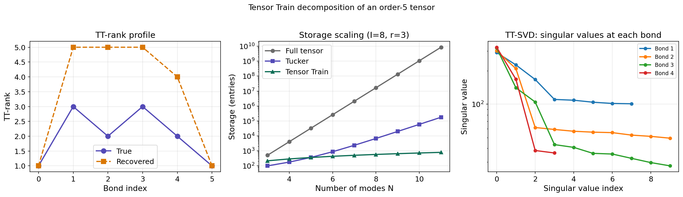
6. The t-SVD (Tensor SVD via the Fourier Domain)
Motivation
Can we define a tensor factorization with an exact Eckart–Young theorem? For order-3 tensors, the answer is yes. The t-SVD (Kilmer & Martin, 2011) defines a new algebra on 3-way tensors under which the SVD generalizes directly.
The t-Product
Definition 9 (t-product).
Let and . The t-product is computed by:
- DFT along mode 3: , .
- Multiply frontal slices: for each .
- Inverse DFT: .
The t-product transforms a tensor multiplication problem into independent matrix multiplications in the Fourier domain. This is exactly the structure we need to inherit the matrix SVD’s properties.
The t-SVD
Definition 10 (t-SVD).
Every has a t-SVD: where and are orthogonal (in the t-product sense) and is f-diagonal (only the diagonal tubes may be nonzero).
Definition 11 (Tubal rank).
The tubal rank of is the number of nonzero singular tubes in — equivalently, the maximum rank across all Fourier-domain frontal slices.
Optimal Approximation
Theorem 5 (Eckart–Young theorem for t-SVD (Kilmer & Martin, 2011)).
The truncated t-SVD is the best tubal-rank- approximation in the Frobenius norm:
Proof.
By Parseval’s theorem, . The tubal-rank- constraint corresponds to rank- constraints on each Fourier-domain frontal slice .
By the matrix Eckart–Young theorem applied independently to each , the optimal rank- approximation of keeps its top singular values and truncates the rest. The truncated t-SVD does exactly this: it applies rank- truncation to each Fourier-domain slice.
Since the Fourier transform preserves the Frobenius norm (Parseval), minimizing decomposes into independent matrix problems, each solved optimally by the truncated SVD. The inverse DFT recovers the optimal tensor approximation.
∎This is the only tensor decomposition with an exact Eckart–Young theorem. The CP decomposition’s best rank- approximation may not even exist (the infimum is not achieved). The Tucker/HOSVD approximation is within of optimal. The t-SVD achieves exact optimality by working in the Fourier domain, where the tensor problem decomposes into independent matrix problems.
def t_svd_truncated(tensor, rank):
    """Truncated t-SVD (best tubal-rank-k approximation)."""
    I1, I2, I3 = tensor.shape
    T_hat = fft(tensor, axis=2)

    recon_hat = np.zeros_like(T_hat)
    singular_values = []
    for k in range(I3):
        u, s, vt = np.linalg.svd(T_hat[:, :, k], full_matrices=False)
        r = min(rank, len(s))
        recon_hat[:, :, k] = (u[:, :r] * s[:r]) @ vt[:r, :]
        singular_values.append(s)

    return np.real(ifft(recon_hat, axis=2)), singular_values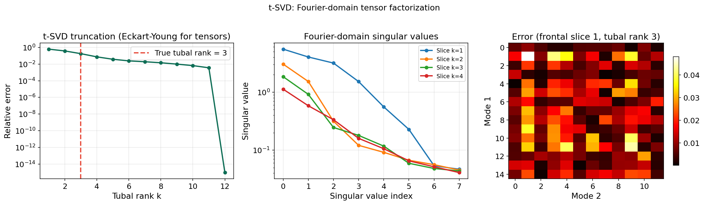
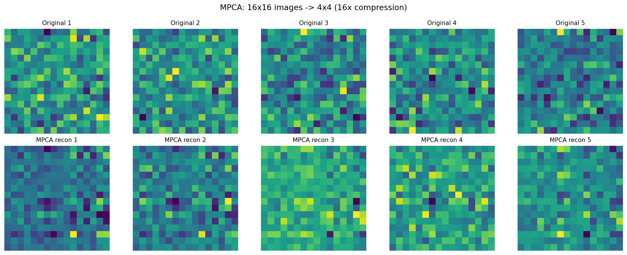
7. Multilinear PCA
From PCA to MPCA
PCA operates on vectors: each observation is a point, and PCA finds the -dimensional subspace of maximum variance. But when each observation is naturally a matrix or tensor, vectorizing destroys spatial structure and inflates dimensionality.
Multilinear PCA (MPCA) (Lu, Plataniotis & Venetsanopoulos, 2008) applies dimensionality reduction along each mode of a tensor dataset without vectorization.
Formulation
Given tensor observations with , MPCA seeks projection matrices maximizing the total scatter of the projected tensors. This is solved by alternating optimization: fix all projections except , project, unfold along mode , and apply standard PCA.
Connection to Tucker and HOSVD
MPCA is equivalent to computing the Tucker decomposition of the dataset tensor (observations stacked along an extra mode). The HOSVD initialization gives the starting point, and HOOI refines it. The PCA along each mode is the Spectral Theorem applied to the mode- scatter matrix.
8. Applications
8.1 Recommender Systems (CP)
A user × item × context tensor captures interaction data. The CP decomposition extracts latent factors — user preferences, item characteristics, and contextual effects — as separate vectors. Kruskal’s uniqueness theorem guarantees the factors are meaningful, not arbitrary rotations. This contrasts with matrix factorization (users × items), where PCA/SVD factors are unique only up to rotation.
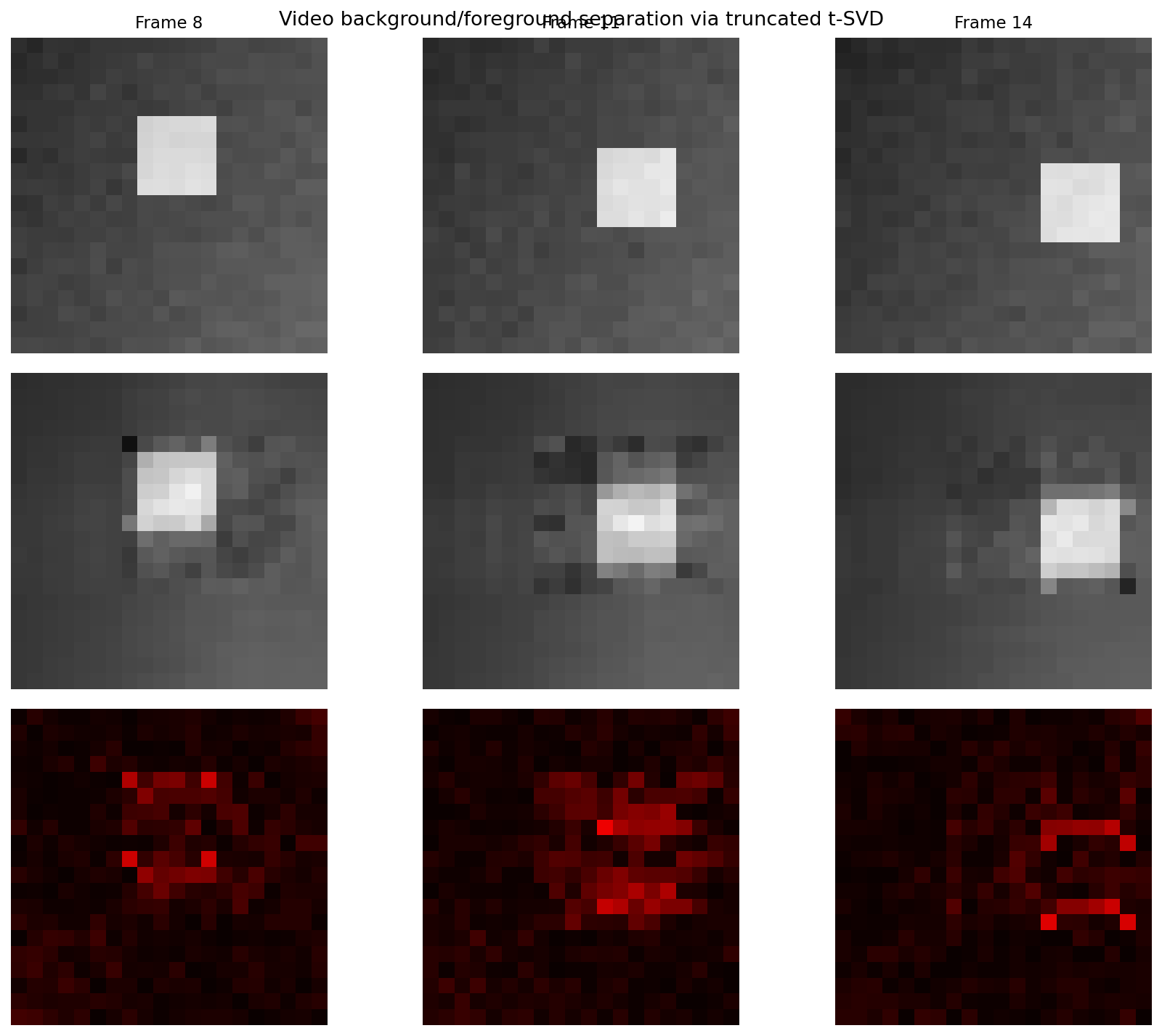
8.2 Video Surveillance (t-SVD and Robust Tensors)
A height × width × frames tensor represents video. The low-tubal-rank component captures the static background (via the t-SVD), while the sparse component captures moving foreground. This extends the matrix Robust PCA framework from 2D to 3D, preserving temporal correlations across frames.
8.3 Neuroimaging (Tucker/HOSVD)
EEG data (channels × time × trials × subjects) decomposes via Tucker into spatial, temporal, trial-level, and subject-level factors simultaneously. Each factor matrix captures the dominant patterns along its mode, and the core tensor reveals how spatial patterns interact with temporal dynamics across trials and subjects.
8.4 Quantum Chemistry (Tensor Train)
The wave function of an -electron system lives in a -dimensional space. TT/MPS compresses this to parameters, making quantum chemistry computations tractable for systems with tens of electrons — a problem where the Tucker core’s scaling is completely infeasible.
8.5 Topological Data Analysis
Persistent homology applied to tensor factor scores reveals topological structure in the latent factor space. The Mapper algorithm applied to CP factor scores produces topological summaries of tensor data. The bottleneck distance quantifies stability of topological features across tensor decomposition parameters (rank, regularization).
9. Computational Notes
Python Libraries
| Library | Decompositions | When to use |
|---|---|---|
tensorly | CP, Tucker, TT, Robust, Non-negative | General-purpose tensor decompositions |
numpy.einsum | Contractions, mode products | Low-level tensor operations |
scipy.fft | t-SVD implementation | Fourier-domain tensor computations |
opt_einsum | Optimized contractions | Large-scale tensor networks |
TensorNetwork (Google) | TT, MERA, general networks | Quantum-inspired tensor methods |
Complexity
| Method | Time complexity | Space |
|---|---|---|
| CP-ALS (order 3) | per iteration | |
| Tucker-HOOI (order 3) | per iteration | |
| HOSVD (order 3) | (three SVDs) | |
| TT-SVD (order ) | ||
| t-SVD |
Numerical Considerations
- CP rank determination: The tensor rank is NP-hard to compute. Use CORCONDIA (core consistency diagnostic) in practice.
- Degeneracy in CP-ALS: Factor vectors may become nearly collinear with opposite-sign weights. Regularization or non-negative constraints help.
- HOSVD as initialization: Always use HOSVD initialization over random initialization for Tucker decompositions.
- TT-rounding: After arithmetic in TT format, TT-ranks grow. Re-compress via sequential SVDs — analogous to matrix low-rank truncation from the SVD topic.
Einstein Summation
The np.einsum function provides a compact notation for tensor operations:
# Mode-2 product: X ×_2 B
result = np.einsum('ijk,lj->ilk', X, B)

# Tensor inner product: <A, C>
inner = np.einsum('ijk,ijk->', A, C)

# CP reconstruction: sum of outer products
recon = np.einsum('r,ir,jr,kr->ijk', weights, A, B, C)
10. Connections & Further Reading
The Tower of Factorization
The Linear Algebra track has built a tower of factorization:
- The Spectral Theorem: Symmetric matrices decompose into orthogonal eigenvectors.
- The SVD: Any matrix decomposes into orthogonal singular vectors with optimal truncation (Eckart–Young).
- PCA: The SVD of centered data yields dimensionality reduction, with extensions to nonlinear, probabilistic, robust, and sparse settings.
- Tensor Decompositions (this topic): Multi-way arrays decompose via CP (unique factors), Tucker/HOSVD (multi-mode PCA), Tensor Train (scalable to high order), and t-SVD (optimal truncation restored).
Each level generalizes the previous, and the Topology & TDA track provides tools for analyzing the topological structure of the resulting factor spaces.
Connection Table
| Topic | Connection to Tensor Decompositions |
|---|---|
| The Spectral Theorem (prerequisite) | The eigendecomposition of the mode- scatter matrices is the Spectral Theorem. The HOSVD applies it independently along each mode. |
| Singular Value Decomposition (prerequisite) | The HOSVD applies the matrix SVD to each mode unfolding. The t-SVD applies it to each Fourier-domain frontal slice. The TT-SVD is a sequence of matrix SVDs. |
| PCA & Low-Rank Approximation (prerequisite) | Tucker decomposition is multilinear PCA. MPCA applies PCA along each tensor mode. The scree plot generalizes to per-mode singular value spectra. |
| Persistent Homology (cross-track) | Persistent homology on tensor factor scores reveals topological structure in the latent factor space. Mode- singular value filtrations provide multi-scale persistence. |
| The Mapper Algorithm (cross-track) | Mapper applied to CP factor scores produces topological summaries of tensor data. |
| Barcodes & Bottleneck Distance (cross-track) | The bottleneck distance quantifies stability of topological features across tensor decomposition parameters. |
| Sheaf Theory (cross-track) | Sheaf Laplacian eigendecomposition on sensor networks produces multi-relational data naturally represented as tensors. Tucker decomposition of the sheaf cohomology tensor extracts multi-scale features. |
Summary Table
| Decomposition | Formula | Key property | Optimal approx? | Storage (order , size , rank ) |
|---|---|---|---|---|
| CP | Essentially unique (Kruskal) | No (may not exist) | ||
| Tucker | Multi-mode subspaces | HOSVD: within | ||
| HOSVD | Tucker via mode-wise SVD | Orthogonal factors, ordered | Within of optimal | |
| Tensor Train | Linear in | Error bounded | ||
| t-SVD | Eckart–Young analog | Yes (tubal rank) |
Connections
- The eigendecomposition of mode-n scatter matrices is the Spectral Theorem applied along each mode. The HOSVD computes it independently per mode. The Courant–Fischer minimax principle governs optimality of each mode's singular vectors. spectral-theorem
- The HOSVD applies the matrix SVD to each mode unfolding. The t-SVD applies it to each Fourier-domain frontal slice. The TT-SVD is a sequence of matrix SVDs. The Eckart–Young theorem generalizes to the t-SVD. svd
- Tucker decomposition is multilinear PCA. MPCA applies PCA along each tensor mode. The scree plot generalizes to per-mode singular value spectra. Kernel PCA extends to kernel tensor decompositions. pca-low-rank
- Persistent homology on tensor factor scores reveals topological structure in the latent factor space. Mode-n singular value filtrations provide multi-scale persistence. persistent-homology
- Mapper applied to CP factor scores produces topological summaries of tensor data. Mode-specific Mapper graphs using individual factor matrices as filter functions reveal per-mode topological structure. mapper-algorithm
- The bottleneck distance quantifies stability of topological features across tensor decomposition parameters (rank, regularization). Persistence barcodes of tensor factor spaces provide topological signatures. barcodes-bottleneck
- Sheaf Laplacian eigendecomposition on sensor networks produces multi-relational data naturally represented as tensors. Tucker decomposition of the sheaf cohomology tensor extracts multi-scale features. sheaf-theory
References & Further Reading
- book Tensor Decompositions and Applications — Kolda & Bader (2009) Comprehensive survey — CP, Tucker, properties, algorithms (SIAM Review)
- book Introduction to Linear Algebra — Strang (2016) Chapter 7: Matrix SVD foundations that tensor methods generalize
- book Matrix Analysis — Horn & Johnson (2013) Spectral theorem, Eckart–Young, and matrix norm properties used in tensor proofs
- paper A Multilinear Singular Value Decomposition — De Lathauwer, De Moor & Vandewalle (2000) Original HOSVD paper — defines the higher-order SVD and its properties
- paper Three-way arrays: rank and uniqueness of trilinear decompositions — Kruskal (1977) Kruskal's essential uniqueness theorem for CP
- paper Tensor-Train Decomposition — Oseledets (2011) TT-SVD algorithm and approximation bounds
- paper Factorization strategies for third-order tensors — Kilmer & Martin (2011) t-product, t-SVD, and Eckart–Young theorem for tensors
- paper MPCA: Multilinear Principal Component Analysis of Tensor Objects — Lu, Plataniotis & Venetsanopoulos (2008) MPCA formulation connecting Tucker to PCA
- paper Tensor Decompositions for Signal Processing Applications — Cichocki, Mandic, De Lathauwer, Zhou, Zhao, Caiafa & Phan (2015) Signal processing applications and modern tensor network methods