Normalizing Flows
Invertible neural networks for explicit-density generative modeling — from the change-of-variables formula to coupling layers (NICE/RealNVP), autoregressive flows (MAF/IAF), and Glow's multi-scale architecture, with the 2-moons worked example end-to-end
Motivation: explicit-density generative models
Generative modeling asks two questions about a distribution we cannot write down: can you draw a sample, and can you tell me how likely a given point is? The two questions sound symmetric but the methods that answer them are not, and the difference between them defines the major families of generative models in modern ML. This topic builds out the family that answers both questions with closed-form, exactly: normalizing flows.
What a generative model is asked to do
Suppose we have a dataset drawn from some unknown distribution on — images, audio waveforms, molecular structures, posterior samples from a Bayesian model, anything. A generative model is a learned object that tries to mimic , and the two operations we typically want from it are:
Sampling. Produce a fresh draw from the model’s distribution, where are the learned parameters. Cheap sampling is what makes a generative model useful as a data simulator, an imagination engine, or a proposal distribution for downstream Monte Carlo.
Density evaluation. Compute for an arbitrary point . Density evaluation is what makes a generative model useful as an anomaly detector, a likelihood-ratio building block, a compression scheme via Shannon coding, or a likelihood term for downstream inference.
A model that can do both operations cheaply and exactly is a strictly stronger object than one that can do only one. Almost all of the deep generative landscape splits on which of these two capabilities it sacrifices.
The VAE / GAN / flow trichotomy
Three families dominate generative modeling for continuous data.
Variational autoencoders (VAEs) pair an encoder with a decoder over a latent variable . They train by maximizing the evidence lower bound (ELBO), a lower bound on . Sampling is cheap (draw , push through the decoder). Density evaluation is bounded, not exact — marginalizing the latent to obtain is intractable, so we have the ELBO instead of the truth. The VAE pays for tractable training by accepting a bound.
Generative adversarial networks (GANs) train a generator against a discriminator that tries to tell real from generated. The generator is a sampler — push noise through, get a sample — but there is no density to query. GANs are implicit models: they parameterize the sampler directly and never write down a density. Sampling is cheap and often produces the sharpest synthetic outputs of any family. Density evaluation is unavailable.
Normalizing flows parameterize an invertible map that transforms a simple base distribution — almost always a standard Gaussian on — into the model distribution on the data space. Sampling means drawing and computing , a single forward pass. Density evaluation uses the change-of-variables formula
which is exact provided we can invert and compute the log-determinant of its Jacobian. The entire architectural project of normalizing flows is making these two operations cheap.
What flows offer that the other two families don’t is the conjunction: a sampler and an exact in one model. The cost is a fixed-dimension constraint (the input and output of every flow layer have the same dimension as the data, no bottleneck) and architectural design pressure to keep both and tractable. The next eleven sections are about how to discharge that pressure.
| Family | Sampling | Density evaluation | Training objective |
|---|---|---|---|
| VAE | Cheap, exact | Lower bound (ELBO) only | Max ELBO |
| GAN | Cheap, exact | Unavailable | Adversarial |
| Flow | Cheap, exact | Cheap, exact | Exact MLE |
The 1-D bimodal preview
Before formalizing anything, here’s the geometric picture flows operate by. Take a standard Gaussian on the line. Its density is the familiar bell. Now suppose our target is a two-mode mixture, — two narrow bumps centered at , with a valley in between. We’d like a smooth invertible map that pushes the Gaussian mass into the bimodal shape.
Geometrically, has to stretch the regions of the line where the target wants more mass (near ) and squish the regions where the target wants less (near and out in the tails). The change-of-variables formula will make this precise in §2: the Jacobian is exactly the local stretch factor, and the target density at is — the base density divided by how much stretched the neighborhood around . The whole machinery of flows is parameterizing the right and computing (or in higher dimensions) efficiently.
Roadmap
The plan from here:
- §2 derives the change-of-variables formula on in full, including the Jacobian-determinant volume-distortion factor. This is the only piece of math everything else builds on.
- §3 turns the formula into an architectural design constraint and shows how composing diffeomorphisms lets us build expressive flows from simple building blocks.
- §4 and §5 cover the two dominant flow architectures: coupling layers (RealNVP) and autoregressive flows (MAF / IAF). Both work by engineering a triangular Jacobian.
- §6 elaborates these for high-dimensional image data — Glow’s multi-scale architecture.
- §7 is the training recipe — maximum likelihood, no ELBO needed.
- §8, §9, and §10 cover what flows can express, how they plug into variational inference, and how they compare to nonparametric density estimation.
- §11 is the full worked example: a six-layer affine-coupling RealNVP on 2-moons, end-to-end, in 30 seconds of CPU time.
- §12 closes with applications, computational trade-offs, and the diffusion-model successor.
Change of variables in dimensions
The whole story of normalizing flows is downstream of one identity: when a smooth invertible map pushes a known density forward, the new density at the pushed-out point equals the old density at the pulled-back point, divided by how much stretched local volume. The 1-D version is calculus 101. The -dimensional version replaces “stretching” with “Jacobian determinant” — but the geometry is the same, and the proof is the same change-of-variables substitution we’d use to evaluate any multivariable integral.
The 1-D substitution rule as a geometric stretching factor
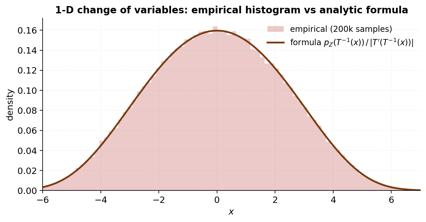
Start in one dimension. Let be a continuous random variable on with density , and let be a smooth, strictly increasing function. Define . We want .
The geometric reasoning is short. Consider a small interval in -space. maps this to — a small interval in -space of length . The probability mass in the input interval is ; the same mass has to land in the output interval (no probability appears or disappears under a deterministic map), so the density times the length of the output interval has to give back :
Solving for :
The factor in the denominator is exactly the local stretch factor: it tells us how much enlarged the neighborhood around . If , stretched the neighborhood, so the mass thinned out — the density at is smaller than at . If , compressed the neighborhood, so the mass piled up — the density at is larger than at .
When is decreasing rather than increasing, the same argument runs with in place of ; the absolute value handles the orientation flip. So in full generality:
Two readings of this formula sit side-by-side. The analytic reading: the density transforms via the substitution rule for integrals. The geometric reading: mass is conserved, and the density adjusts inversely to the local stretch. Both readings will generalize to in the next subsection — we just have to replace “local stretch” with “local volume distortion,” and the absolute value becomes the absolute value of a Jacobian determinant.
The -dimensional pushforward and the Jacobian-determinant volume distortion
Now lift to . Let have density , and let be a smooth bijection with smooth inverse . Define .
Theorem 1 (Change of variables for densities).
Under the conditions above, the density of is
where is the Jacobian matrix of at — the matrix whose entry is .
Proof.
For any bounded measurable function , the law of the unconscious statistician gives
Apply the multivariable substitution to the right-hand side. Under the substitution, , and the volume element transforms as — this is the multivariable change-of-variables theorem we are taking on as a load-bearing tool from formal calculus. The integral becomes
By definition , and equation (2.5) gives the same expectation in terms of an integrand involving and the Jacobian factor. Two integrals of the form agree for all bounded measurable if and only if almost everywhere, so
almost everywhere, which establishes the identity.
∎Equivalent forward form. Often it’s easier to evaluate the Jacobian of itself (the forward map) than of . The inverse-function theorem gives
and taking determinants on both sides:
Substituting into (2.3):
or equivalently, taking logs and writing :
Equations (2.3) and (2.9) say the same thing two ways. The implementation choice — Jacobian of the inverse (2.3), or Jacobian of the forward (2.9) — depends on which direction of the flow is easier to differentiate. Coupling layers (§4) and autoregressive flows (§5) both engineer the forward Jacobian to be triangular, so (2.9) is the form we’ll reach for in the architectural sections.
Geometric reading. The factor is the local volume-distortion factor: it tells us, locally near , how much the map scales infinitesimal -dimensional volume elements. A small box of volume in -space gets mapped to a small parallelepiped of volume in -space. The density adjusts inversely — mass is conserved, so where stretches volume, density thins; where compresses volume, density piles up. This is exactly the 1-D story from §2.1, lifted from intervals to volume elements via the Jacobian determinant.
Diffeomorphisms, the inverse-function theorem, and what fails without invertibility
The “smooth bijection with smooth inverse” condition in Theorem 1 is the definition of a diffeomorphism. Flows are parameterizing diffeomorphisms; everything in the architecture sections is engineered to keep that property under composition.
The local form is the inverse-function theorem: if is near and , then is a diffeomorphism on some neighborhood of , and its inverse satisfies the matrix identity (2.6). The global version — being a diffeomorphism on all of — is stronger than the local one, but for almost every flow architecture used in practice, is globally nonzero by construction (the affine-coupling Jacobian we’ll see in §4 is , strictly positive for all inputs), which combines with algebraic invertibility of the parameterization to give global invertibility.
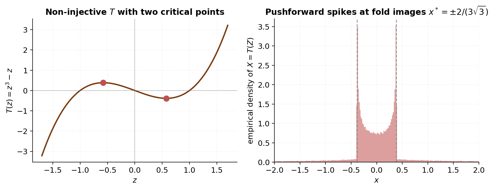
What goes wrong without invertibility is the geometric fold-and-density-blowup picture. Consider with — smooth, but not injective: , and the derivative vanishes at . Push a standard Gaussian through . Near , the inverse local-stretch factor blows up — equation (2.2) predicts an infinite density at the corresponding -values. This isn’t a bug in the formula; it’s a genuine pathology of pushing forward through a non-diffeomorphism. The pushed-forward measure isn’t even absolutely continuous near the fold points, so there is no honest density there at all.
For flow architectures, this pathology is what we have to avoid. Every layer must be a diffeomorphism with bounded away from zero on the parameter regime the optimizer can reach. §4 and §5 will show how the coupling and autoregressive parameterizations satisfy this automatically.
Numerical sanity: a linear map and a known closed-form pushed-forward density
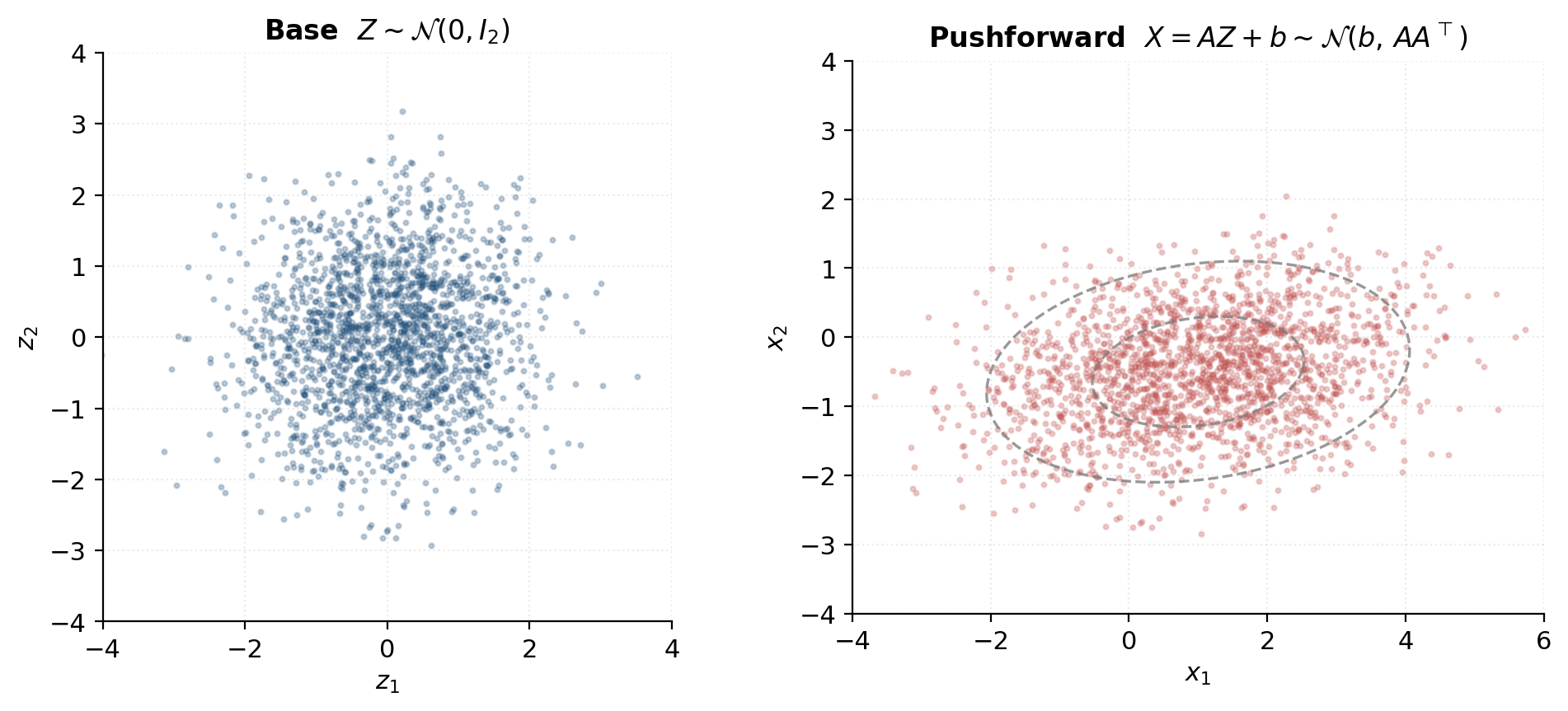
To check (2.3) against a known closed form, take the simplest possible case: a linear (well, affine) map. Let on , and define for fixed and . The forward map is ; its Jacobian is the constant matrix , so everywhere. The inverse is , with Jacobian , so .
Plugging into (2.3):
Substituting the standard-Gaussian density :
The exponent is a quadratic form. Using and :
This is exactly the density of — which is what we knew: a linear combination of independent Gaussians is Gaussian, with mean and covariance . The change-of-variables formula has reproduced the elementary fact, but importantly via the same machinery we’ll apply to flows where no closed form is available.
The notebook code computes both sides of (2.10) — the change-of-variables right-hand side using at the pulled-back point and the constant Jacobian factor, and the closed-form Gaussian density of via scipy.stats.multivariate_normal — for a batch of 1000 test points and confirms they agree to floating-point precision. This is the simplest sanity check we have on the change-of-variables formula; it also previews the structure of §4.3’s coupling-layer test, which computes a log-det two ways (closed-form vs autograd-Jacobian plus slogdet) and checks they match.
The normalizing-flow framework
Equation (2.3) tells us how a density transforms under a diffeomorphism. To turn this into a generative model, we need to (i) parameterize a family of diffeomorphisms rich enough to interpolate between any practical base and any practical target , and (ii) keep both the inverse and the log-det-Jacobian cheap enough that we can train by maximum likelihood and sample by forward evaluation. Those two requirements — invertibility and tractable log-det — are the entire architectural design pressure on flows. The rest of this topic is about meeting them.
Invertibility + tractable log-det as architectural pressure
Suppose for a moment we parameterized as an unconstrained multilayer perceptron — a fully connected network with ReLU activations, the standard workhorse. Two things go wrong.
Invertibility is not guaranteed. A ReLU MLP can collapse multiple inputs onto the same output: any that gets an all-negative pre-activation at the first layer maps to whatever bias the next layer carries forward, and many such exist. There is no architectural reason a generic MLP should be a bijection. We could try to detect non-invertibility post hoc, but training would have no signal to keep invertible — gradient descent on log-likelihood doesn’t see the invertibility constraint.
The Jacobian determinant is expensive. Even if were invertible, computing for a fully connected MLP costs — the determinant of a generic matrix requires LU decomposition or the equivalent. For (MNIST pixels), that’s billions of multiplications per evaluation, repeated for every training point in a batch and every step of optimization. The training loop is dead before it starts.
Flow architectures are engineered to dispatch both failures at once. The dominant trick is to constrain to be triangular (or block-triangular with simple blocks), so that the determinant is the product of the diagonal entries,
and the log-determinant is a sum over scalar logs — rather than . The two ways to engineer a triangular Jacobian — partitioning dimensions into “pass-through” and “transform” blocks (coupling layers, §4), and ordering dimensions autoregressively (autoregressive flows, §5) — are the two main flow architectures.
Invertibility comes along for the ride if the diagonal entries are always strictly positive. The triangular Jacobian then has positive determinant, the map is locally invertible by the inverse-function theorem, and the parameterization gives a closed-form inverse algebraically — by inverting the layer’s elementwise update rule, not by running a numerical solver. Coupling and autoregressive flows both produce strictly positive diagonal Jacobians by construction.
Composing diffeomorphisms — the log-det of a product is a sum
One simple flow layer is rarely expressive enough. We build expressive flows by stacking many layers and using the chain rule plus determinant multiplicativity to keep the log-det a sum of layerwise contributions.
Let where each is a diffeomorphism. Write and , so . The chain rule gives
a product of Jacobian matrices, each evaluated at the appropriate intermediate point. Taking determinants and using :
Taking logs of absolute values:
This is the composition rule for log-det-Jacobians. It has two consequences the architecture sections rely on:
-
Layerwise composition is additive in log-det. Doubling the depth of a flow doubles the per-layer log-det cost, but doesn’t introduce any cross-layer determinant computation. The log-det stays if each layer’s log-det is .
-
The inverse of a composition is the reverse composition of inverses. , with intermediate quantities , , and so on. If each layer’s inverse is closed-form and cheap, so is the composition’s.
Equation (3.4) is the engineering reason flows exist as a viable model class. We get expressivity by stacking; we don’t pay a determinant-of-a-product price for stacking.
The forward (sampling) direction and the reverse (density) direction
A flow has two distinct evaluation modes, and they’re not symmetric.
Forward (sampling). Draw , compute by applying each layer in turn. This is one neural-network forward pass per layer; if each layer is cheap to evaluate forward, sampling is cheap.
Reverse (density evaluation). Given , compute by applying the inverse of each layer in reverse order, then evaluate (equation (2.3) layered). This requires each to be cheap to evaluate, and each layer’s inverse log-det to be cheap.
For coupling layers (§4), both directions are cheap by construction — the inverse has the same arithmetic complexity as the forward, and the log-det is a sum of scalars either way. This is the property that makes coupling flows attractive: density evaluation and sampling are both parallelizable across the spatial dimensions.
Autoregressive flows (§5) are asymmetric. MAF makes density evaluation cheap (one parallel pass over dimensions) and sampling expensive (sequential, one dimension at a time). IAF inverts the asymmetry: sampling is cheap, density evaluation is sequential. The choice between the two depends on which direction the application calls more often:
- Density estimation / MLE training: density evaluation is in the hot loop, so MAF wins.
- Sampling-heavy applications (RL policies, image generation): sampling is in the hot loop, so IAF wins.
- Variational inference: the variational distribution needs both cheap sampling (to take Monte Carlo gradients of the ELBO) and cheap density evaluation of its own samples (to compute the entropy term). IAF was designed for this exact use case — see §9.
Coupling layers sit above the trade-off: both directions are cheap. The price they pay is in the partition structure (half the dimensions pass through every layer unchanged), which gets compensated for by stacking layers with alternating masks.
Why “normalizing”? The pushforward picture and the historical genealogy
The terminology can briefly trip up newcomers: “normalizing flow” doesn’t mean probability-normalizing (every density we write down is normalized by construction). It means transporting toward a normal distribution — toward specifically. The map takes data-space points and normalizes them to standard-Gaussian-distributed latents. Some authors call the “normalizing direction” and the “generative direction,” which makes the verb explicit.
The intuition is worth pausing on. Training a flow by MLE is equivalent to finding a diffeomorphism such that pushes the unknown data distribution as close to as possible — measured in KL divergence; see §7.1. At convergence, the residual non-Gaussianity of measures how well the flow has fit the data. This is a productive picture to keep in mind when looking at training curves and trained-flow diagnostics: a well-fit flow produces Gaussian-looking latent residuals, and the failure modes of flow training tend to be visible as residual non-Gaussianity.
Three historical waypoints anchor the framework:
-
Tabak and Vanden-Eijnden (2010) and Tabak and Turner (2013) introduced the construction in applied math as a nonparametric density estimator built from compositions of smooth invertible maps — no neural networks. Their motivation was numerical: cascade simple maps to slowly normalize a complicated density toward a tractable one.
-
Rezende and Mohamed (2015) brought the framework into deep learning, named it “normalizing flows,” and proposed planar and radial flows as the first neural-net-parameterized examples. Their use case was variational inference (§9): the family of variational posteriors that the ELBO can be optimized over is much larger if is a flow.
-
Dinh, Krueger, and Bengio (2014; NICE) and Dinh, Sohl-Dickstein, and Bengio (2017; RealNVP) introduced the coupling-layer construction, which made flows competitive as density estimators for high-dimensional structured data. Glow (Kingma and Dhariwal 2018) added 1×1 invertible convolutions and multi-scale architecture; MAF and IAF (Papamakarios, Pavlakou, and Murray 2017; Kingma et al. 2016) added the autoregressive variants.
The next two sections build the load-bearing architectures: coupling layers in §4, autoregressive flows in §5.
Coupling layers — NICE and RealNVP
Coupling layers are the dominant flow architecture in practice, for one reason: they make both directions (forward and inverse) cheap, with a closed-form log-det that costs the same as a single forward pass through a small MLP. The construction is a simple trick — partition the dimensions, transform half of them conditioned on the other half — but the trick produces a lower-triangular Jacobian, and once the Jacobian is triangular, the load-bearing math snaps into place.
Splitting dimensions with a binary mask and what each block does
Fix a binary mask . We’ll use the convention that marks dimension as pass-through (it goes through the layer unchanged) and marks it as transformed (it gets modified by an invertible scalar update conditioned on the pass-through dimensions). Let and be the two index sets, with .
The coupling layer takes input and produces output with the following block structure:
where is any invertible function parameterized by , and is the output of a neural network that takes only the pass-through dimensions as input. The key architectural fact is that the transformed dimensions depend on the pass-through dimensions but not on each other through the coupling layer (they may depend on each other through later layers, after the masks alternate).
The Jacobian of (4.1) has block-triangular structure. Order the dimensions so that comes first and comes second; then
where the upper-left block is the identity (pass-through dimensions), the upper-right block is zero (pass-through doesn’t depend on transformed), and the lower-right block is the Jacobian of with respect to its first argument (transformed-dim updates depend on transformed-dim inputs). The lower-left block is whatever it is — the transformed-dim updates depend on the pass-through inputs through , but the determinant doesn’t care because of the upper-right zero block.
Lemma (Block-triangular determinant).
For a square matrix of the form with and square, .
Proof.
Use the Leibniz formula , the sum over permutations of . Any that sends some row in the upper block to a column in the lower block hits the upper-right zero block at entry , and the corresponding term in the sum vanishes. The only surviving permutations are those that preserve the block structure: restricted to the upper block permutes the upper-block columns, and restricted to the lower block permutes the lower-block columns. The Leibniz sum factorizes over the two sub-permutations, giving .
∎Applying the lemma to (4.2) with and :
Now we just need to have a cheap log-det. The standard choice — both NICE and RealNVP make it — is for to act element-wise on , with each scalar update conditioned on :
With acting element-wise, is diagonal, and its determinant is the product of the diagonal entries.
Additive coupling (NICE): the simplest invertible nonlinearity
The simplest element-wise invertible is a shift:
where is an arbitrary neural network. This is additive coupling, introduced by Dinh, Krueger, and Bengio (2014) under the name NICE.
The Jacobian of (4.5) on the transformed block is the identity (each enters with coefficient ), so and (4.3) gives
NICE is volume-preserving — each layer has determinant exactly . This is appealing (no log-det term to track), but it limits expressivity: the entire pushforward can only redistribute mass, never concentrate or dilate it locally. NICE compensates by stacking many layers and adding a final non-volume-preserving diagonal rescaling.
The inverse of (4.5) is immediate: and for . The same network is used in both directions. Both forward and inverse cost one network evaluation.
Affine coupling (RealNVP): scale, translate, and the lower-triangular Jacobian
Affine coupling generalizes additive coupling by adding a scale factor:
where are neural networks (in practice, a shared trunk with two output heads). This is affine coupling, introduced by Dinh, Sohl-Dickstein, and Bengio (2017) under the name RealNVP — Real-valued Non-Volume Preserving.
The element-wise Jacobian on the transformed block:
so — a diagonal matrix with strictly positive entries. Plugging into (4.3):
and taking logs:
This is the load-bearing identity for coupling flows. The log-det-Jacobian is a sum of scalar outputs from the network — no matrix determinant computation, no autograd-on-the-Jacobian, just a sum over scalars the forward pass already computed. The cost of evaluating the log-det is essentially zero on top of the cost of evaluating and .
A few small points worth noticing. First, always (the exponential is strictly positive), so the affine coupling layer is always orientation-preserving and locally invertible by the inverse-function theorem. Second, the upper-left block in (4.2) doesn’t contribute to the log-det — the pass-through dimensions are free, in the sense that they cost nothing per layer. Third, expressivity per layer is bounded by the expressivity of and as functions of : a layer can scale and shift transformed dims as flexibly as and can vary across the pass-through input.
z_1 = -0.400
t(z_A) = -1.0120
log|det| = 0.3267
x_1 = -1.567
Stacking: alternating masks and why a single layer is not enough
A single coupling layer leaves dimensions unchanged. So a single layer cannot model any density whose marginal on the dimensions doesn’t match the base’s marginal — specifically, if and the target has a non-Gaussian marginal on dimension , a single layer with cannot fix that.
The fix is to alternate the mask between layers. Layer uses mask ; layer uses mask ; layer alternates back to ; and so on. After layers, every dimension has been transformed roughly times, and through the pass-through-to-transformed conditioning every dimension’s value depends on every other dimension.
For vector-valued data, the simplest alternation is the contiguous split and . For image data, the standard alternations are checkerboard masks (alternate pixels at the spatial scale) and channel-wise masks (alternate channels at the channel scale); Glow uses both at different scales of the architecture (§6).
The composition rule (3.4) applied to a stack of coupling layers gives
a sum over scalar outputs from the per-layer scale networks. Empirically, coupling layers suffice for 2-D toy targets like 2-moons (§11); image-scale flows like Glow use across multiple resolution scales (§6).
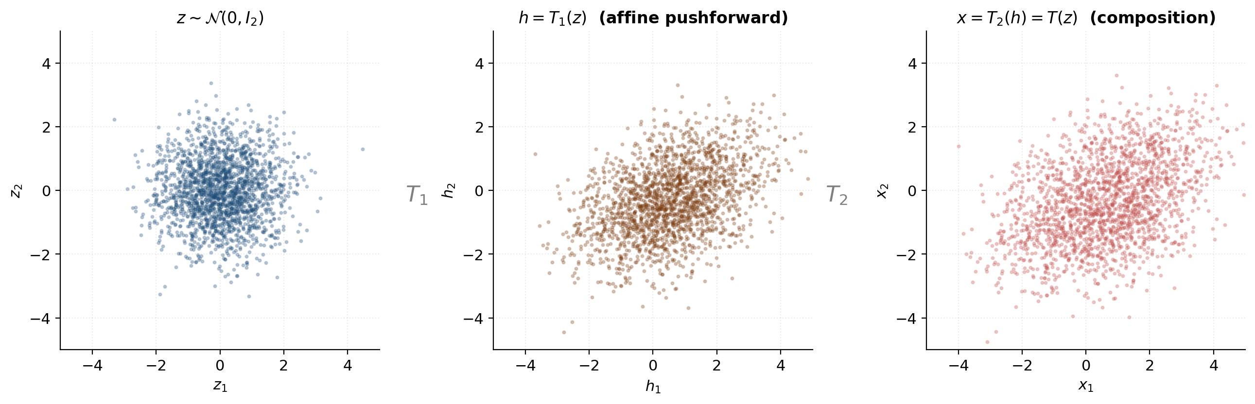
![Three-panel scatter showing the pushforward through a two-layer coupling stack: base Gaussian z ~ N(0, I_2) on the left, after layer 1 (mask [1, 0]) in the middle, and after layer 2 (mask [0, 1]) on the right.](/images/topics/normalizing-flows/04_coupling_stack_pushforward.png)
Inverse pass in closed form — and why this is the whole point
The inverse of (4.7) is closed-form:
Two things deserve emphasis. First, the inverse uses the same networks and — no separately-trained “inverse network.” The forward and inverse share parameters; what changes is the algebraic operation, not the function being learned. Second, the cost of evaluating is identical to the cost of evaluating : one forward pass through the MLP and one element-wise scale-shift (forward direction) or scale-divide-shift (inverse direction). For a stack of coupling layers, the inverse cost is MLP evaluations in reverse order — the same as the forward cost.
This is the property that gives coupling flows their dominance: density evaluation (which uses the inverse) and sampling (which uses the forward) are both , both parallelizable across the spatial dimensions, both differentiable end-to-end. Compare this to autoregressive flows (§5), where the forward and inverse have asymmetric costs by construction, and the reason RealNVP became the workhorse it did is immediate.
The log-det of the inverse, by (2.7), is minus the log-det of the forward at the corresponding point:
where we’ve used for any affine coupling layer (the pass-through dimensions are literally the same in and , so ).
Autoregressive flows — MAF and IAF
The same triangular-Jacobian trick that makes coupling layers work also produces a second major flow family: autoregressive flows. Where coupling partitions the dimensions into two fixed blocks and transforms one block conditioned on the other, autoregressive flows transform dimensions one at a time in a fixed order — dimension is updated conditioned on all earlier dimensions . The Jacobian is still lower-triangular, the log-det is still a sum of scalars, but the sampling-vs-density asymmetry becomes the architectural feature instead of being engineered away.
The autoregressive density decomposition
The chain rule of probability writes any joint density as a product of conditionals along an arbitrary ordering of the variables:
If we parameterize each conditional as a Gaussian,
the reparameterization trick gives sampling and density evaluation a single common form:
with independent across . The forward (sampling) map is ; the inverse is . Writing to ensure positivity, the forward update becomes
an affine update on each dimension conditioned on the earlier ones. (We’ve relabeled as for symmetry with §4.) Comparing with the coupling-layer update (4.7), the structural similarity is striking: both are element-wise affine maps with scale and shift . The difference is in what each update is conditioned on — fixed partition in coupling, growing prefix in autoregressive.
The Jacobian of in (5.4) is lower triangular: for (since depends on and on , which transitively depends only on ), and on the diagonal. The entries strictly below the diagonal are nonzero in general but irrelevant to the determinant. By the same triangular-determinant argument as §4.3,
Identical in form to the coupling log-det (4.10), with now being “all dimensions” and the conditioning being “everything before me” rather than “everything in the pass-through partition.”
MAF: parallel density evaluation, sequential sampling
Papamakarios, Pavlakou, and Murray (2017) introduced the Masked Autoregressive Flow (MAF) as the density-estimation specialization of (5.4). The defining equation is (5.4) verbatim: the scale and shift networks are conditioned on the data-side prefix (rather than the latent-side prefix ). This choice governs the computational asymmetry.
Density evaluation (parallel). Given , the entire prefix is observed for every — it’s just sliced from the input. All scale and shift outputs can be computed in a single forward pass through a masked autoencoder (MADE; Germain, Gregor, Murray, and Larochelle 2015), and the latents
are computed in parallel across . Log-density is then . Total cost: one MADE forward pass.
Sampling (sequential). Given , we want to compute by (5.4). But depends on , which we don’t yet have — we have , not . So we must compute first (using only , which have empty conditioning), then (using ), then (using ), and so on. Total cost: MADE forward passes, each conditioned on the cumulative output from the previous ones. The cost scales linearly in the data dimension, which becomes prohibitive at image scale ().
MAF is therefore the right choice when density evaluation is in the hot loop and sampling is rare — the canonical case being density estimation by maximum likelihood (§7), where every training step evaluates the log-likelihood on a batch and sampling is needed only at evaluation time.
IAF: parallel sampling, sequential density evaluation
Kingma, Salimans, Jozefowicz, Chen, Sutskever, and Welling (2016) introduced the Inverse Autoregressive Flow (IAF) by swapping the conditioning: condition on the latent-side prefix rather than the data-side prefix . The forward map becomes
This is the inverse of MAF in a precise sense: if we relabel the variables (, ), equation (5.7) is exactly equation (5.6) with sign-flipped scale. IAF is MAF run backward and renamed.
The computational asymmetry flips. Sampling (parallel): given , the entire prefix is observed for every , all compute in one MADE forward pass, and all are produced in parallel. Cost: one MADE forward pass. Density evaluation (sequential): given , the prefix depends on transitively, so we must invert dimension by dimension — sequential MADE passes.
IAF is the right choice when sampling is in the hot loop and the only density evaluation needed is on the model’s own samples — where is in hand alongside , so all the values are already computed during sampling and the sequential-density cost vanishes. This is the exact use case in variational inference, where the variational distribution is parameterized as an IAF: ELBO gradients require cheap sampling from and cheap log-density evaluation of those samples, both of which IAF delivers. §9 returns to this in detail.
The MAF↔IAF duality and when to reach for each
The trade-off table that summarizes the three flow families so far:
| Family | Sampling cost | Density-evaluation cost | Best for |
|---|---|---|---|
| Coupling (§4) | 1 forward pass | 1 inverse pass | Both directions cheap — default |
| MAF | sequential passes | 1 forward pass | Density estimation / MLE |
| IAF | 1 forward pass | sequential passes | Variational inference / sampling |
The duality is exact: the same MADE parameters trained as MAF can be evaluated as an IAF (and vice versa) by swapping the roles of input and output. In practice, IAF is trained via VI (where the model’s own samples are the only density queries it needs) and MAF is trained via MLE (where data-density queries dominate). The implementation choice is dictated by which side of the duality matches the training objective.
Stacking autoregressive flows uses the same alternation idea as coupling: after each layer, reverse the dimension ordering so that the “first” dim of the new layer is the “last” of the previous one. After layers with alternating orderings, every dim has been transformed conditioned on every other.
Coupling flows are the right starting point for most density-estimation problems because they’re cheap in both directions; autoregressive flows shine when one direction’s asymmetry matches the application’s access pattern. Glow (§6) elaborates the coupling design for images. Spline flows (Durkan, Bekasov, Murray, and Papamakarios 2019; §6.4 forward pointer) generalize the affine update inside a coupling or autoregressive layer to a piecewise rational-quadratic map, dramatically increasing per-layer expressivity without sacrificing tractability.
Multi-scale and image-domain architectures
The §4 and §5 architectures handle vector data with no spatial structure cleanly, but the original motivating use case for flows — image generation — needs more. An RGB image at resolution has dimensions; a single coupling layer on that would have an MLP with hundreds of millions of parameters and no inductive bias for the spatial locality of natural images. Glow (Kingma and Dhariwal 2018) introduced a small set of architectural primitives that make flows tractable at image scale by leveraging the same convolutional inductive biases as VAEs and GANs: squeeze for routing dimensions across spatial scales, 1×1 invertible convolutions for cheap channel mixing, and ActNorm for the invertible analog of batch normalization. None of these change the underlying flow math from §4 and §5 — they’re new building blocks that compose with coupling layers under the same change-of-variables formula.
The squeeze operation and dimension routing across scales
The natural way to scale a coupling flow on images is to operate at multiple spatial resolutions: the first few layers handle fine-grained pixel details, and later layers handle coarser-scale structure. This requires a way to route spatial dimensions into the channel axis without losing bijectivity.
The squeeze operation reshapes a tensor into a tensor by stacking spatial blocks along the channel axis. Concretely: every block of pixels in the input becomes a single column of channel values in the output. Each output channel at spatial position corresponds to a triple with via , and the new value is .
Squeeze is a permutation of the input dimensions. Its Jacobian is a permutation matrix — exactly one per row and column, zeros elsewhere. So and . Squeeze costs nothing in the change-of-variables accounting.
After a squeeze, a channel-wise mask (half the channels pass through, half get transformed) acts at the coarser spatial scale. Glow alternates squeeze with coupling-block sequences across scale levels: at each level the spatial resolution halves and the channel count quadruples, doubling the model’s “effective coverage area” per coupling layer. After the final scale level, the tensor is flattened and a small set of vector-valued coupling layers handles the remaining global structure.
Glow also uses a split operation between scale levels, where half the channels at each scale are peeled off and sent directly to the output (“factored out” in Glow’s terminology). This reduces the per-layer parameter count at deeper scales without sacrificing capacity — the factored-out dimensions get a Gaussian prior, and the remaining ones continue through the next scale’s coupling stack. Split is a partition, also a permutation under the change-of-variables — no log-det cost.
1×1 invertible convolutions — channel-mixing with closed-form log-det
Between coupling layers, we need to mix the channels so that subsequent couplings don’t act on the same fixed partition repeatedly. NICE and RealNVP used fixed channel permutations (alternate which channels are pass-through). Glow generalizes the fixed permutation to a 1×1 invertible convolution — a learnable matrix applied independently at every spatial position.
Forward: for every . The operation is identical to a fully connected layer applied at each pixel.
For the operation to be invertible, must be invertible (nonzero determinant). The Jacobian of the full operation on the flattened input is block-diagonal with copies of on the diagonal — one per spatial position. So
The challenge: computing for a generic dense matrix is via LU decomposition. For this is acceptable per call but adds up across many layers and many training steps.
Glow’s solution is the LU parameterization:
where is a fixed permutation matrix (initialized once, frozen), is lower triangular with ‘s on the diagonal (learnable, free parameters), is strictly upper triangular (learnable, free parameters), and is a vector of scale parameters (learnable, free parameters). The total parameter count is , matching dense .
By the block-triangular determinant lemma (§4.1) and :
so
The log-det is a sum of scalar logs — rather than . Glow’s contribution is not the LU decomposition itself (which is textbook) but the parameterization: making , , the free parameters means gradient descent never has to compute the LU factorization, just track the factor matrices directly.
In practice is constrained positive by reparameterizing with the actual learnable parameter; then trivially. Glow itself uses a sign-and-magnitude parameterization that allows negative , but the magnitude-only variant is what most reimplementations adopt — simpler, and the freedom to flip channel signs is already provided by and the off-diagonal parameters.
For sampling, the inverse can be computed once and cached — it’s a per-layer matrix that doesn’t change between batches. The cost is amortized across all sample-generation calls.
ActNorm — invertible normalization
Training deep flows benefits from normalization, but batch normalization is not invertible per-sample — its mean and variance depend on the current batch, so the function for a single sample depends on the other samples in the batch. The change-of-variables formula needs a deterministic per-sample transformation, so BN is structurally incompatible with flows.
Glow’s ActNorm is the invertible substitute:
where are learnable per-channel parameters (no batch dependence at inference time). Initialization is data-dependent: on the first batch seen during training, and are set to the per-channel mean and standard deviation so that the post-ActNorm activations are unit-Gaussian. After initialization, they’re updated by gradient descent like any other parameter.
The Jacobian of ActNorm is diagonal with entries (repeated across all spatial positions for each channel), so
to compute, like the LU-parameterized 1×1 convolution. The empirical benefit is the same as for BN — stabilized activations across depth — without the batch-dependence problem.
Forward pointer — spline flows (Durkan et al. 2019)
The affine update inside a coupling or autoregressive layer () has only two free parameters per dim: the scale and the shift . Spline flows (Durkan, Bekasov, Murray, and Papamakarios 2019) replace the affine update with a piecewise rational-quadratic monotone interpolant: the real line is partitioned into bins (typically ), and the per-bin parameters specify a monotone map between bin endpoints. The result is dramatically more expressive — free parameters per dim instead of — while remaining invertible, having a tractable closed-form log-det (the Jacobian is still element-wise on the transformed block), and maintaining both forward and inverse cost the same as affine coupling.
Spline coupling flows achieve density-estimation results competitive with autoregressive flows at coupling’s parallel-in-both-directions speed. They are currently the practical sweet spot for density estimation; the only reason this topic doesn’t derive them is that the rational-quadratic interpolation machinery is a substantial detour from the change-of-variables core. The same architectural primitives (coupling partition, log-det sum, alternating masks) apply unchanged; only the scalar update rule changes.
Other architectural variants worth knowing about but beyond this topic’s scope:
- Continuous-time flows (Chen, Rubanova, Bettencourt, and Duvenaud 2018; Grathwohl, Chen, Bettencourt, Sutskever, and Duvenaud 2019, FFJORD): replace the discrete stack of layers with a Neural ODE and use Hutchinson’s stochastic trace estimator for the log-det. §8.4 returns to these.
- Residual flows (Behrmann, Grathwohl, Chen, Duvenaud, and Jacobsen 2019): use Lipschitz-constrained residual blocks where guarantees invertibility; log-det is estimated via a power series.
For the worked example in §11 and the training story in §7, we’ll stick to RealNVP affine coupling — it’s the cleanest pedagogical baseline, and the spline / continuous extensions are easier to motivate once the affine case is fully internalized.
Maximum-likelihood training
Training a flow is straightforward: we have in closed form via change-of-variables (2.3), so we just minimize the empirical negative log-likelihood on training data. No ELBO. No adversarial discriminator. No auxiliary KL term. The §4 code already produces all the right log-dets; this section ties everything together and runs the first end-to-end training experiment.
The exact log-likelihood objective and why no ELBO is needed
Suppose we have a parametric flow with base distribution , and want to fit its pushforward to data drawn from an unknown distribution . Maximum likelihood estimation (MLE) chooses to maximize the empirical log-likelihood
For a flow, the change-of-variables formula (2.9) gives the exact log-density:
Substituting with and dropping the -independent constant, the empirical negative log-likelihood (NLL — the loss we’ll minimize) is
where is the latent representation of the -th data point.
Two terms drive the gradient:
- Latent norm penalty — pulls toward the origin. Geometrically, it asks the flow’s inverse to normalize the data to standard-Gaussian-distributed latents.
- Log-det term — pulls the local volume-distortion factor down (preferring contractive maps in the data’s neighborhoods).
These are in tension. Contracting at the data points expands there, which pushes outward, increasing . Equilibrium is exactly where has transported to — the “normalizing” picture from §3.4 in algebraic form.
KL minimization view. As , the empirical MLE objective converges to . Maximizing this is equivalent to minimizing the forward KL divergence
(the term doesn’t depend on , so it drops from the gradient). Forward KL pins the model where the data has mass: must cover every region covers, else the integrand blows up at those points and the KL is infinite. This is the mode-covering property of MLE — flows trained by MLE rarely miss a mode of the data, though they can over-smooth across narrow features.
Applying change-of-variables once more inside the expectation gives the dual:
The pushforward of under has to be close to standard Gaussian. “Normalizing flow” verbed: at convergence, normalizes the data.
Why no ELBO? Because (7.2) is exact. VAEs need an ELBO because marginalizing the latent variable is intractable — has no closed form for nontrivial decoders. Flows have no latent to marginalize: every has a unique pre-image , computable in closed form. The change-of-variables formula turns “intractable marginalization” into “tractable inverse + log-det” in one architectural step. That’s the whole architectural contract.
The training loop in PyTorch
The recipe is short enough to fit on a postcard:
optimizer = torch.optim.Adam(flow.parameters(), lr=1e-3)
for step in range(n_steps):
    x_batch = sample_data(batch_size)
    z, log_det_inv = flow.inverse(x_batch)
    log_p = base_dist.log_prob(z) + log_det_inv
    nll = -log_p.mean()
    optimizer.zero_grad()
    nll.backward()
    torch.nn.utils.clip_grad_norm_(flow.parameters(), max_norm=5.0)
    optimizer.step()
That’s all. No ELBO, no adversarial discriminator, no separate KL term — just empirical NLL, gradient descent, and the closed-form log-det that came for free in the §4 architecture.
The notebook trains a 4-layer affine-coupling RealNVP (CouplingFlow(d=2, n_layers=4, hidden=32)) on a 2-D bimodal target — two Gaussian blobs at with — for 2000 Adam steps at learning rate , batch size 256. Total runtime: roughly 4 seconds on a 2020-era CPU. The training NLL drops monotonically from initialization to within nats of the target’s negative differential entropy — the information-theoretic lower bound for any model.
![Training-curve plot: NLL vs Adam step, dropping from ~3.5 nats at initialization to ~1.93 nats at convergence (2000 steps), with the information-theoretic floor -H[p_data] ≈ 1.88 marked.](/images/topics/normalizing-flows/07_training_curve.png)
Numerical stability tricks
Standard practical tricks that show up across flow implementations:
Scale clamping. Without bounding the scale output, in the affine-coupling update (4.7) can explode when on bad initial inputs. The AffineCoupling class in §4 uses s = torch.tanh(s_raw) to keep , bounding . Empirically, this single line drops the training-instability rate by an order of magnitude.
Gradient clipping. Per-batch gradient-norm clipping (torch.nn.utils.clip_grad_norm_(flow.parameters(), max_norm=5.0)) prevents individual outlier samples from destabilizing training when their gradient norms spike. The default max_norm=5.0 is robust across most flow training setups; tighter clips help with very deep flows (depth > 30).
Base distribution choice. Standard Gaussian is the default and works for almost all data. Some applications use a uniform base on (for grid-discretized image data) or a learned mixture of Gaussians (for conditional generation), but those are application-specific tweaks, not general improvements.
Weight decay. Most flow implementations use no weight decay or very small ( to ) decay only on the MLP weights, never on the per-layer learned biases. Heavy weight decay cripples expressivity — the network needs to range freely to fit varying local volume distortions.
Numerical precision. Float32 suffices for production-scale training. The §4–§6 Jacobian-validation experiments used Float64 to distinguish closed-form log-dets from autograd log-dets at FP precision; this section’s training run stays at Float64 for consistency, but Float32 is the production choice.
Diagnostics: training curves, sample sanity, latent Gaussianity
Three things to check during and after training:
Training curve. The NLL should decrease monotonically (with some minibatch-sampling noise) and plateau. A flat-from-the-start curve indicates the model isn’t learning — usually an architectural bug (mask wrong, log-det not summed correctly) rather than a hyperparameter issue. A sudden NLL jump after apparent convergence is the gradient-explosion signature; the gradient clip should prevent it, but if it shows up, decrease the clip threshold.
Sample sanity. Draw , push through , scatter-plot against the training data. The samples should be visually close to the data distribution. A flow that fits log-likelihood well but produces visibly degenerate samples is the signature of MLE’s mode-covering bias — the model is “spending capacity” on hitting every data point and over-smoothing in the gaps between.
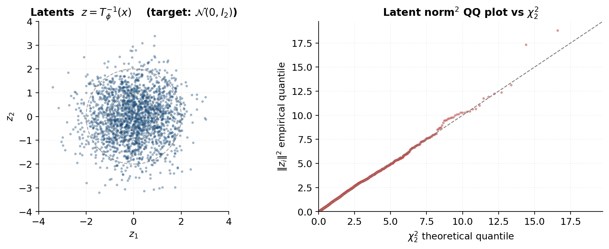
Latent Gaussianity. Compute for a held-out batch and check that the latents look like draws from . Two specific diagnostics:
- Latent scatter. should look isotropically Gaussian — no obvious clusters, no anisotropy, no banana shapes. Visible structure means the flow hasn’t fully normalized the data.
- Squared-norm QQ plot. Under perfect fit, follows (the sum of squared independent standard normals). Plotting empirical quantiles of against quantiles should fall on the diagonal. Deviations in the upper tail are common (outlier data points produce latents farther from the origin); deviations across the entire range indicate structural mis-fit.
Expressivity and universality
The training experiments in §7 fit a 4-layer RealNVP to a bimodal target without much effort, and the natural follow-up is: how far does this extend? Can a flow approximate any density on ? If so, how much depth and width do we need? And are there structural limits — densities that no finite affine-coupling flow can match? This section answers each question in turn.
What “universal” means for flows
The universality question for flows is: given a target density on , does there exist a diffeomorphism such that ? If yes, can it be approximated by the function class we’ve been studying — finite compositions of coupling layers with neural-net and ?
Two complementary results from measure-transport theory answer yes:
Existence (Bogachev, Sudakov). For any two atomless probability measures on , there exists a measurable map with . If both measures are absolutely continuous with everywhere-positive densities, can be taken to be a diffeomorphism. So some diffeomorphism exists transporting to any reasonable target — the remaining question is whether our parameterized family approximates it.
Constructive (Knothe–Rosenblatt rearrangement). For any two distributions with everywhere-positive densities, there is a unique triangular transport sending to . It’s built dimension by dimension via conditional inverse CDFs:
This is literally the autoregressive flow architecture from §5, with the optimal conditioning. So MAF and IAF, in the limit of infinite-width MLPs in each conditional, can exactly represent the Knothe–Rosenblatt map and hence approximate any target density.
Coupling flows are a slight restriction (they alternate which dims are “earlier” via masks, rather than fixing a single ordering), but Teshima et al. (2020) prove that affine-coupling flows with sufficient depth are also dense in the space of diffeomorphisms on any compact subset of , under mild regularity conditions. The proof constructs a finite stack of coupling layers that approximates a given target diffeomorphism uniformly on a compact set.
What “universal” doesn’t mean: it doesn’t mean any finite flow fits any density. There’s always an approximation error that depends on depth, width, and how well the MLPs can approximate the local affine coefficients of the Knothe–Rosenblatt map. The universality theorems guarantee the error goes to zero in the limit; they don’t tell us how fast.
Depth vs width and the empirical sweet spot
For practical flow training, the question becomes: how many coupling layers and how wide an MLP do we actually need? Theory gives bounds but not tight constants; the empirical answer comes from sweeping.
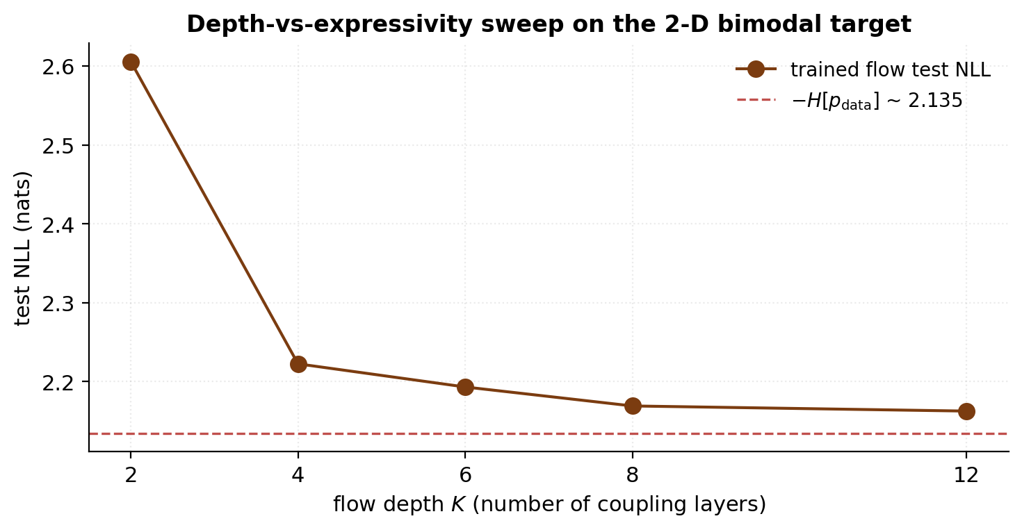
The notebook trains flows of depth on the §7 bimodal target — same training schedule, same data sampler, same architecture except for depth — and plots the final test NLL against depth. The standard pattern emerges: NLL drops sharply from to , then continues decreasing with diminishing returns. By the gap from the information-theoretic floor is under nats; by it’s under . The marginal benefit per extra layer flatlines.
This pattern generalizes. For 2-D toys, – is the practical sweet spot. For 10–50-dim density estimation (UCI tabular benchmarks; Papamakarios, Pavlakou, and Murray 2017), –. For image data at , across multiple scales (Glow’s published configuration). The depth scaling is roughly logarithmic in data complexity: doubling the per-dim conditional flexibility you can approximate requires roughly doubling the depth.
Width — the hidden dim of the MLP — has its own diminishing-returns curve. The §7 experiment used ; widths produce final NLLs within on the bimodal target. Width matters more when the conditioning network has to express complicated functions of (the conditional CDF of a multimodal target conditional on one of its modes, for instance) and matters less for smooth unimodal targets.
The rough heuristic: pick depth based on data dimensionality, width based on conditional complexity, and verify empirically on a small training run before scaling up. The hyperparameter space is forgiving — coupling flows aren’t fragile to depth or width in the way that some VAE / GAN architectures are.
Coupling-layer geometry: the topological barrier between disconnected modes
There’s a structural limit that universality theorems don’t address: diffeomorphisms preserve topology. The pushforward of a connected support under a diffeomorphism is connected; the pushforward of a simply-connected support is simply connected; and so on. The base distribution has all of as its support — fully connected and simply connected — so any diffeomorphism’s pushforward inherits both properties.
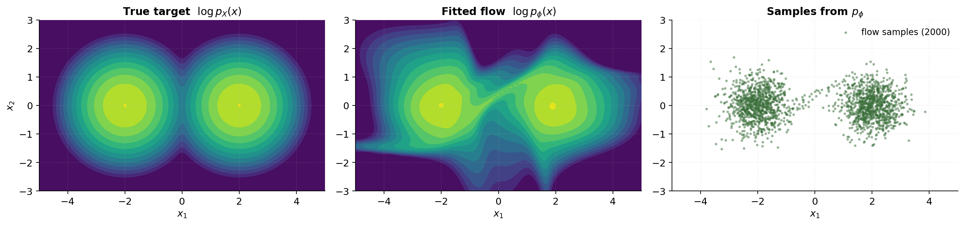
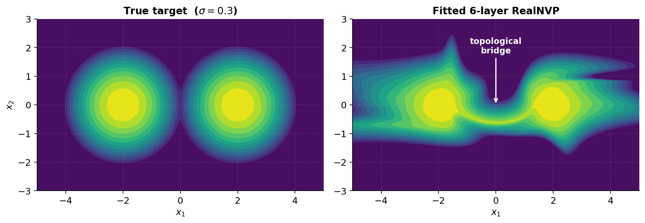
For practical mixtures with (Gaussian blobs that are formally connected — every point has positive density), this isn’t a hard barrier: the density between modes is low but not zero. However, the diffeomorphism nature of the flow forces the pushforward density to vary smoothly in space. A coupling-flow cannot make the bridge between modes arbitrarily low: it has to spend representational capacity on the corridor between blobs.
The empirical signature is a bridge of moderate density along the line connecting two modes in the fitted-density heatmap. The notebook re-trains a 6-layer RealNVP on a target (sharper modes than §7’s ), and the fitted heatmap shows a faint corridor between the two centers that the true density doesn’t have. This isn’t a training failure — it’s the topological constraint manifesting.
How modern variants partially address it:
- Spline flows (Durkan et al. 2019). The piecewise rational-quadratic monotone update inside each coupling layer can have very sharp gradients between bin endpoints, effectively concentrating the bridge into a thinner region. Still a diffeomorphism, but the effective topological barrier is much smaller.
- Continuous-time flows (FFJORD; §8.4). At any finite integration time the map is a diffeomorphism, so the barrier formally holds. But the ODE solver can integrate to very long times, producing maps with very steep gradients — the same “effective sharpness” benefit as spline flows.
- Hybrid models. Some practical implementations combine a flow with a discrete latent (a learned mixture-of-Gaussians base distribution, or a categorical latent that selects between component flows). The discrete latent contributes the disconnected-support structure; the flows contribute the smooth deformation within each component.
Affine-coupling flows can’t break the topological barrier alone, and that’s a meaningful structural limit. For unimodal or weakly-multimodal targets, it’s invisible. For data with genuinely discrete structure (categorical mixtures, isolated submanifolds), it’s a problem.
Forward pointer: continuous-time flows and FFJORD
The architectural successor to discrete-layer flows is the continuous-time family. Chen, Rubanova, Bettencourt, and Duvenaud (2018) — Neural Ordinary Differential Equations — replaced the discrete stack with a continuous ODE:
The log-det generalizes from the discrete sum (3.4) to an integral via the instantaneous change-of-variables formula (Chen et al. 2018, Theorem 1):
The trace of the Jacobian is an order cheaper than the determinant — to compute exactly, vs for the determinant. FFJORD (Grathwohl, Chen, Bettencourt, Sutskever, and Duvenaud 2019) brought it to stochastically via Hutchinson’s trace trick:
an unbiased estimator requiring only a single vector-Jacobian product per sample.
Continuous flows trade architectural simplicity for compute cost: each forward pass requires adaptive ODE integration (typically 10–50 RK4 steps per training example), which is 10–50× slower than a discrete flow with comparable expressivity. The trade-off pays off for high-dimensional density estimation, where FFJORD’s per-layer flexibility allows comparable quality with much shallower stacks; for low-dimensional toys like the §7 bimodal target, discrete coupling flows are strictly faster and equally good.
Continuous flows is its own follow-up topic — the Neural ODE machinery, adjoint-method backpropagation, and Hutchinson trace estimation each have enough depth to warrant a dedicated treatment. This topic forward-points to them as the natural next step for readers who hit the expressivity wall of discrete coupling flows.
Flows for variational inference
Normalizing flows were introduced to deep learning as variational distributions — Rezende and Mohamed’s 2015 paper that coined the name “normalizing flow” is a VI paper, not a density-estimation paper. The use case is straightforward: VI needs flexible variational families that can sample cheaply and evaluate their own density on their samples cheaply, and flows deliver both. The math is the same change-of-variables formula we’ve used since §2, applied with a slightly different sign convention — and that sign convention is the section’s main payoff.
This section is a bridge, not a full VI derivation. We assume the reader has seen the ELBO before (Variational Inference on this site; or, from the statistics side, formalStatistics’s Bayesian-computation chain) and focus on what’s specifically flows-y. The complete derivation of the ELBO, the reparameterization trick, and the standard choice of Gaussian variational families lives upstream.
Recap: the ELBO with a flexible
For a probabilistic model with intractable posterior , variational inference posits a tractable family and chooses to make close to . The evidence lower bound (ELBO) is
a lower bound on with equality iff . Maximizing the ELBO over both tightens the bound and minimizes the reverse KL divergence .
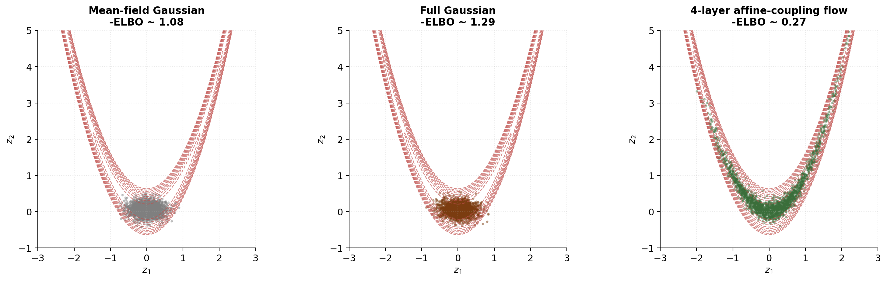
The expressive power of matters. Mean-field assumes posterior independence across components — usually wrong, often badly. Gaussian assumes posterior Gaussianity — also usually wrong but harder to detect. Both miss curved posterior structure: banana-shaped, multimodal, or heavy-tailed posteriors all break the Gaussian assumption.
Flows offer a flexible alternative.
Flow-augmented variational posteriors (Rezende & Mohamed 2015)
Parameterize the variational distribution as a flow:
where is an invertible flow whose architectural details may depend on the data point (the amortized setting; §9.4) or may be unconditional (when we’re approximating a single fixed target; the §9 code experiment). The variational distribution is then the pushforward of under :
or equivalently, substituting and using (2.7):
Equation (9.4) is the §2 change-of-variables formula, applied to a variational distribution instead of a generative model. The same architectural primitives — coupling layers, autoregressive flows, multi-scale convolutions — work unchanged.
Why use a flow as instead of for the model ? Two reasons. First, flexibility: a curved, multimodal, or heavy-tailed posterior is exactly the kind of thing a flow can match and a Gaussian cannot. Second, density-evaluation efficiency: VI training requires evaluating on samples drawn from itself, which means is in hand alongside . So (9.4) is essentially free: we already computed when sampling, and we already computed as part of the forward pass. This is the IAF use case (§5.3): cheap sampling and cheap density evaluation on the model’s own samples — exactly what VI wants.
The sign flip — entropy via change of variables
Here’s the part that’s productively confusing the first time through. The ELBO contains the entropy term , and the log-det shows up there with the opposite sign from §7’s density-evaluation case. Working it out carefully:
The entropy of is
Using the change of variables to push the expectation back to -space:
Substituting (9.4):
The entropy of the flow’s distribution equals the entropy of the base distribution PLUS the expected log-det of the forward Jacobian. Compare with §7’s density evaluation (7.2):
The log-det appears with a minus sign in the density formula and a plus sign in the entropy formula. Same term, same point, opposite signs. This is the sign flip.
The reason is bookkeeping, not magic: density is , entropy is , and the minus in the entropy definition flips the minus in front of the log-det. Geometrically the two readings are consistent:
- A flow that stretches volume locally (large ) reduces density at the pushed-forward point (the same mass spread over a larger region).
- The same flow increases entropy of the resulting distribution (more spread = more uncertainty = higher entropy).
The arithmetic agrees with the intuition. Once you see the sign flip once, you can read every flow-VI paper without flipping signs in your head.
The flow-VI ELBO. For an unobserved-data setting where we fit a flow to a fixed target :
Dropping the -independent constants ( and the unknown ), maximizing the ELBO is equivalent to minimizing
Two terms drive the gradient:
- — push the flow’s samples toward high-density regions of (low-potential regions).
- — penalize contracting maps; equivalently, reward spreading the distribution (entropy regularization).
These are in tension: the first pulls samples to the mode, the second prevents collapse. Equilibrium is the variational approximation. And we never need to know , the unknown normalizing constant of the target — a key advantage of VI over methods like rejection sampling that need normalized targets.
Amortized inference: encoder + flow as a practical pattern
In a standard VAE, the encoder produces for a Gaussian . To use a flow as , the encoder produces a context vector that conditions the flow’s networks:
The flow’s behavior — which regions it stretches, which it compresses — changes per data point through , and the joint encoder, flow parameters are trained by maximizing the ELBO across the training set. This is the amortized inference pattern.
Two production examples worth naming:
-
IAF-VAE (Kingma, Salimans, Jozefowicz, Chen, Sutskever, and Welling 2016). The variational posterior is an IAF whose autoregressive networks condition on the encoder output. IAF was designed for this use case: cheap sampling from for the ELBO’s MC gradient, cheap density evaluation on those samples for the entropy term, and the data conditioning lives in the encoder rather than in the flow’s architecture.
-
Sylvester flows (van den Berg, Hasenclever, Tomczak, and Welling 2018). Use a sequence of rank- flow updates ( with ), achieving a richer variational family than IAF at comparable compute cost. Less popular than IAF in practice but a useful comparison point.
The §9 code experiment uses the unconditional case (no encoder, no data-dependent conditioning) — fit a flow to a single fixed banana-shaped target . This isolates the flow-VI mechanics without the encoder-architecture complications. The amortized version is structurally identical: add a context vector to each MLP’s input, train end-to-end, repeat.
Flows for density estimation
This section is positional. §7 covered how to train a flow by maximum likelihood; this section covers where flows sit in the broader density-estimation landscape — what’s gained and what’s lost relative to the classical nonparametric and parametric alternatives, and what bridges this work to the wider neural function-approximation toolkit.
Neural-parametric density estimation and what it inherits from MLE
Density estimation — recovering from a sample — has two classical regimes. Parametric methods assume the target lies in a finite-dimensional family and estimate at the standard rate. Nonparametric methods make weaker smoothness assumptions and trade slower convergence for the absence of model misspecification. Flows are a third option that combines the parametric machinery (gradient-based fitting, rate within the representable family) with the flexibility of a high-dimensional, learned parameterization — neural-parametric density estimation.
The §7 MLE recipe is the inheritance from classical parametric statistics. Under regularity conditions — the true density is in the flow’s representable family, or is approximated arbitrarily well by it — the empirical MLE estimator is consistent ( as ) and asymptotically efficient (the variance reaches the Cramér–Rao bound). The flow’s expressive capacity — depth , width , layer type — controls the bias of the procedure: more capacity, less bias, but more variance for fixed .
The bias-variance trade-off has a familiar shape. Tiny flows () systematically underfit complex targets; huge flows () overfit small samples. The sweet spot is empirically the depth where validation loss stops decreasing — the usual hyperparameter-selection picture, but it pays off with the parametric convergence rate.
Contrast with KDE: bandwidth selection, rate of convergence, finite-sample regime
formalStatistics: Kernel Density Estimation takes a fundamentally different approach. Rather than fitting a parametric family, KDE places one kernel function per training point:
where is a kernel (often ) and is a bandwidth selected by cross-validation or Silverman’s rule. The estimator interpolates the empirical distribution, smoothing it by .
KDE’s convergence properties are nonparametric. For a -Hölder smooth target ( for targets — the standard assumption), the minimax rate in is
For :
- :
- :
- :
- : — barely any improvement with more data
This is the curse of dimensionality for nonparametric density estimation: the rate degrades polynomially in . To halve the error in requires more data; in , more.
Flows trade this for a parametric rate. Within the representable family, , independent of . The catch: the approximation error of a fixed-architecture flow is a bias that doesn’t shrink with — only with more flow capacity.
In practice:
- For low () and modest , KDE is often competitive or better — no model-misspecification bias, and the curse is mild.
- For high () or large , flows dominate — the curse hits KDE hard, and the flow’s approximation bias becomes a smaller fraction of the total error.
- The crossover depends on the data’s smoothness, the flow’s capacity, and the sample size.
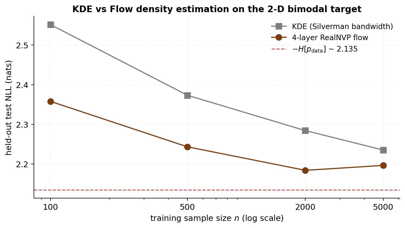
The notebook compares flow MLE against KDE on the §7 bimodal target (, ). The empirical pattern: KDE leads at (the flow doesn’t have enough data to estimate its parameters), they cross around , and the flow approaches the information-theoretic floor faster than KDE for .
Contrast with mixture models: flexibility, identifiability, mode merging
Gaussian mixture models (GMMs) are a finite-mixture parametric family:
GMMs are trained by expectation–maximization (EM): alternating between responsibilities (E-step) and component-parameter updates (M-step). Standard, cheap, and well-understood for up to a few hundred.
But GMMs come with three known pathologies:
- Model selection on . is a hyperparameter that must be set. Too few → underfit; too many → some components collapse (zero-variance singularity at a data point) or merge with others. Approaches like BIC and AIC trade off fit against complexity but don’t fully resolve the problem.
- Discontinuous gradients at the mode-merging boundary. When is held fixed but one component’s weight approaches , the effective model lies at the boundary of the lower- family. Standard gradient descent on this objective fails because the gradient with respect to that component’s parameters becomes ill-defined; EM handles it gracefully (responsibilities go to zero) but gradient-descent training does not.
- Local optima. The EM objective has many local optima for . Initialization matters, and standard random init often fails.
Flows avoid these. Their architecture has a fixed depth , but unlike GMM’s , depth is a continuous capacity dial — adding a coupling layer smoothly enriches the representable family without discontinuities. The MLE objective is smooth in . Local optima exist but are typically less problematic than for EM on GMMs (over-parameterization helps).
What flows lose: GMMs are interpretable. Each component has a mean and covariance you can read off, point to as a “cluster,” correspond to known data subpopulations. Flows are opaque — the learned networks don’t admit easy semantic interpretation. For data where the latent structure is genuinely a small number of Gaussian clusters, GMMs are arguably the right tool; flows are the right tool when the data’s structure is smooth, continuous, and not naturally decomposed into discrete components.
What flows can represent that GMMs cannot:
- Smooth manifold structure — the parabolic ridge of §9’s banana is a 1-D structure in 2-D space, not a small number of components. A GMM approximating it needs many narrow components along the ridge; a flow follows the ridge with a smooth diffeomorphism.
- Heavy tails without artifacts — a GMM approximating a Student- needs many components in the tails to track the slow polynomial decay; a flow on top of a Student- base captures it exactly with one layer.
- Correlation structure that doesn’t decompose — non-elliptical, non-mixture covariance patterns (think: the conformations of a folded protein, or the joint distribution of pixel intensities in natural images) where there’s no natural cluster boundary to define a mixture component over.
Bridge to density-ratio estimation
A common ML task is estimating the ratio rather than the density itself. Use cases include:
- Classifier two-sample testing: determining whether two empirical samples are from the same underlying distribution.
- Importance sampling: weighting samples from to estimate expectations under when sampling from is expensive.
- GAN discriminator: the Bayes-optimal discriminator estimates , and the GAN training objective is a moment-matching variant.
- Energy-based models: trained by contrasting positive samples (from ) against negative samples (from a noise distribution ).
The naive approach is to fit two flows separately and take the ratio . Two problems: each flow has its own approximation bias and variance (the ratio compounds both), and small errors in at low-density points produce huge errors in the ratio (division by a near-zero estimate).
The better approach is direct density-ratio estimation: train a single neural function that estimates without going through the densities individually. Two main families: (a) probabilistic classifier-based DRE, where a classifier distinguishing from samples gives log-odds that estimate ; (b) density-ratio matching via Bregman divergence between true and estimated ratios.
Both approaches inherit the parametric machinery from neural-network training and avoid the curse of dimensionality. They’re the subject of the T3 topic Density Ratio Estimation (coming soon) — the natural follow-up to flows for density estimation. The shared methodology (neural function approximation, MC training, similar diagnostics) makes the two topics natural companions, and both occupy the seven-topic PyTorch/JAX exception list for the same reason: neural-network parameterization with custom losses requires modern autodiff.
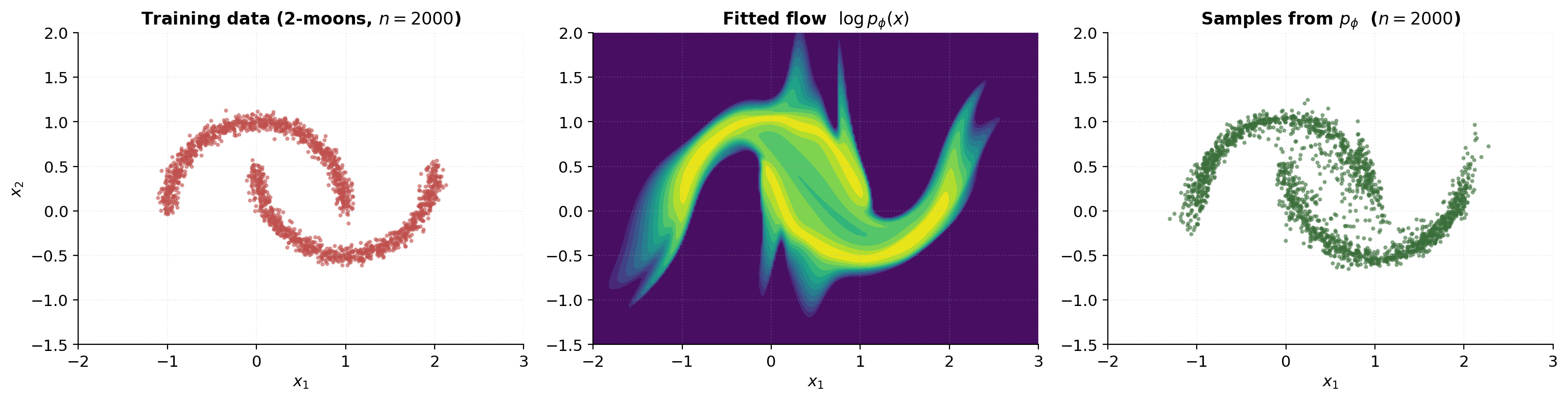
Worked example: 2-moons end-to-end
This is the synthesis section. Everything we’ve built up — the change-of-variables formula, the coupling-layer architecture, the MLE training recipe, the diagnostic suite — comes together to fit a 6-layer affine-coupling RealNVP to the canonical 2-moons dataset. No new math, no new architecture. Just the load-bearing machinery from §4 and §7 applied to a target that’s structurally harder than the §7 bimodal toy.
Dataset and base distribution
The 2-moons dataset (sklearn.datasets.make_moons) is the canonical 2-D toy for nonlinear separability — two interlocking crescent shapes that no axis-aligned linear classifier can separate. For density estimation we treat it as unsupervised: the binary class label is discarded, and the flow has to fit the joint distribution of over the union of both crescents.
We use samples with Gaussian noise of added to each point. The resulting cloud occupies roughly and , with the two crescents centered near and .
Why 2-moons is harder than the §7 bimodal target. The §7 target was two well-separated Gaussian blobs sharing the same axis — a single coupling layer with mask (“pass through, transform conditioned on ”) could split the blobs into the two halves and adjust independently for each. The 2-moons crescents intertwine: at any vertical slice with , both crescents have points at different values, and a single dimension partition cannot isolate one crescent from the other. The flow has to bend smoothly to wrap each crescent — exactly the kind of architectural test the §4 alternating-mask coupling stack is designed for.
The base distribution stays . The flow’s job is to find a diffeomorphism that pushes this isotropic Gaussian into the 2-moons-shaped target.
Six-layer RealNVP architecture and training
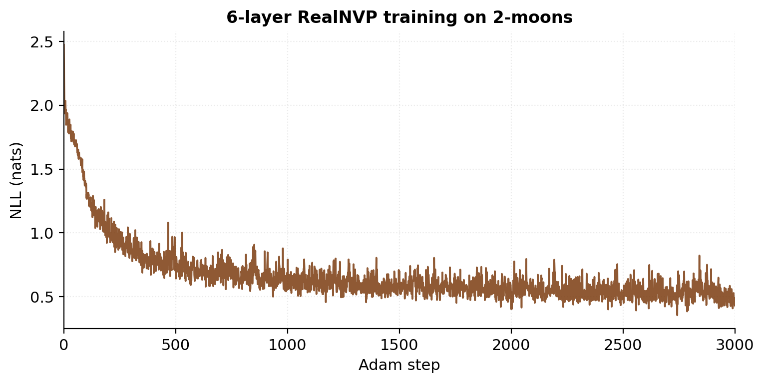
The architecture is CouplingFlow(d=2, n_layers=6, hidden=64) — six affine-coupling layers with alternating masks and a 64-unit trunk per layer. Compared to §7’s 4-layer hidden=32 flow we add two more layers and double the hidden width, reflecting the harder target.
Training: Adam at learning rate , batch size 256, 3000 steps. Total runtime: roughly 25 seconds on a 2020-era CPU. The training NLL drops substantially over the first steps and continues to refine for the remaining 2000. Unlike §7’s bimodal target, 2-moons has no closed-form entropy, so the optimal NLL is unknown a priori; the converged value is the empirical achievable bound for this architecture.
Learned density heatmap and sample scatter
Three-panel comparison: the training data, the fitted-density heatmap, and a fresh batch of samples drawn from the trained flow.
The fitted density should match the training data’s spatial extent — high density on the two crescents, low density in the gap between them. The flow’s samples should look visually indistinguishable from the training data: same crescent shapes, same approximate density across the support, same noise level.
A few diagnostic things to look for in the fitted-density heatmap:
- The density should be highest along the crescent centers, falling off smoothly toward the edges.
- The gap between crescents should be visible but not perfectly empty — recall §8.3’s topological barrier — the flow has to assign some low but nonzero density to the bridge between modes because diffeomorphisms cannot make the support disconnected.
- The density should not extend far outside the training-data envelope — no “phantom” high-density regions away from the data. A flow that over-extrapolates is the signature of either insufficient training (loss hasn’t converged) or insufficient depth.
Forward and inverse maps visualized
The most informative single visualization of a trained flow is the forward-map deformation of a regular grid: take a uniform grid of horizontal and vertical lines in -space and push it through . The grid lines come out bent and curved, wrapping around the 2-moons shape — a visual record of how the flow stretches and compresses the latent space to fit the data.
Symmetrically, the inverse map shows the flow’s “normalizing” action: take the training data, pull each point back through , and plot the resulting latents in -space. They should form an isotropic Gaussian-looking cloud, with 1- and 2- reference rings showing the expected density envelope. The §7 latent-Gaussianity diagnostic applied to the 2-moons-trained flow gives a tighter QQ-fit than the bimodal case — the more capacity helps.
Together, the two panels are the geometric content of the flow: the forward map curves the simple base distribution into the complex target; the inverse map flattens the complex target into the simple base. The two are exact inverses of each other up to floating-point precision (the §4 round-trip assertions verified this), and the visualization shows both directions simultaneously.
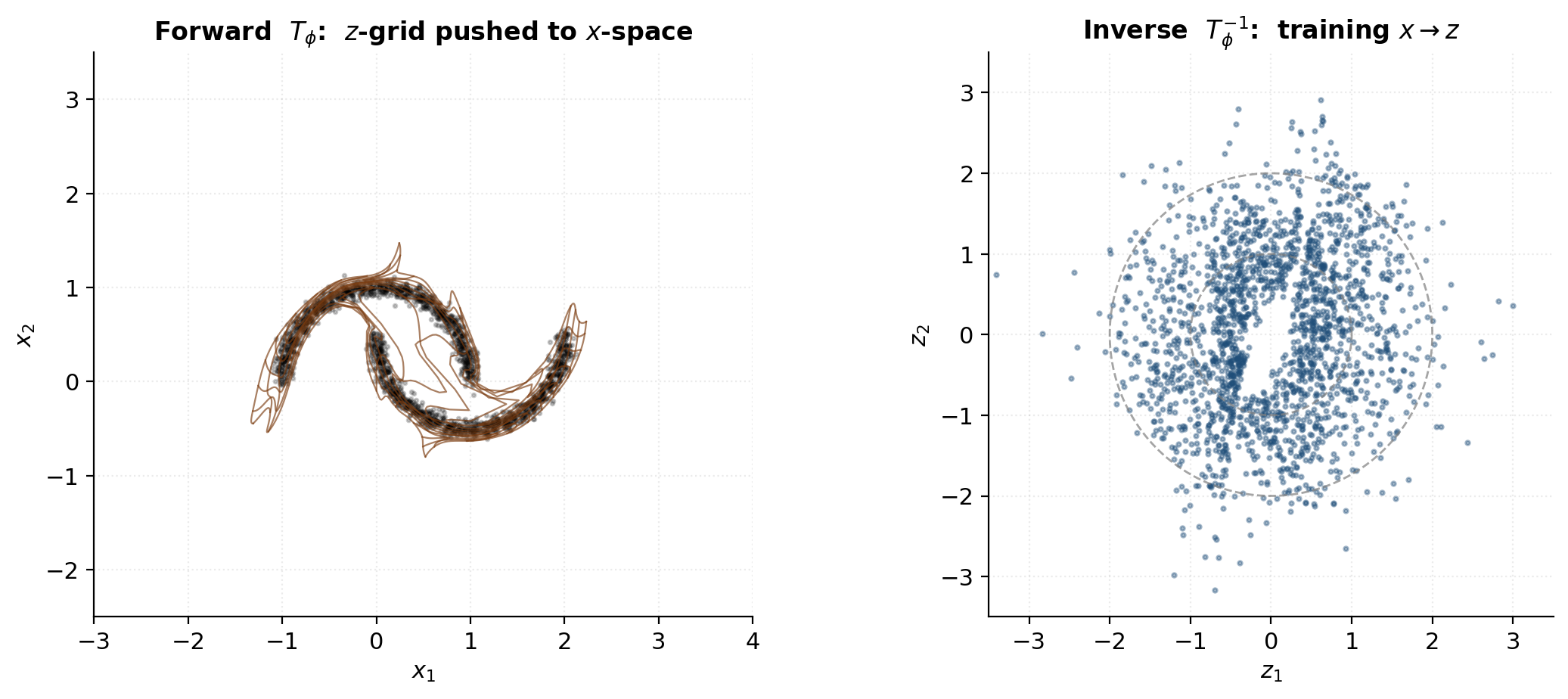
Connections, applications, and limits
This is the closing section. No new math, no new code — just the broader context. Where flows are used, what they cost, how they compare to other generative models, what they can’t do, and how they relate to sister-site topics on formalCalculus and formalStatistics.
Applications
Six application areas where flows do real work:
Image generation (Glow). Kingma and Dhariwal (2018) demonstrated that flows can scale to high-resolution image data with their multi-scale Glow architecture (§6). Glow trained on CelebA at 256 × 256 produces recognizable face images with smooth latent interpolations between samples. Subsequent work (RealNVP-FlowGAN hybrids, normalizing-flow-based super-resolution) has pushed image-domain flows further, though GANs and diffusion models still lead on raw sample quality (§12.4).
Molecular generation and Boltzmann sampling (equivariant flows). Köhler, Klein, and Noé (2020) and subsequent work introduced flows that respect 3-D rotational and translational equivariance, allowing them to sample molecular conformations from the Boltzmann distribution where is the potential energy. The equivariance constraint reduces the effective data dimensionality and makes the flow generalize across symmetric configurations without seeing them all during training. Application areas include drug-likeness scoring, free-energy estimation, and conformation sampling for molecular dynamics.
Reinforcement learning policy parameterization. Continuous-action RL (Mujoco environments, robotic control, motor-skill learning) typically parameterizes the policy as a Gaussian or mixture of Gaussians. Replacing this with an IAF gives much more flexible action distributions — capable of capturing multimodal optimal-action patterns that a Gaussian can’t. The use case is perfect for IAF (§5.3): sampling is cheap (we draw many actions per state during environment rollouts), and density evaluation on the model’s own samples is cheap (needed for the policy gradient and entropy-regularization terms). Mazoure, Doan, Durand, Pineau, and Hjelm (2020) is a representative entry point.
Simulation-based inference. For problems where the likelihood is intractable but we have a simulator producing given , flows amortize Bayesian inference by training on simulated pairs to learn the posterior directly. Methods like Sequential Neural Posterior Estimation (SNPE; Greenberg, Nonnenmacher, and Macke 2019) use flows as the conditional density estimator. Application areas: epidemiology (parameter estimation in compartment models), neuroscience (neural circuit models), cosmology (cosmological parameter inference). Cranmer, Brehmer, and Louppe (2020) survey the field.
Lossless compression. A trained flow gives exact , which via the Shannon–Fano–Elias scheme translates into a lossless compression rate of approximately bits per data point. Bits-Back coding (Ho, Lohn, Sutskever, and Abbeel 2019) achieves near-optimal rates on standard benchmarks. The catch: encoding and decoding must traverse the flow forward and backward respectively, which is much slower than fixed-codebook compressors.
Density-based out-of-distribution detection. A trained flow can in principle flag OOD samples by their low log-likelihood under . In practice this is more nuanced than it sounds: Nalisnick, Matsukawa, Teh, Görür, and Lakshminarayanan (2019) showed that flows trained on CIFAR-10 assign higher likelihood to SVHN images than to held-out CIFAR-10 images — a striking counterexample to the naive intuition that “OOD = low likelihood.” The community has converged on more sophisticated OOD scores (typicality tests, density ratios, likelihood-ratio statistics) rather than raw . This is an active research area.
Computational and memory profile
A flow’s cost has three regimes worth distinguishing.
Training step. A coupling-flow training step at depth , batch size , data dimension , hidden width costs roughly FLOPs for the forward pass (forward + inverse + log-det), plus a similar amount for the backward pass. For Glow-scale models at , , , : about FLOPs per training step, or roughly 1 second on a 2020-era GPU. Comparable to a VAE of similar capacity.
Memory. For exact gradient computation, the backward pass needs the forward activations of every coupling layer. At Glow scale, that’s roughly 12 MB per data point — manageable for batch size 32, but it grows linearly with batch size. Reversible-flow architectures (which coupling layers automatically are) admit a memory-saving trick: during the backward pass, recompute activations from later layers using invertibility rather than storing them. This trades compute for memory — useful for very deep stacks or large batches.
Sampling and density evaluation. Per data point: forward passes for sampling, inverse passes for density evaluation, both at the same cost as the training forward pass. For coupling flows, both directions cost the same; for autoregressive flows (§5), one direction is parallel ( MADE passes) and the other is sequential ( MADE passes). Glow-scale image generation at 256 × 256 takes roughly 100 ms per sample on a GPU — slow for real-time generation but fine for batch processing.
The asymptotic story: flows have constant per-data-point cost in both directions — no Markov chain sampling, no iterative inference. This is the source of flows’ practical sampling-speed advantage over diffusion models.
Flows vs VAEs vs GANs vs diffusion — trade-off table
A summary of the four major continuous-density generative-modeling families. The table reads as a capability matrix; the choice between them depends on which capabilities your application needs.
| Flow | VAE | GAN | Diffusion | |
|---|---|---|---|---|
| Training objective | Exact MLE | ELBO (lower bound) | Adversarial (min-max) | Score-matching / DDPM ELBO |
| Sampling cost | 1 forward pass ( layers) | 1 decoder pass | 1 generator pass | steps |
| Density evaluation | Exact | Lower bound (ELBO) | Unavailable | Lower bound or score estimate |
| Sample quality (images) | Moderate | Moderate (often blurry) | Excellent | Excellent |
| Mode coverage | Strong (mode-covering) | Strong (mode-covering) | Weak (mode collapse) | Strong |
| Latent-dim flexibility | Fixed = data dim | Free (bottleneck) | Free | Fixed = data dim |
| Implementation complexity | Moderate (arch constraints) | Low | High (adversarial, mode collapse) | Moderate (DDPM scheduling) |
| Invertibility | Yes (by design) | No | No | No |
| Likelihood ratios | Direct | Bounded | Discriminator estimate | Score difference |
A few patterns worth noticing:
- For exact density evaluation (likelihood-ratio tests, Bayesian model comparison, lossless compression, OOD detection), flows are the only family that gives an unbiased answer. VAE ELBOs are bounded, GAN densities are unavailable, diffusion ELBOs are bounded.
- For sample-quality-focused applications (image generation, audio synthesis), diffusion and GANs lead. Flows are typically a step behind on FID and Inception scores.
- For applications that need both directions cheaply (VI, RL policies, simulation-based inference), flows (specifically IAF and coupling) are the natural choice.
- For embedding into a probabilistic graphical model where the variational distribution needs to plug into an ELBO with exact entropy, flows are again the obvious choice (§9).
| Capability | Flow | VAE | GAN | Diffusion |
|---|---|---|---|---|
| Training objective | ||||
| Sampling cost | ||||
| Density evaluation | ||||
| Sample quality (images) | ||||
| Mode coverage | ||||
| Latent-dim flexibility | ||||
| Invertibility |
Honest limits
What flows can’t do well, or can only do at high cost:
High-dimensional expressivity bottleneck. Despite universality theorems (§8.1), flows in practice lag GANs and diffusion on high-resolution image quality. Glow-256 produces recognizable but artifact-laden samples; SOTA GANs (StyleGAN3) and diffusion models (Imagen, Stable Diffusion) produce photorealistic output. The structural reason is plausibly the effective receptive field: an affine-coupling layer can only directly correlate dimensions in the same mask partition, and alternating masks propagate correlations across depth in steps. For high-resolution images, layers don’t propagate enough cross-pixel correlation.
Training instability at very deep stacks. Very deep flow stacks () can be hard to train stably even with all the §7.3 stability tricks. Spline flows (§6.4) help by being more expressive per layer; continuous flows (§8.4) help by being effectively continuous-depth.
Sample-quality lag. Flows trained for density estimation often produce blurrier samples than GANs and diffusion. The mode-covering MLE objective (§7.1) prefers smooth interpolation between training points — it covers every region of the data but smooths across narrow features. For applications where sharp samples matter more than density correctness (game-engine asset generation, photoreal portraits), GANs and diffusion are the right tools.
Dimension-preservation cost. A flow on a -dim image has -dim latents — no bottleneck. A VAE on the same data uses or so. The flow uses way more parameters per data point (the networks model interactions across all dims) and may overfit small datasets accordingly. For tasks where the underlying data lies on a much lower-dimensional manifold, VAEs’ explicit bottleneck is a feature, not a bug.
OOD detection failure modes. The naive use of as an OOD score fails reliably enough to be a research embarrassment (Nalisnick et al. 2019; §12.1). The community has converged on more nuanced scores; flows remain useful for OOD detection, but not via the route the original Glow paper suggested.
Topological barrier (already §8.3). Diffeomorphisms preserve topology; flows can’t model genuinely discontinuous-support distributions cleanly. For data with discrete component structure (categorical mixtures, isolated submanifolds), other architectures (mixture models, hybrid VAEs with categorical latents) are structurally better.
Computational cost relative to diffusion. While flows are faster than diffusion at sampling time (1 forward pass vs 100–1000 denoising steps), they’re slower at training time for equivalent sample quality on high-resolution data. Diffusion’s denoising-network parameterization is highly parameter-efficient relative to a coupling stack, so a diffusion model with the same training budget reaches better sample quality. The trade-off: pay at training time (diffusion) or at sampling time (flow).
Cross-site topology
The relationships to sister-site topics, summarized:
formalCalculus prereqs. Two load-bearing topics: formalCalculus: Change of Variables (the substitution rule for densities — the entire framework is downstream of it; derived in §2.2) and formalCalculus: Jacobian (the determinant of the Jacobian as a volume-distortion factor — the architectural design pressure for triangular Jacobians, §4). For readers who need to refresh either, the formalCalculus topics are the recommended starting points.
formalStatistics prereqs. Three connections worth naming:
- formalStatistics: Kernel Density Estimation — the nonparametric predecessor that flows generalize to a neural-parametric form. §10.2 details the contrast: KDE wins at low and small , flows win at high and large . The two are complementary tools, not competitors.
- formalStatistics: Maximum Likelihood — the training objective in §7 is plain MLE applied to a flow’s parametric family. The consistency, asymptotic efficiency, and bias-variance trade-off all inherit from classical MLE theory.
- formalStatistics: Multivariate Distributions — the standard multivariate Gaussian as the base, the multivariate change-of-variables for the pushforward, and the joint–marginal–conditional decomposition for the autoregressive form (§5).
formalML connections. Two:
- Variational Inference — §9 is the bridge. Flows are flexible variational families that strictly improve over Gaussian mean-field VI when the posterior is non-Gaussian. The flow-VI ELBO derivation and the sign-flip arithmetic live in §9.3.
- Density Ratio Estimation (coming soon) — for problems where is needed rather than . §10.4 forward-points; the shared neural-parametric methodology makes the two topics natural companions.
The diffusion successor. Score-based generative models and denoising diffusion (Sohl-Dickstein, Weiss, Maheswaranathan, and Ganguli 2015; Ho, Jain, and Abbeel 2020; Song and Ermon 2019) are the architectural successor to flows for sample-quality-focused applications. They sacrifice the exact density (replaced by a score-matching or DDPM-ELBO objective) for dramatically better sample quality at high resolution. Diffusion is its own topic; this topic forward-points but doesn’t derive. Readers who hit the expressivity wall of discrete coupling flows for image-domain applications should look there next.
This concludes the topic. The §11 worked example is the canonical artifact; the §4 and §5 architectures are the load-bearing implementations; the §7 training recipe is the engineering workflow. The rest is context.
Connections
- §9 is the bridge: flows can serve as flexible variational families that strictly improve over Gaussian mean-field VI when the posterior is curved, multimodal, or heavy-tailed. The flow-VI ELBO derivation in §9.3 reuses the change-of-variables formula from §2 with the entropy sign-flip — same machinery, opposite sign in front of the log-det. Rezende and Mohamed's 2015 paper that coined 'normalizing flow' is a VI paper, not a density-estimation paper. variational-inference
- Both topics use neural networks to parameterize probability distributions, but with different architectural pressure. BNNs put a prior on the network weights and approximate the posterior (Laplace / MC dropout / SG-MCMC / deep ensembles); flows fix the weights deterministically and put structure on the function the network represents (an invertible map). The two are complementary tools — a Bayesian neural flow is a flow with a posterior over its weights. bayesian-neural-networks
- Both topics confront the high-$d$ regime, but the structural pressure differs. High-dim regression uses sparsity (lasso) or low-rank structure (PCA) to identify a low-dimensional signal subspace; flows preserve full dimensionality and use the triangular-Jacobian trick to keep the log-det $O(d)$ instead of $O(d^3)$. The lasso's restricted-eigenvalue condition and the flow's triangular Jacobian are both architectural devices for taming high-dimensional joint distributions. high-dimensional-regression
References & Further Reading
- paper Density Estimation by Dual Ascent of the Log-Likelihood — Tabak & Vanden-Eijnden (2010) Communications in Mathematical Sciences. The pre-deep-learning origin of cascaded-diffeomorphism density estimation.
- paper A Family of Nonparametric Density Estimation Algorithms — Tabak & Turner (2013) Communications on Pure and Applied Mathematics. Continues the §3.4 historical line — flows as cascaded invertible maps in applied math.
- paper Variational Inference with Normalizing Flows — Rezende & Mohamed (2015) ICML. The paper that coined the name and brought flows into deep learning; the VI use case in §9.
- paper NICE: Non-linear Independent Components Estimation — Dinh, Krueger & Bengio (2015) ICLR workshop. Additive coupling — the volume-preserving precursor to RealNVP (§4.2).
- paper Density Estimation Using Real NVP — Dinh, Sohl-Dickstein & Bengio (2017) ICLR. Affine coupling — the load-bearing architecture for §4 and §11's worked example.
- paper Glow: Generative Flow with Invertible 1x1 Convolutions — Kingma & Dhariwal (2018) NeurIPS. Multi-scale architecture, 1×1 invertible convolutions, and ActNorm — the §6 primitives.
- paper MADE: Masked Autoencoder for Distribution Estimation — Germain, Gregor, Murray & Larochelle (2015) ICML. The masked-autoencoder substrate MAF and IAF condition through (§5).
- paper Masked Autoregressive Flow for Density Estimation — Papamakarios, Pavlakou & Murray (2017) NeurIPS. MAF — parallel density evaluation, sequential sampling (§5.2).
- paper Improving Variational Inference with Inverse Autoregressive Flow — Kingma, Salimans, Jozefowicz, Chen, Sutskever & Welling (2016) NeurIPS. IAF — the MAF-dual built for VI use cases (§5.3, §9.4).
- paper Neural Spline Flows — Durkan, Bekasov, Murray & Papamakarios (2019) NeurIPS. Rational-quadratic monotone update inside coupling layers — §6.4's expressivity sweet spot.
- paper Neural Ordinary Differential Equations — Chen, Rubanova, Bettencourt & Duvenaud (2018) NeurIPS. Continuous-time flow precursor — §8.4's instantaneous change-of-variables formula.
- paper FFJORD: Free-form Continuous Dynamics for Scalable Reversible Generative Models — Grathwohl, Chen, Bettencourt, Sutskever & Duvenaud (2019) ICLR. Hutchinson trace trick brings continuous-flow log-det to $O(d)$ stochastically (§8.4).
- paper Coupling-Based Invertible Neural Networks Are Universal Diffeomorphism Approximators — Teshima, Ishikawa, Tojo, Oono, Ikeda & Sugiyama (2020) NeurIPS. Universality theorem for affine-coupling flows in §8.1.
- paper Normalizing Flows for Probabilistic Modeling and Inference — Papamakarios, Nalisnick, Rezende, Mohamed & Lakshminarayanan (2021) JMLR. The standard survey — comprehensive framework treatment.
- paper Normalizing Flows: An Introduction and Review of Current Methods — Kobyzev, Prince & Brubaker (2021) IEEE TPAMI. Complementary survey to Papamakarios et al. (2021).
- paper Equivariant Flows: Exact Likelihood Generative Learning for Symmetric Densities — Köhler, Klein & Noé (2020) ICML. Rotation/translation-equivariant flows for molecular Boltzmann sampling (§12.1).
- paper The Frontier of Simulation-Based Inference — Cranmer, Brehmer & Louppe (2020) PNAS. Survey of simulation-based inference — flows as the conditional density estimator (§12.1).
- paper Automatic Posterior Transformation for Likelihood-Free Inference — Greenberg, Nonnenmacher & Macke (2019) ICML. SNPE algorithm — flows as the amortized posterior density estimator (§12.1).
- paper Do Deep Generative Models Know What They Don't Know? — Nalisnick, Matsukawa, Teh, Gorur & Lakshminarayanan (2019) ICLR. The CIFAR-vs-SVHN OOD-counterexample paper (§12.1, §12.4).
- paper Leveraging Exploration in Off-Policy Algorithms via Normalizing Flows — Mazoure, Doan, Durand, Pineau & Hjelm (2020) CoRL. RL policy parameterization with IAF — the §12.1 RL application.
- paper Deep Unsupervised Learning using Nonequilibrium Thermodynamics — Sohl-Dickstein, Weiss, Maheswaranathan & Ganguli (2015) ICML. The original diffusion-model paper — the architectural successor to flows (§12.5).
- paper Denoising Diffusion Probabilistic Models — Ho, Jain & Abbeel (2020) NeurIPS. DDPM — the canonical modern diffusion model that flows forward-point to in §12.5.
- paper Generative Modeling by Estimating Gradients of the Data Distribution — Song & Ermon (2019) NeurIPS. Score-based generative modeling — diffusion's gradient-of-log-density formulation (§12.5).