High-Dimensional Regression

§1. From OLS to penalized regression

When the predictor matrix has more columns than rows, ordinary least squares stops being a single estimator and becomes a degenerate family — infinitely many vectors fit the training data perfectly, none of them generalize. This section establishes the high-dimensional regime, shows OLS failing on the canonical sparse-Gaussian-design problem we’ll reuse for the next eight sections, and introduces the two classical regularization remedies: ridge (L2-penalized) and lasso (L1-penalized). Ridge gives a unique solution and shrinks every coefficient smoothly toward zero; lasso gives a sparse solution and shrinks small coefficients all the way to zero. The geometric difference between those two penalties — corners on the L1 ball, smooth curvature on the L2 ball — is what makes the lasso the central object of this topic.

§1.1 The high-dimensional regime $p \gtrsim n$ and where it appears

Standard regression theory assumes more observations than features ($n > p$), often by orders of magnitude. The high-dimensional regime flips that: $p$ is comparable to or much larger than $n$. Three places it shows up routinely:

• Genome-wide association studies (GWAS). Regress a phenotype on hundreds of thousands to millions of single-nucleotide polymorphisms. Typical scale is $p \approx 10^6$ with $n \approx 10^4$ patients; the ratio $p / n \approx 100$ is normal, not extreme.
• Functional MRI. A whole-brain scan resolves $\sim 10^5$ voxels per timepoint; predicting a behavioral or clinical outcome from voxel-level activations gives $p \approx 10^5$ with $n$ in the low hundreds.
• Text and high-cardinality categorical features. A bag-of-words encoding of even a modest corpus pushes $p$ into the millions while $n$ stays in the thousands.

These problems share more than $p \gg n$ — they also tend to be sparse: only a small subset of features carries the actual signal. A handful of SNPs drive most of the heritable variation in a quantitative trait; a focal brain region carries most of the predictive signal in an fMRI study; a few keywords carry most of the topic information in a document. The lasso’s design exploits this sparsity directly.

We’ll formalize sparsity as $\|\boldsymbol\beta^*\|_0 = s$ where $s \ll p$ — the true coefficient vector $\boldsymbol\beta^* \in \mathbb{R}^p$ has only $s$ nonzero entries. The set $S = \{j : \beta^*_j \neq 0\}$ is the support of $\boldsymbol\beta^*$, and $|S| = s$ is the sparsity level. We don’t know $S$ in advance; recovering it (or, more modestly, predicting well without recovering it) is the estimator’s job.

The canonical sparse high-dimensional dataset (DGP-1). We’ll reuse the same data-generating process across §§2–9 to make the comparisons concrete. Fix:

• $n = 200$, $p = 500$, $s = 10$.
• Rows $\mathbf{x}_i \in \mathbb{R}^p$ iid $\mathcal{N}(\mathbf{0}, \boldsymbol\Sigma)$ with $\boldsymbol\Sigma_{jk} = 0.5^{|j-k|}$ (AR(1) Toeplitz, weakly decaying off-diagonal correlation).
• $\beta^*_j = 1$ for $j \in S = \{0, 1, \dots, 9\}$ (contiguous active set), $\beta^*_j = 0$ otherwise.
• Noise $\boldsymbol\varepsilon \sim \mathcal{N}(\mathbf{0}, \sigma^2 \mathbf{I})$ with $\sigma = 0.5$.
• Population $R^2 \approx 0.99$ (computed: $\boldsymbol\beta^{*\top} \boldsymbol\Sigma \boldsymbol\beta^* \approx 26.0$ via the AR(1) sum over a 10×10 active block).
• Seed: np.random.default_rng(42).

The §10 debiased-lasso coverage demonstration switches to $(n, p, s) = (200, 100, 5)$ to make OLS feasible as a baseline. All other sections reuse DGP-1.

§1.2 Why OLS fails: the rank-deficient normal equations

OLS minimizes the squared training loss:

$$\hat{\boldsymbol\beta}^{\text{OLS}} = \arg\min_{\boldsymbol\beta \in \mathbb{R}^p} \frac{1}{n} \|\mathbf{y} - \mathbf{X} \boldsymbol\beta\|_2^2,$$

with the closed-form solution $\hat{\boldsymbol\beta}^{\text{OLS}} = (\mathbf{X}^\top \mathbf{X})^{-1} \mathbf{X}^\top \mathbf{y}$ when $\mathbf{X}^\top \mathbf{X}$ is invertible. Invertibility requires $\text{rank}(\mathbf{X}) = p$, which in turn requires $n \ge p$.

When $p > n$, the matrix $\mathbf{X}^\top \mathbf{X} \in \mathbb{R}^{p \times p}$ has rank at most $n < p$ and is singular. The normal equations $\mathbf{X}^\top \mathbf{X} \boldsymbol\beta = \mathbf{X}^\top \mathbf{y}$ have infinitely many solutions: for any vector $\mathbf{v}$ in the $(p - n)$-dimensional null space of $\mathbf{X}$, both $\hat{\boldsymbol\beta}$ and $\hat{\boldsymbol\beta} + \mathbf{v}$ achieve the same residual. The OLS objective has a flat plateau of global minima, all of them interpolating the training data exactly.

The standard pseudoinverse fix picks the minimum-norm solution from that plateau:

$$\hat{\boldsymbol\beta}^{\text{OLS, min-norm}} = \mathbf{X}^\top (\mathbf{X} \mathbf{X}^\top)^{-1} \mathbf{y},$$

well-defined whenever $\mathbf{X}$ has full row rank. But “minimum-norm OLS” is still OLS — it interpolates the training data ($\mathbf{X} \hat{\boldsymbol\beta} = \mathbf{y}$), the training MSE is exactly zero, and the test MSE is unbounded. Even before $p$ reaches $n$, predictive performance degrades: as $p \to n$ from below, the smallest singular value of $\mathbf{X}$ approaches zero, $(\mathbf{X}^\top \mathbf{X})^{-1}$ blows up, and the OLS coefficient estimates inflate even though the in-sample fit looks great.

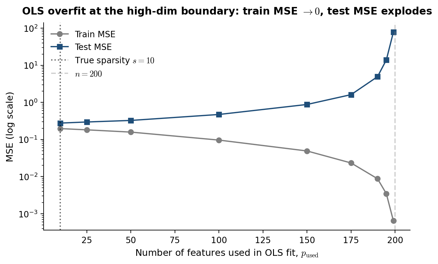
Sweep the active feature count from $p_{\text{used}} = 10$ to $p_{\text{used}} = 199$ on a fresh DGP-1 sample, fit OLS to each subproblem (using only the first $p_{\text{used}}$ columns of $\mathbf{X}$), and plot train MSE and test MSE on log-y. Train MSE drops monotonically toward zero as $p_{\text{used}}$ approaches $n$. Test MSE bottoms out near $p_{\text{used}} \approx s = 10$ (the truth) and explodes by orders of magnitude as $p_{\text{used}} \to n$. The reader sees, in one picture, that OLS is incapable of using the sparsity structure — it doesn’t know that only 10 features matter, so it overfits aggressively as soon as it has the degrees of freedom to do so.

OLS on DGP-1 (n = 200, σ = 0.5, AR(1) ρ = 0.5, s = 10). Train MSE drops to zero as p_used → n; test MSE bottoms near p_used = s and explodes near the rank-deficiency boundary p_used = n. Hover any point for exact values. Computed live in-browser with Cholesky-based ridge OLS (jitter ε = 1e-8 for numerical stability at large p_used).

§1.3 Ridge regression as the L2 fix

Ridge regression resolves the rank-deficiency by adding a quadratic penalty:

$$\hat{\boldsymbol\beta}^{\text{ridge}}(\lambda) = \arg\min_{\boldsymbol\beta \in \mathbb{R}^p} \frac{1}{2n} \|\mathbf{y} - \mathbf{X} \boldsymbol\beta\|_2^2 + \frac{\lambda}{2} \|\boldsymbol\beta\|_2^2,$$

where $\|\boldsymbol\beta\|_2^2 = \sum_{j=1}^p \beta_j^2$ is the squared L2 norm and $\lambda \ge 0$ is a tuning parameter ($\lambda = 0$ recovers OLS, $\lambda \to \infty$ shrinks every coefficient to zero). The closed form is:

$$\hat{\boldsymbol\beta}^{\text{ridge}}(\lambda) = (\mathbf{X}^\top \mathbf{X} + n \lambda \mathbf{I})^{-1} \mathbf{X}^\top \mathbf{y}.$$

The matrix $\mathbf{X}^\top \mathbf{X} + n\lambda \mathbf{I}$ is positive definite for any $\lambda > 0$ — its eigenvalues are bounded below by $n\lambda$ — so the inversion is well-defined regardless of whether $p \le n$ or $p > n$. Ridge restores uniqueness.

Two structural properties matter for what follows:

1. Continuous shrinkage, dense solutions. Each coefficient is shrunk toward zero by a factor that depends on the corresponding singular value of $\mathbf{X}$, but no coefficient is set to exactly zero (with probability one over a continuous design). On DGP-1, ridge produces 500 nonzero coefficients even though only 10 features matter.
2. Smoothness in $\lambda$. $\hat{\boldsymbol\beta}^{\text{ridge}}(\lambda)$ is a continuous, differentiable function of $\lambda$ everywhere on $[0, \infty)$. There’s no “selection event” — coefficients shrink, they don’t snap.

Ridge is the right tool when all features carry some signal and the goal is to stabilize coefficient estimates against multicollinearity. In the high-dimensional sparse regime where the truth has 10 active features out of 500, ridge’s refusal to zero out the 490 inactive features is a liability — every irrelevant coefficient contributes variance to the prediction. The standard formalstatistics treatment of ridge covers the $n > p$ case and the Bayesian Gaussian-prior interpretation; we’re using ridge here as the dense-shrinkage baseline that lasso will improve on.

§1.4 The lasso as the L1 alternative

The lasso (Tibshirani 1996) replaces the squared L2 penalty with an L1 penalty:

$$\hat{\boldsymbol\beta}^{\text{lasso}}(\lambda) = \arg\min_{\boldsymbol\beta \in \mathbb{R}^p} \frac{1}{2n} \|\mathbf{y} - \mathbf{X} \boldsymbol\beta\|_2^2 + \lambda \|\boldsymbol\beta\|_1,$$

where $\|\boldsymbol\beta\|_1 = \sum_{j=1}^p |\beta_j|$ is the L1 norm. The objective is convex (squared loss is convex, L1 norm is convex, sum of convex is convex), so any local minimum is a global minimum. But the L1 norm is not differentiable at zero, and that non-smoothness has two consequences that turn out to be central:

1. Sparsity. The optimal solution has many coefficients exactly equal to zero, and the number of nonzero coefficients is controlled by $\lambda$. Geometrically, the L1 ball $\{\boldsymbol\beta : \|\boldsymbol\beta\|_1 \le t\}$ has corners at the coordinate axes; the constrained-form lasso solution is the point where the squared-loss contour first touches the L1 ball as the ball expands, and that contact point is generically at a corner — i.e., on a coordinate hyperplane, with one or more coefficients zero. The smooth L2 ball has no corners, which is why ridge solutions are dense. We’ll come back to this picture in §2.2 with an interactive viz.
2. No closed form in general. Unlike ridge, the lasso has no general closed-form solution. There is one when the design is orthogonal ($\mathbf{X}^\top \mathbf{X} = n \mathbf{I}$, derived in §3.1 via the soft-thresholding operator), but for general $\mathbf{X}$ the solution requires an iterative solver. §3 covers coordinate descent, ISTA, and FISTA in detail.

The L1 penalty is the smallest convex penalty that produces sparsity. The non-convex L0 penalty $\|\boldsymbol\beta\|_0 = |\{j : \beta_j \neq 0\}|$ would also produce sparse solutions — and is in some ways the “right” objective for variable selection — but the resulting optimization problem is best-subset selection, which is NP-hard. The L1 penalty is the convex relaxation of L0: among convex penalties that produce sparsity, it’s the simplest to state, the easiest to optimize, and the one with the best-developed statistical theory.

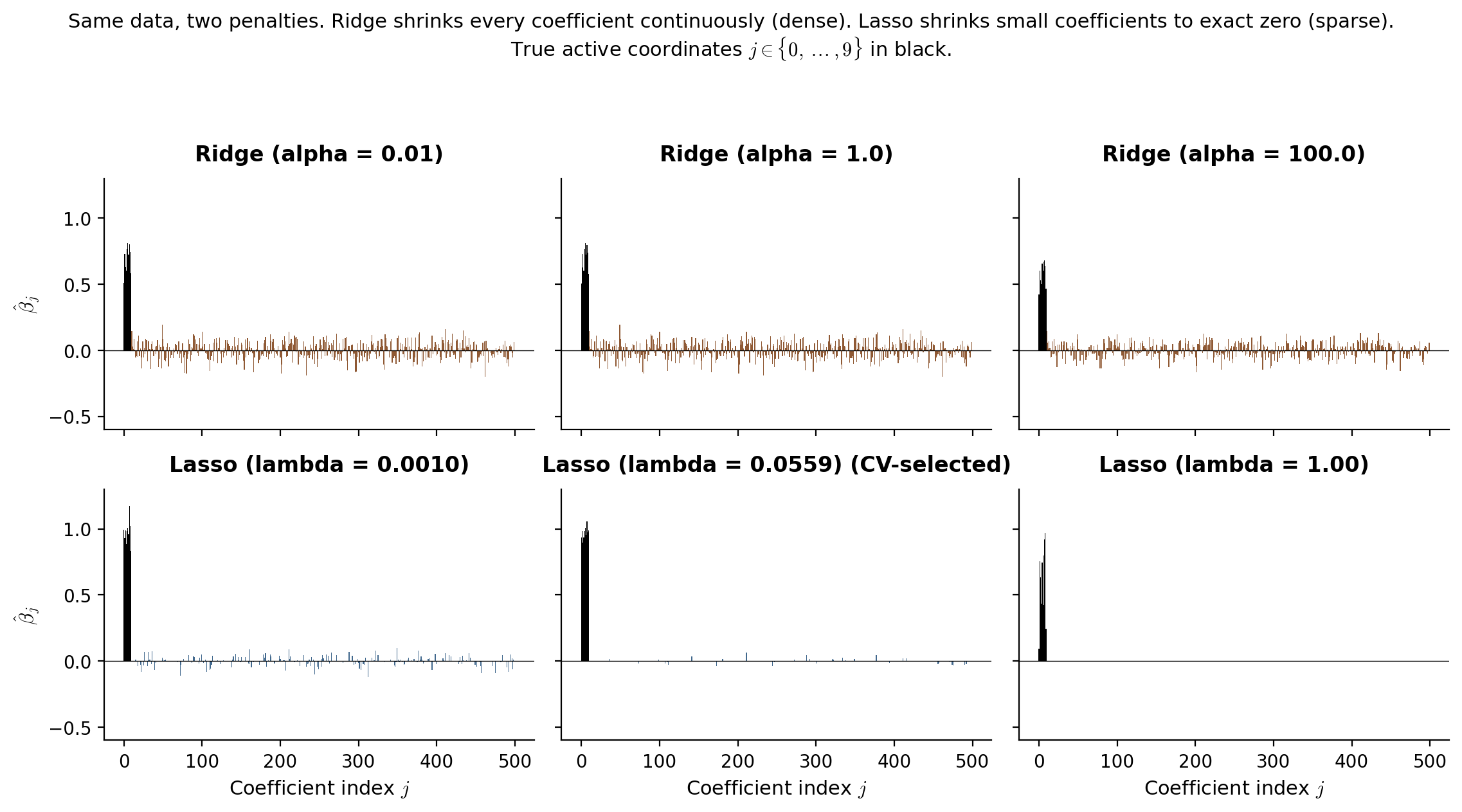
Side-by-side: ridge at three penalty levels ($\alpha \in \{0.01, 1, 100\}$) and lasso at three penalty levels ($\lambda \in \{0.001, \lambda_{\text{CV}} \approx 0.056, 1\}$), all on the same DGP-1 sample. Ridge produces 500 nonzero coefficients at every $\alpha$ — heavier penalization means smaller coefficients across the board, never exactly zero. The lasso at the CV-selected $\lambda$ has only ~12 nonzero coefficients, mostly concentrated at the true active coordinates $S = \{0, \dots, 9\}$. The contrast is the visual punchline of the section.

Ridge (top row, three α levels) vs lasso (bottom row, three λ levels) on DGP-1 (n = 200, p = 500, s = 10, σ = 0.5). True active coordinates (j < 10) in black; 490 inactive coordinates in gray. Ridge is dense at every α; lasso at the CV-selected λ ≈ 0.056 produces a sparse fit concentrated at the true active set. Computed live in-browser via Cholesky-based ridge with pre-computed XᵀX (shared across α levels) and 200-iteration ISTA for lasso. Compute ~1 second; viz is hidden until scrolled into view.

§1.5 Roadmap

The rest of the topic answers four questions about the lasso. What does the estimator look like? §2 fills in the geometric picture and basic structural results — existence, uniqueness, KKT subgradient conditions. How do we compute it? §3 derives the soft-thresholding closed form for orthogonal designs and develops the iterative solvers (coordinate descent, ISTA, FISTA) used in general. Does it predict well, and does it recover the true support? §§4–6 work out the bias-variance trade-off, prove the headline non-asymptotic prediction-risk bound (the lasso oracle inequality, $O(\sigma^2 s \log p / n)$ under the restricted-eigenvalue condition), and treat variable-selection consistency as a separate theorem with its own sufficient condition (irrepresentable). §7 covers practical $\lambda$ selection by cross-validation and information criteria. §8 covers the ridge / elastic-net / adaptive-lasso variants and when each wins. §9 deepens the geometry of the high-dimensional regime — RIP, sub-Gaussian designs, the implication chain between conditions. Can we do inference with it? §10 is the inferential payoff: naive lasso confidence intervals undercover (PoSI; Berk et al. 2013), and the debiased-lasso construction (Zhang-Zhang 2014; Javanmard-Montanari 2014; van de Geer et al. 2014) restores valid coverage. §11 extends the lasso to non-Gaussian responses (logistic, Poisson). §12 closes with connections to double/debiased ML, causal inference, and the Bayesian counterpart in Sparse Bayesian Priors.

§2. The lasso estimator

The lasso is convex L1-penalized least squares — a well-defined, well-studied estimator with a clean geometric story and a precise first-order characterization. This section establishes the formal definition (in both penalized and constrained forms), develops the geometric intuition for why L1 penalization produces sparse solutions (corners on the L1 ball, smooth curvature on the L2 ball), addresses existence and uniqueness (Tibshirani 2013), and works out the KKT subgradient conditions that characterize every lasso solution. The KKT conditions are the load-bearing technical machinery for the rest of the topic — the soft-thresholding closed form in §3.1, the basic inequality in the oracle inequality proof of §5.2, and the debiased-lasso construction of §10.2 all derive from them.

§2.1 The L1-penalized least-squares definition

The lasso estimator is the minimizer of an L1-penalized squared loss:

Three things to note about the definition.

The $1 / (2n)$ scaling. The factor of $1/2$ in front of the squared loss is a convention that makes the gradient equal $-\mathbf{X}^\top (\mathbf{y} - \mathbf{X} \boldsymbol\beta) / n$ (no leading 2), and the $1/n$ normalization makes the objective an empirical average. With this scaling, $\lambda$ has units of “covariate-response correlation” — comparable across sample sizes — and the optimal $\lambda$ scales as $\sigma \sqrt{\log(p) / n}$ (we’ll see this in §5). The scikit-learn convention (and the one we’ll use throughout the notebook) matches: Lasso(alpha=λ) minimizes $\frac{1}{2n} \|\mathbf{y} - \mathbf{X} \boldsymbol\beta\|_2^2 + \alpha \|\boldsymbol\beta\|_1$, with the same $1/2n$ out front.

Convexity. The squared loss is strongly convex in $\mathbf{X} \boldsymbol\beta$ but only weakly convex in $\boldsymbol\beta$ when $\mathbf{X}$ has rank $< p$. The L1 norm is convex (every norm is), so the sum is convex. There are no local minima that aren’t global minima; the solution set is always a convex set in $\mathbb{R}^p$.

The L1 norm is not differentiable at zero. $|\beta_j|$ is differentiable everywhere except $\beta_j = 0$, where the subgradient is the closed interval $[-1, 1]$. This non-smoothness is exactly what produces sparsity — and is also why the lasso has no closed-form solution in general (subgradients require a discrete case analysis at each coordinate).

Constrained-form duality. The penalized lasso is equivalent to the constrained-form lasso

$$\hat{\boldsymbol\beta}^{\text{lasso}}(t) = \arg\min_{\|\boldsymbol\beta\|_1 \le t} \frac{1}{2n} \|\mathbf{y} - \mathbf{X} \boldsymbol\beta\|_2^2,$$

via Lagrangian duality. For each $\lambda \ge 0$ there’s a corresponding budget $t(\lambda) = \|\hat{\boldsymbol\beta}^{\text{lasso}}(\lambda)\|_1$, and conversely each $t \in [0, \|\hat{\boldsymbol\beta}^{\text{OLS}}\|_1]$ corresponds to a unique $\lambda(t) \ge 0$. The mapping $t \leftrightarrow \lambda$ is monotone but not generally available in closed form. Both forms appear in the literature; the penalized form is more convenient for proofs (one term in the gradient, no constraint qualification needed), and the constrained form is more convenient for the geometric pictures we’ll draw next.

§2.2 Geometric picture: $L^1$ corners produce sparsity

Why does L1 penalization produce solutions with exact zeros? The cleanest answer is geometric: the L1 ball has corners on the coordinate axes, and the loss contour generically touches the ball at one of those corners.

Consider the constrained lasso in 2D with a fixed budget $t$. The feasible region $\{\boldsymbol\beta : \|\boldsymbol\beta\|_1 \le t\}$ is a diamond — a square rotated 45 degrees — with vertices at $(\pm t, 0)$ and $(0, \pm t)$. The objective contours $\{\boldsymbol\beta : \|\mathbf{y} - \mathbf{X} \boldsymbol\beta\|_2^2 = c\}$ are concentric ellipses centered at $\hat{\boldsymbol\beta}^{\text{OLS}}$ with axes determined by the eigenvectors of $\mathbf{X}^\top \mathbf{X}$. The constrained solution is the point where the smallest ellipse just touches the diamond.

If $\hat{\boldsymbol\beta}^{\text{OLS}}$ lies outside the diamond — which is the interesting case; otherwise the constraint is inactive — the contact point is on the diamond’s boundary. The boundary consists of four edges and four vertices. Generically, for almost every $\mathbf{X}^\top \mathbf{X}$ and $\hat{\boldsymbol\beta}^{\text{OLS}}$, the contact is at a vertex, not a smooth point on an edge. At a vertex, one coordinate is exactly zero. Sparsity.

The L2 ball is the disk $\{\boldsymbol\beta : \|\boldsymbol\beta\|_2 \le t\}$ — smooth, no corners. The contact point with an ellipse is generically a smooth point on the disk’s boundary, with both coordinates nonzero. Density.

This picture extends to $\mathbb{R}^p$ with $p > 2$. The L1 ball has $2p$ vertices (one per coordinate-axis intersection), $p(p-1)$ edges, and a hierarchy of lower-dimensional faces; contact at a $k$-dimensional face means the solution has exactly $p - k$ nonzero coordinates. The L2 ball has no faces of any positive codimension; contact is always smooth, the solution is always dense.

budget t = 1.00(release to recompute contacts)

β̂_OLS = (0.4, 1.6); Hessian H = [[1, 0.4], [0.4, 1]]; loss Q(β) = (β − β̂_OLS)ᵀ H (β − β̂_OLS). The amber dashed ellipse is the just-tangent loss contour at the L1 contact. As you drag t, watch the L1 contact stay pinned to the diamond's nearest vertex (one coordinate exactly zero) while the L2 contact slides smoothly around the disk. The L1 vertex generically achieves a lower loss than any edge interior — that's the geometric source of sparsity.

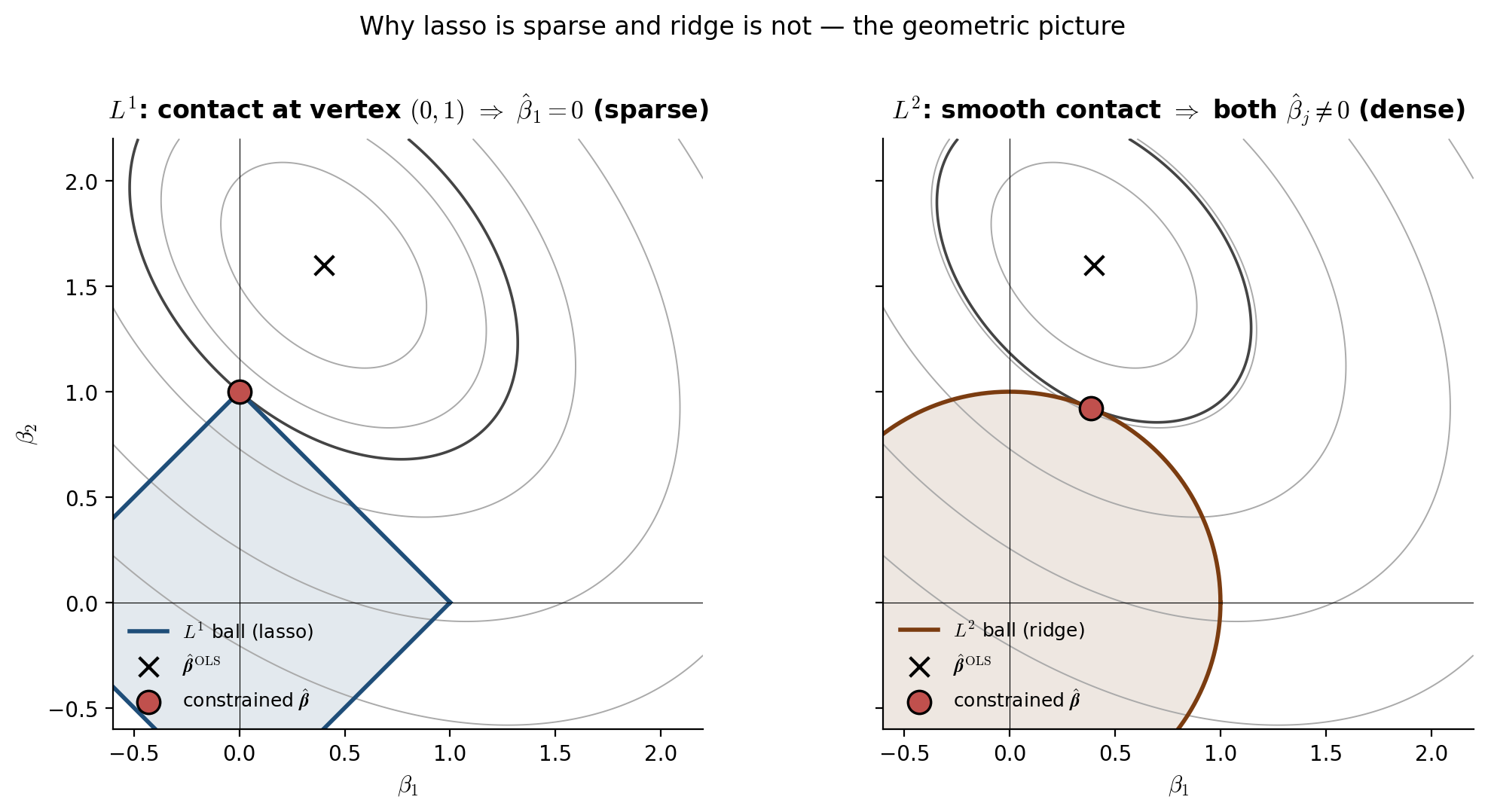
The figure is the geometric content of the lasso. Everything else — the soft-thresholding closed form (§3.1), the lasso path (§4.4), the active-set / equicorrelation-set characterization (§2.4 below) — is algebraic machinery that operationalizes it.

§2.3 Existence and uniqueness

Existence. The lasso objective is convex, continuous, and coercive — as $\|\boldsymbol\beta\| \to \infty$, the squared loss is bounded below by zero and the L1 penalty grows linearly, so the objective grows without bound. Convex-and-coercive implies attainment of the minimum, so the solution set $\hat{B}(\lambda) = \arg\min_{\boldsymbol\beta} \{(1/2n) \|\mathbf{y} - \mathbf{X} \boldsymbol\beta\|_2^2 + \lambda \|\boldsymbol\beta\|_1\}$ is non-empty for every $\lambda \ge 0$. The solution set is also convex (intersection of all minima of a convex function) and closed (by continuity).

Uniqueness. When does $\hat{B}(\lambda)$ contain a single point? Two sufficient conditions:

1. $p \le n$ and $\mathbf{X}$ has full column rank. Then $\mathbf{X}^\top \mathbf{X}$ is positive definite, the squared loss is strictly convex in $\boldsymbol\beta$, the lasso objective is strictly convex, and the minimum is unique.
2. $\mathbf{X}$ has columns in “general position”. Tibshirani (2013) showed that this condition — no $k+1$ columns of $\pm \mathbf{X}$ lie in an affine subspace of dimension $k - 1$ — is sufficient for lasso uniqueness regardless of whether $p \le n$ or $p > n$. With probability one over any continuous random design (Gaussian, bounded continuous, etc.), the columns are in general position. So for every continuous random $\mathbf{X}$, the lasso solution is unique with probability one, even at $p \gg n$.

The conditions can fail with discrete or rank-deficient designs. Two pathologies:

• Duplicate columns. If $\mathbf{X}_j = \mathbf{X}_k$ for some $j \neq k$, then $\hat\beta_j$ and $\hat\beta_k$ can be redistributed freely subject to $\hat\beta_j + \hat\beta_k$ being constant. The solution set is a 1-parameter family.
• One-hot encodings of categorical features. If $\mathbf{X}_j + \mathbf{X}_k + \cdots = \mathbf{1}$ for some subset of columns, the same pathology arises after centering.

But — and this is what saves the lasso in practice — the fitted values $\mathbf{X} \hat{\boldsymbol\beta}$ are always unique, even when $\hat{\boldsymbol\beta}$ is not. The squared loss is strictly convex in $\mathbf{X} \boldsymbol\beta$, so any two solutions $\hat{\boldsymbol\beta}^{(1)}, \hat{\boldsymbol\beta}^{(2)} \in \hat{B}(\lambda)$ satisfy $\mathbf{X} \hat{\boldsymbol\beta}^{(1)} = \mathbf{X} \hat{\boldsymbol\beta}^{(2)}$. The prediction is uniquely determined; only the coefficient decomposition can be ambiguous.

For DGP-1 the design is continuous Gaussian, so the lasso solution is unique with probability one. We’ll assume uniqueness throughout the rest of the topic.

§2.4 KKT subgradient conditions

The lasso objective is convex but non-differentiable. The first-order optimality condition uses the subgradient of the L1 norm in place of the gradient. Recall: for a convex function $f : \mathbb{R}^p \to \mathbb{R}$, the subdifferential at $\boldsymbol\beta$ is the set

$$\partial f(\boldsymbol\beta) = \{\mathbf{g} \in \mathbb{R}^p : f(\boldsymbol\beta') \ge f(\boldsymbol\beta) + \mathbf{g}^\top (\boldsymbol\beta' - \boldsymbol\beta) \;\; \forall \boldsymbol\beta'\}.$$

For differentiable $f$, $\partial f(\boldsymbol\beta) = \{\nabla f(\boldsymbol\beta)\}$ — a singleton. For non-differentiable points, it’s a non-trivial set. The subdifferential of the absolute value $|x|$ is

$$\partial |x| = \begin{cases} \{\mathrm{sign}(x)\} & x \neq 0, \\ [-1, 1] & x = 0. \end{cases}$$

The L1 norm $\|\boldsymbol\beta\|_1 = \sum_j |\beta_j|$ has subdifferential $\partial \|\boldsymbol\beta\|_1 = \{\mathbf{g} : g_j \in \partial |\beta_j| \text{ for all } j\}$.

The first-order optimality condition for the lasso — $\boldsymbol{0}$ is in the subdifferential of the objective at $\hat{\boldsymbol\beta}$ — gives the KKT subgradient conditions:

Coordinate-by-coordinate, this splits into two cases:

• Active coordinates ($\hat\beta_j \neq 0$): $\hat g_j = \mathrm{sign}(\hat\beta_j)$, so

$$\frac{1}{n} \mathbf{X}_j^\top (\mathbf{y} - \mathbf{X} \hat{\boldsymbol\beta}) = \lambda \, \mathrm{sign}(\hat\beta_j).$$

The residual correlation with each active feature is exactly $\pm \lambda$ — the active features all sit on the boundary of the same “correlation level set.”

• Inactive coordinates ($\hat\beta_j = 0$): $\hat g_j \in [-1, 1]$, so

$$\left| \frac{1}{n} \mathbf{X}_j^\top (\mathbf{y} - \mathbf{X} \hat{\boldsymbol\beta}) \right| \le \lambda.$$

The residual correlation with each inactive feature is bounded by $\lambda$ — strictly less, generically.

We’ll use the names $\mathbf{X}_j$ for the $j$-th column of $\mathbf{X}$, $\hat{\mathbf{r}} = \mathbf{y} - \mathbf{X} \hat{\boldsymbol\beta}$ for the residual vector, and $\hat{c}_j = (1/n) \mathbf{X}_j^\top \hat{\mathbf{r}}$ for the residual-feature correlation at coordinate $j$. In this notation, KKT says: $|\hat c_j| = \lambda$ for active $j$, $|\hat c_j| \le \lambda$ for inactive $j$.

Active set, equicorrelation set. Define the active set as $\hat A_\lambda = \{j : \hat\beta_j \neq 0\}$ and the equicorrelation set as $\hat E_\lambda = \{j : |\hat c_j| = \lambda\}$. The KKT conditions imply $\hat A_\lambda \subseteq \hat E_\lambda$ — every active coordinate is at the equicorrelation boundary. Generically, $\hat A_\lambda = \hat E_\lambda$ (every coordinate at the boundary is also active). When $\hat A_\lambda \subsetneq \hat E_\lambda$ — i.e., when an inactive coordinate happens to sit exactly at $|\hat c_j| = \lambda$ — the solution is non-unique on the equicorrelation set.

Two corollaries we’ll use later. First, the active set has size at most $\min(n, p)$: if $|\hat A_\lambda| > n$, the system $\frac{1}{n} \mathbf{X}_{\hat A}^\top (\mathbf{y} - \mathbf{X}_{\hat A} \hat{\boldsymbol\beta}_{\hat A}) = \lambda \, \mathrm{sign}(\hat{\boldsymbol\beta}_{\hat A})$ has no full-rank solution unless the columns of $\mathbf{X}_{\hat A}$ are linearly dependent. So the lasso never selects more than $n$ features, regardless of $p$. (This is one of the lasso’s most useful structural properties: it returns a model of size at most $n$, which is interpretable.)

Second, the KKT conditions give the dual certificate for sparsity recovery (used in §6 for variable-selection consistency): if there exists a vector $\hat{\mathbf{g}}$ supported on $S$ with $\|\hat{\mathbf{g}}_{S^c}\|_\infty < 1$ that satisfies KKT, then the lasso correctly identifies $S$ as the active set. The construction of this dual certificate, and the conditions on $\mathbf{X}$ that make it possible, are the irrepresentable condition (§6.2).

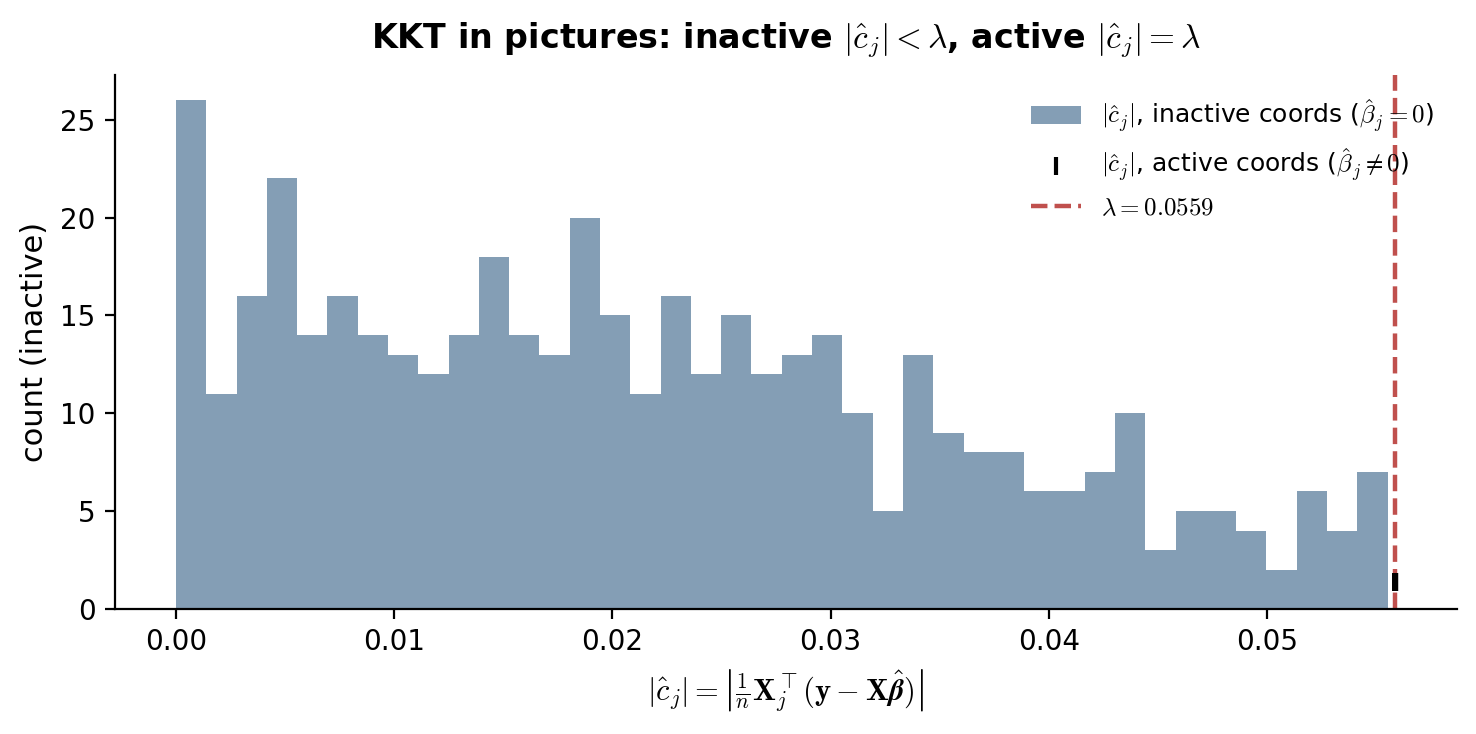
We verify the KKT conditions numerically on the §1 lasso fit at $\lambda_{\text{CV}}$: residual correlations at active coordinates equal $\pm \lambda$ to within $10^{-3}$; residual correlations at inactive coordinates are strictly bounded by $\lambda$, with the bulk well inside the dead zone.

§3. Solving the lasso

The lasso has no closed-form solution for general $\mathbf{X}$, so we need iterative algorithms. This section develops the four solvers that matter in practice, in increasing order of sophistication: the soft-thresholding closed form for orthogonal designs (§3.1, the only case that admits a closed form, but conceptually load-bearing because every general-purpose solver reduces to it inside the inner loop); coordinate descent (§3.2, the glmnet workhorse, fastest in practice for moderate-sized problems and the default in scikit-learn); ISTA, the proximal-gradient method (§3.3, simple and slow, $O(1/k)$ convergence rate, the natural first step toward FISTA); and FISTA with Nesterov momentum (§3.4, the same proximal-gradient framework with a momentum trick that improves the rate to $O(1/k^2)$, with full convergence proof). §3.5 gives practical solver-choice notes.

A common thread: every solver in this section is some application of the soft-thresholding operator $S(z, \lambda) = \mathrm{sign}(z) \cdot \max(|z| - \lambda, 0)$, the proximal operator of the L1 norm. ISTA / FISTA / coordinate descent differ only in what they soft-threshold and how often. So §3.1’s three-line derivation is the algorithmic kernel of everything that follows.

§3.1 Soft-thresholding closed form for orthogonal designs

When $\mathbf{X}^\top \mathbf{X} = n \mathbf{I}$ — an orthogonal design, achievable in practice via QR decomposition of any full-rank $\mathbf{X}$ — the lasso decouples across coordinates and admits a closed-form solution.

Substitute $\mathbf{X}^\top \mathbf{X} = n \mathbf{I}$ into the lasso objective:

$$F(\boldsymbol\beta) = \frac{1}{2n} \|\mathbf{y} - \mathbf{X} \boldsymbol\beta\|_2^2 + \lambda \|\boldsymbol\beta\|_1 = \frac{1}{2n} \|\mathbf{y}\|_2^2 - \frac{1}{n} \mathbf{y}^\top \mathbf{X} \boldsymbol\beta + \frac{1}{2} \|\boldsymbol\beta\|_2^2 + \lambda \|\boldsymbol\beta\|_1.$$

Drop the constant $\frac{1}{2n} \|\mathbf{y}\|_2^2$ and let $\mathbf{z} = \mathbf{X}^\top \mathbf{y} / n$. The objective separates by coordinate:

$$F(\boldsymbol\beta) = \mathrm{const} + \sum_{j=1}^p \left[ \frac{1}{2} (\beta_j - z_j)^2 + \lambda |\beta_j| \right] - \frac{1}{2} \|\mathbf{z}\|_2^2.$$

So the lasso reduces to $p$ independent univariate problems: minimize $\frac{1}{2}(\beta - z)^2 + \lambda |\beta|$ over $\beta \in \mathbb{R}$, one for each coordinate.

The geometric content: for each coordinate, if the (rescaled) least-squares estimate $z_j$ is small in magnitude — bounded by $\lambda$ — the lasso sets $\hat\beta_j$ to exactly zero. Otherwise, the lasso shrinks $z_j$ toward zero by exactly $\lambda$ in absolute value. The “dead zone” $|z_j| \le \lambda$ is the source of sparsity; the constant shrinkage $|\hat\beta_j| = |z_j| - \lambda$ outside the dead zone is what biases active coefficients toward zero (the bias problem the debiased lasso fixes in §10).

For non-orthogonal designs (the generic case), no closed form exists. But $S(z, \lambda)$ remains the algorithmic atom: it’s the proximal operator of the L1 norm,

$$\mathrm{prox}_{\eta \lambda \|\cdot\|_1}(\mathbf{z}) = \arg\min_{\boldsymbol\beta} \left\{ \frac{1}{2 \eta} \|\boldsymbol\beta - \mathbf{z}\|_2^2 + \lambda \|\boldsymbol\beta\|_1 \right\} = S(\mathbf{z}, \eta \lambda),$$

applied componentwise. Coordinate descent (§3.2) and proximal gradient methods (§§3.3–3.4) repeatedly apply $S(\cdot, \cdot)$ inside their iterations.

§3.2 Coordinate descent

Coordinate descent solves the lasso by cycling through coordinates and minimizing the objective over one coordinate at a time, keeping the others fixed. Each subproblem is univariate and admits a closed form via soft-thresholding.

Derivation. Fix all coordinates except $\beta_j$. The lasso objective restricted to $\beta_j$ is

$$F_j(\beta_j) = \frac{1}{2n} \|\mathbf{r}_{-j} - \mathbf{X}_j \beta_j\|_2^2 + \lambda |\beta_j| + (\text{terms not depending on } \beta_j),$$

where $\mathbf{r}_{-j} = \mathbf{y} - \sum_{k \neq j} \mathbf{X}_k \beta_k$ is the partial residual with the $j$-th feature’s contribution removed. Expand the squared loss:

$$F_j(\beta_j) = \frac{c_j}{2} \beta_j^2 - z_j \beta_j + \lambda |\beta_j| + \mathrm{const}, \quad c_j := \|\mathbf{X}_j\|_2^2 / n, \quad z_j := \mathbf{X}_j^\top \mathbf{r}_{-j} / n.$$

This is $\frac{c_j}{2}(\beta_j - z_j / c_j)^2 + \lambda |\beta_j| + \mathrm{const}'$ — the same univariate problem from §3.1 up to a rescaling. The KKT condition gives

$$\hat\beta_j^{\text{new}} = \frac{S(z_j, \lambda)}{c_j} = \frac{1}{c_j} \cdot \mathrm{sign}(z_j) \cdot \max(|z_j| - \lambda, 0).$$

Coordinate descent algorithm.

1. Initialize $\boldsymbol\beta = \mathbf{0}$, $\mathbf{r} = \mathbf{y}$.
2. For each $j = 1, 2, \dots, p$ (cyclically):
   • Form the partial residual: $\tilde{\mathbf{r}} = \mathbf{r} + \mathbf{X}_j \beta_j$.
   • Compute $z_j = \mathbf{X}_j^\top \tilde{\mathbf{r}} / n$ and $c_j = \|\mathbf{X}_j\|_2^2 / n$.
   • Update $\beta_j^{\text{new}} = S(z_j, \lambda) / c_j$.
   • Update the residual: $\mathbf{r} \leftarrow \mathbf{r} - \mathbf{X}_j (\beta_j^{\text{new}} - \beta_j)$, then $\beta_j \leftarrow \beta_j^{\text{new}}$.
3. Repeat step 2 until $\|\boldsymbol\beta^{\text{old}} - \boldsymbol\beta^{\text{new}}\|$ falls below tolerance.

Why the residual update. Storing $\mathbf{r}$ and updating it incrementally avoids re-computing $\mathbf{X} \boldsymbol\beta$ from scratch at each coordinate update. Each update costs $O(n)$ instead of $O(np)$, so a full cycle costs $O(np)$ — the same as one ISTA / FISTA iteration.

Convergence. The lasso objective is the sum of a smooth strictly-convex (in $\mathbf{X} \boldsymbol\beta$) quadratic and a separable convex term $\lambda \sum_j |\beta_j|$. Tseng (2001) showed that block coordinate descent converges to a global minimum for any objective of this form (smooth + separable convex), with no rate guarantee in general but linear convergence under additional assumptions. In practice on lasso problems with continuous designs, coordinate descent is one of the fastest methods — Friedman, Hastie & Tibshirani (2010) report 10–100× speedups over LARS and proximal-gradient methods at typical $(n, p)$ scales. The glmnet package and scikit-learn’s Lasso both use it as the default.

Warm starts along a $\lambda$ path. Practical solvers compute the lasso path $\hat{\boldsymbol\beta}(\lambda)$ for a decreasing grid of $\lambda$ values, using the previous solution as a warm start at the next $\lambda$. The path is piecewise linear in $\lambda$ (Efron-Hastie-Johnstone-Tibshirani 2004), so a small step in $\lambda$ requires few coordinate-descent passes to converge — typically 5–20.

§3.3 ISTA: the proximal gradient method

Coordinate descent works for the lasso because the L1 penalty is separable. For more general non-smooth penalties (group lasso, fused lasso, nuclear norm), we need a different framework. Proximal gradient methods generalize gradient descent to objectives of the form $F(\boldsymbol\beta) = f(\boldsymbol\beta) + g(\boldsymbol\beta)$, where $f$ is smooth and $g$ is non-smooth but admits a tractable proximal operator. For the lasso, $f(\boldsymbol\beta) = (1/2n) \|\mathbf{y} - \mathbf{X} \boldsymbol\beta\|_2^2$ and $g(\boldsymbol\beta) = \lambda \|\boldsymbol\beta\|_1$, with $\mathrm{prox}_{\eta g}(\mathbf{z}) = S(\mathbf{z}, \eta \lambda)$.

The iterative soft-thresholding algorithm (ISTA) is the proximal-gradient iteration:

$$\boldsymbol\beta^{k+1} = \mathrm{prox}_{\eta g}(\boldsymbol\beta^k - \eta \nabla f(\boldsymbol\beta^k)) = S\!\left( \boldsymbol\beta^k - \frac{\eta}{n} \mathbf{X}^\top (\mathbf{X} \boldsymbol\beta^k - \mathbf{y}), \; \eta \lambda \right),$$

with a step size $\eta = 1/L$ where $L = \|\mathbf{X}\|_2^2 / n$ is the Lipschitz constant of $\nabla f$ (largest eigenvalue of $\mathbf{X}^\top \mathbf{X} / n$). Each iteration costs one matrix-vector multiply $\mathbf{X} \boldsymbol\beta^k$ and one $\mathbf{X}^\top \mathbf{r}$ — the same $O(np)$ as a coordinate-descent cycle.

The $O(1/k)$ rate is “sublinear” — to halve the suboptimality $F(\boldsymbol\beta^k) - F^*$ requires doubling $k$. ISTA is simple and stable but slow.

§3.4 FISTA: Nesterov momentum and the $O(1/k^2)$ rate

Beck-Teboulle (2009) showed that adding Nesterov momentum to ISTA accelerates the convergence rate from $O(1/k)$ to $O(1/k^2)$ — a quadratic improvement in iteration count for the same accuracy. The algorithm:

FISTA. Set $\boldsymbol\beta^0 = \boldsymbol\beta^{-1} = \mathbf{0}$, $t_1 = 1$. For $k = 1, 2, \dots$:

1. $\mathbf{z}^k = \boldsymbol\beta^k + \frac{t_k - 1}{t_{k+1}} (\boldsymbol\beta^k - \boldsymbol\beta^{k-1})$ — momentum extrapolation.
2. $\boldsymbol\beta^{k+1} = S\!\left( \mathbf{z}^k - \frac{1}{nL} \mathbf{X}^\top (\mathbf{X} \mathbf{z}^k - \mathbf{y}), \; \lambda / L \right)$ — proximal gradient step from $\mathbf{z}^k$, not $\boldsymbol\beta^k$.
3. $t_{k+1} = (1 + \sqrt{1 + 4 t_k^2}) / 2$.

The momentum coefficient $(t_k - 1)/t_{k+1}$ approaches $1$ as $k$ grows, giving the iteration a “running start” along the previous direction of motion.

A factor-of-$k$ improvement over ISTA: to reduce $F(\boldsymbol\beta^k) - F^*$ by a factor of 100, ISTA needs 100× more iterations while FISTA needs only 10×. The constant $2L \|\boldsymbol\beta^0 - \boldsymbol\beta^*\|^2$ is the same as the ISTA bound (modulo the factor of 4), so the asymptotic rate is the only source of difference — but it’s a substantial one.

FISTA is not a descent method. Unlike ISTA, $F(\boldsymbol\beta^k)$ is not monotonic along FISTA iterations — small “ripples” in $F(\boldsymbol\beta^k)$ are normal. A monotone variant (M-FISTA, Beck-Teboulle 2009 §5) accepts $\boldsymbol\beta^{k+1}$ only if $F(\boldsymbol\beta^{k+1}) \le F(\boldsymbol\beta^k)$, otherwise reuses $\boldsymbol\beta^k$. This trade-off — slightly worse worst-case constant for monotonicity — is rarely worth it in practice.

Log-log convergence trace on a smaller-scale DGP-1 (n = 150, p = 200, s = 10, σ = 0.5, AR(1) ρ = 0.5) at λ = 0.05. F* is computed by a 5,000-iteration FISTA reference. Reading off the slopes: ISTA tracks k⁻¹ (Theorem 3.2), FISTA tracks k⁻² (Theorem 3.3), and coordinate descent matches FISTA early then asymptotically beats both once the active set stabilizes — the lasso restricted to a fixed active set is a strictly-convex quadratic, where CD converges linearly. Iterations to reach F − F* < 10⁻³: ISTA = 63, FISTA = 22, CD = 6.

§3.5 Practical solver-choice notes

When does each solver win? A field guide.

Coordinate descent (sklearn.linear_model.Lasso, glmnet). Default for everything in the lasso family (lasso, elastic net, group lasso). Fastest in practice for $n, p \le 10^5$ at moderate sparsity. Warm starts along a $\lambda$ path are nearly free, which is why LassoCV is fast even with 100-fold path × 10-fold CV.

FISTA. The right default for lasso variants where the L1 prox is easy but coordinate-by-coordinate updates are not — group lasso with overlapping groups, fused lasso, generalized-lasso-with-non-axis-aligned penalty, total-variation penalties. Also the right default when the design matrix is structured (e.g., a fast Fourier or wavelet transform) and matrix-vector products $\mathbf{X} \mathbf{v}$ can be computed in $O(n \log n)$ rather than $O(np)$ — coordinate descent breaks the structured-multiplication advantage by accessing one column at a time.

ISTA. Pedagogically valuable, rarely the right algorithmic choice — FISTA dominates it at no extra implementation cost. Use ISTA only when the proof of correctness or the descent property is needed (some monotonicity-sensitive applications, e.g., in statistical guarantees that rely on objective decrease).

Specialized solvers we don’t cover. ADMM (Boyd et al. 2011) is the right tool for lasso variants with linear-equality-coupled penalties (e.g., the Dantzig selector). LARS (Efron-Hastie-Johnstone-Tibshirani 2004) computes the entire lasso path exactly in $O(np \min(n, p))$, which can beat coordinate descent at very small $p$ but loses badly at the high-dimensional scales we care about. Interior-point methods (CVXPY, cvxopt) work but are typically 100×+ slower than coordinate descent on lasso problems of any meaningful size.

For everything in the rest of this topic — the §1 lasso fits, the LassoCV in §7, the elastic-net comparison in §8, the debiased-lasso pipeline in §10 — we use scikit-learn’s coordinate descent. We hand-rolled FISTA above to demonstrate the $O(1/k^2)$ rate and to keep the algorithmic content visible.

§4. Bias-variance for the lasso

The lasso’s central trade-off is between bias (from L1 shrinkage of active coefficients) and variance (controlled by the size of the data-adapted active set). As $\lambda$ ranges from $0$ to $\lambda_{\max}$ — the smallest penalty at which the solution is identically zero — the prediction risk traces the canonical U-curve familiar from any bias-variance analysis. This section formalizes both halves of the trade-off, computes $\lambda_{\max}$ in closed form from the KKT conditions, and develops the lasso solution path $\hat{\boldsymbol\beta}(\lambda)$ as a piecewise-linear function of $\lambda$.

The U-curve is the practical bridge between §3 (we can compute the lasso) and §5 (the oracle inequality bounds the bottom of the U). The solution path is what LassoCV (§7) and LassoLarsIC (§7) operate on when they pick a $\lambda$.

§4.1 The bias contribution from L1 shrinkage

The lasso’s shrinkage isn’t soft and asymptotically vanishing the way a Bayesian Gaussian-prior posterior is — it’s a constant absolute shrinkage that biases every active coefficient toward zero by approximately $\lambda$.

The orthogonal case makes this explicit. From §3.1, with $\mathbf{X}^\top \mathbf{X} = n \mathbf{I}$ and $z_j = (\mathbf{X}^\top \mathbf{y} / n)_j$, the lasso solution is $\hat\beta_j = S(z_j, \lambda)$. Under the model $z_j \sim \mathcal{N}(\beta^*_j, \sigma^2 / n)$:

• For “large signal” coordinates with $|\beta^*_j| \gg \lambda + \sigma/\sqrt{n}$: with high probability $|z_j| > \lambda$ and $\mathrm{sign}(z_j) = \mathrm{sign}(\beta^*_j)$, so $\hat\beta_j \approx z_j - \lambda \, \mathrm{sign}(\beta^*_j)$ and $\mathbb{E}[\hat\beta_j] \approx \beta^*_j - \lambda \, \mathrm{sign}(\beta^*_j)$. The bias is $-\lambda \, \mathrm{sign}(\beta^*_j)$ — constant magnitude, opposite sign to the true value, independent of how large $\beta^*_j$ is.
• For “noise” coordinates with $\beta^*_j = 0$: by the symmetry $z_j \sim \mathcal{N}(0, \sigma^2/n)$, $\mathbb{E}[S(z_j, \lambda)] = 0$. No bias, but a small variance contribution from the false positives where $|z_j| > \lambda$ by chance.

For general (non-orthogonal) designs, the calculation is more involved but the qualitative picture survives. Conditioning on the lasso correctly identifying the active set $S$, the active coefficients satisfy

$$\hat{\boldsymbol\beta}_S = \hat{\boldsymbol\beta}_S^{\text{OLS-on-}S} - \lambda \big(\mathbf{X}_S^\top \mathbf{X}_S / n\big)^{-1} \mathrm{sign}(\hat{\boldsymbol\beta}_S),$$

where $\hat{\boldsymbol\beta}_S^{\text{OLS-on-}S} = (\mathbf{X}_S^\top \mathbf{X}_S)^{-1} \mathbf{X}_S^\top \mathbf{y}$ is the OLS estimator restricted to $S$. The shrinkage correction $-\lambda (\mathbf{X}_S^\top \mathbf{X}_S / n)^{-1} \mathrm{sign}(\cdot)$ scales linearly in $\lambda$; its magnitude depends on the conditioning of $\mathbf{X}_S^\top \mathbf{X}_S / n$ but is generally of order $\lambda$.

This bias is the price of sparsity. Two later sections fix it for different reasons:

• The adaptive lasso (Zou 2006, §8.3) replaces the constant shrinkage $\lambda$ with feature-specific weights $\lambda \cdot w_j$ where $w_j = 1 / |\hat\beta_j^{\text{init}}|$ for some initial estimator. Coordinates with large $|\hat\beta_j^{\text{init}}|$ get small $w_j$ and small shrinkage, so the active-coefficient bias decays to zero asymptotically.
• The debiased lasso (§10.2) explicitly subtracts off the shrinkage bias via a one-step Newton correction $\hat{\boldsymbol\beta}^{\text{db}} = \hat{\boldsymbol\beta} + (1/n) \hat{\mathbf{M}} \mathbf{X}^\top (\mathbf{y} - \mathbf{X} \hat{\boldsymbol\beta})$, producing $\sqrt{n}$-consistent normal estimates of individual coefficients suitable for hypothesis testing and confidence intervals.

For prediction the bias isn’t catastrophic — the U-curve in §4.3 shows that the bias-variance trade-off is favorable at well-chosen $\lambda$. For inference it’s the central problem of the topic, and §10 is where it gets resolved.

§4.2 Variance from sparsity adaptation

In contrast to the bias, the lasso’s variance is small — much smaller than the variance of OLS would be at the same $p$, when OLS is even defined.

The cleanest way to see this: OLS variance scales with the number of features, $\mathbb{V}\mathrm{ar}(\hat{\boldsymbol\beta}^{\text{OLS}}) = \sigma^2 (\mathbf{X}^\top \mathbf{X})^{-1}$ has trace $\sigma^2 \, \mathrm{tr}((\mathbf{X}^\top \mathbf{X})^{-1})$, which scales as $\sigma^2 p / n$ for a well-conditioned design. As $p \to n$ from below, the variance blows up; at $p > n$, OLS is undefined and the min-norm interpolant has its own pathologies.

The lasso, by zeroing out coordinates with small $|z_j|$, effectively reduces the model dimension from $p$ to the active-set size $|\hat A_\lambda|$. Heuristically — and this is made precise by the degrees of freedom of the lasso result (Zou-Hastie-Tibshirani 2007): $\mathrm{df}(\hat{\boldsymbol\beta}^{\text{lasso}}(\lambda)) = \mathbb{E}[|\hat A_\lambda|]$, the expected size of the active set. So the lasso’s prediction variance scales as $\sigma^2 \, \mathbb{E}[|\hat A_\lambda|] / n$, which for a well-chosen $\lambda$ is on the order of $\sigma^2 s / n$ — proportional to the true sparsity, not to $p$.

This is the sparsity-adaptation property: the lasso pays a variance cost proportional to the model size it actually uses, regardless of how many candidate features were available to start with. It’s the central reason the lasso works in the $p \gg n$ regime where OLS doesn’t.

For DGP-1 with $s = 10$, $\sigma = 0.5$, $n = 200$: the lasso variance is roughly $\sigma^2 s / n = 0.0125$, while OLS at $p = 199$ has variance roughly $\sigma^2 \cdot 199 / 200 \approx 0.249$ — a 20× advantage, before counting the bias.

§4.3 The U-curve as $\lambda$ varies

The bias-variance pieces combine into the canonical U-shaped prediction-risk curve as a function of $\lambda$. Define the prediction risk at test point $\mathbf{x}^*$:

$$R(\lambda; \mathbf{x}^*) := \mathbb{E}\big[ (\mathbf{x}^{*\top} \hat{\boldsymbol\beta}(\lambda) - \mathbf{x}^{*\top} \boldsymbol\beta^*)^2 \big] = \underbrace{\big(\mathbb{E}[\mathbf{x}^{*\top} \hat{\boldsymbol\beta}(\lambda)] - \mathbf{x}^{*\top} \boldsymbol\beta^*\big)^2}_{\text{bias}^2(\mathbf{x}^*; \lambda)} + \underbrace{\mathbb{V}\mathrm{ar}(\mathbf{x}^{*\top} \hat{\boldsymbol\beta}(\lambda))}_{\text{variance}(\mathbf{x}^*; \lambda)},$$

with the expectation over training-set draws (test point $\mathbf{x}^*$ fixed). Average over $\mathbf{x}^*$ in a test set to get the integrated prediction risk $\mathrm{IPE}(\lambda) = \mathbb{E}_{\mathbf{x}^*}[R(\lambda; \mathbf{x}^*)]$.

The U-curve has two boundaries:

• At $\lambda = 0$ (OLS / min-norm OLS at $p > n$): bias is zero (or near-zero for min-norm) but variance dominates and is large or undefined.
• At $\lambda = \lambda_{\max}$ (defined below): variance is zero — $\hat{\boldsymbol\beta}(\lambda) = \mathbf{0}$ deterministically — but bias equals the full prediction signal $\mathbf{x}^{*\top} \boldsymbol\beta^*$, so bias² is large.

Between these endpoints the curve is U-shaped, with an optimal $\lambda^*$ that minimizes IPE. The §5 oracle inequality bounds the value of IPE at this optimum from above by $C \sigma^2 s \log(p) / n$.

$\lambda_{\max}$ in closed form. From the KKT conditions of §2.4: $\hat{\boldsymbol\beta} = \mathbf{0}$ is a lasso solution if and only if $|(\mathbf{X}^\top \mathbf{y} / n)_j| \le \lambda$ for all $j$ — i.e., the inactive condition holds at every coordinate. So

$$\lambda_{\max} = \left\| \frac{\mathbf{X}^\top \mathbf{y}}{n} \right\|_\infty = \max_j \left| \frac{\mathbf{X}_j^\top \mathbf{y}}{n} \right|.$$

For $\lambda \ge \lambda_{\max}$, the lasso solution is identically zero. For $\lambda$ just below $\lambda_{\max}$, exactly one coordinate becomes active (the one achieving the maximum) — this is the start of the lasso path described next. On DGP-1 with seed 42, $\lambda_{\max} \approx 1.04$, and $\lambda_{\text{CV}} \approx 0.06$ sits two orders of magnitude smaller — well into the path’s interesting region.

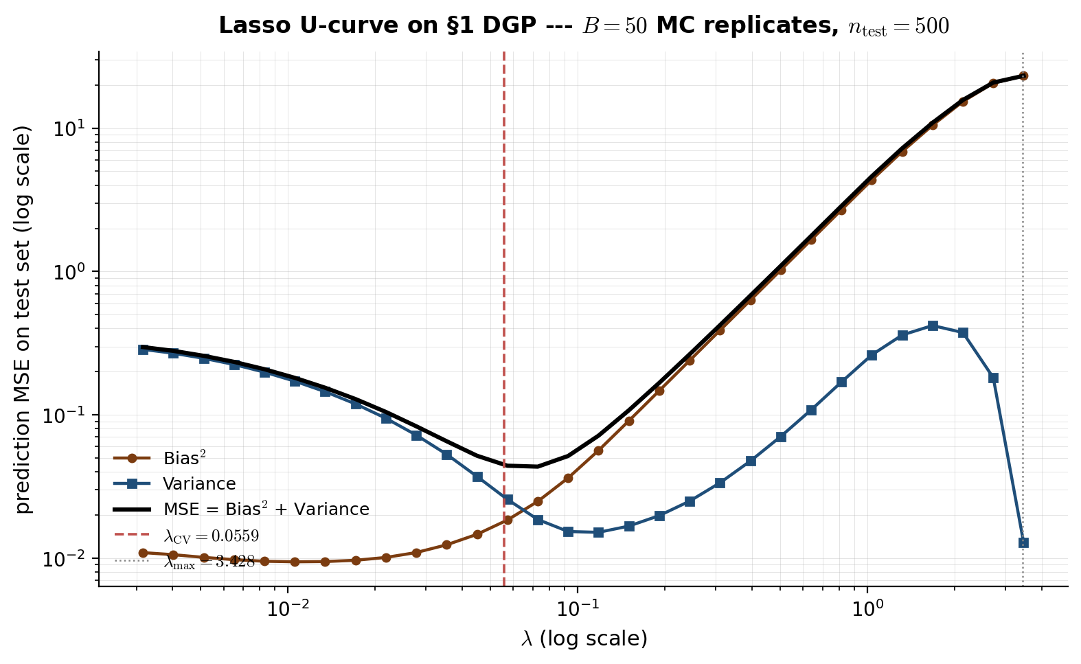
The interactive viz below shows empirical bias², variance, and total MSE on a held-out test set as a function of $\lambda$, computed by Monte Carlo over $B$ replicate draws of DGP-1. Bias² grows monotonically with $\lambda$ (constant shrinkage hurts more when applied harder); variance decays monotonically with $\lambda$ (heavier penalization shrinks the active set); their sum traces a U-curve with minimum near $\lambda_{\text{CV}}$. The minimum of the empirical U-curve coincides — within MC noise — with the value of $\lambda$ that LassoCV selects automatically (§7).

Empirical bias-variance decomposition on a smaller-scale DGP-1 (n = 200, p = 200, s = 10, σ = 0.5, AR(1) ρ = 0.5, B = 20 replicates). MSE = bias² + variance is the canonical U; bias² (teal, dashed) grows with λ as constant shrinkage hits active coords harder; variance (purple, dotted) decays with λ as the active-set size shrinks. The red marker sits at the empirical λ minimizer of MSE — close to the LassoCV-selected operating point covered in §7. Computed live in-browser via warm-started ISTA across the 25-point log-spaced λ-grid (~3-5 s precompute).

§4.4 The lasso solution path is piecewise linear

Define the lasso solution path as the function $\lambda \mapsto \hat{\boldsymbol\beta}(\lambda)$ for $\lambda \in [0, \lambda_{\max}]$. The path has two structural properties that make it both computationally tractable and visually informative.

The proof is a direct calculation from the KKT conditions: between knots, the active set is fixed, the active KKT condition $\frac{1}{n} \mathbf{X}_j^\top (\mathbf{y} - \mathbf{X} \hat{\boldsymbol\beta}) = \lambda \, \mathrm{sign}(\hat\beta_j)$ for $j \in \hat A$ is a linear system in $\hat{\boldsymbol\beta}_{\hat A}$ with $\lambda$ on the right-hand side, so the solution is linear in $\lambda$. The LARS algorithm (Efron et al. 2004) traces this piecewise-linear path knot-by-knot in $O(np \min(n, p))$ total time — though for moderate-to-large $p$, coordinate descent on a $\lambda$-grid (§3.2) is faster in practice.

Reading the path. Plotting $\hat\beta_j(\lambda)$ vs $\log \lambda$ for all $j$ shows which features the lasso selects in what order and at what penalty level. As $\lambda$ decreases from $\lambda_{\max}$:

• The first coordinate to enter is $\arg\max_j |(\mathbf{X}^\top \mathbf{y} / n)_j|$ — the feature most correlated with the response.
• Subsequent coordinates enter at successively smaller $\lambda$ values, in roughly the order of their importance.
• At $\lambda = 0$ the path reaches OLS (in the $p \le n$ case) or the min-norm OLS interpolant (in $p > n$).
• A coordinate can also leave the active set as $\lambda$ decreases (coefficient passes through zero) — uncommon in continuous designs but possible.

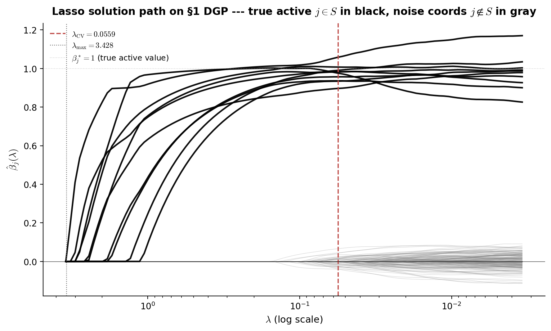
The viz below shows the lasso solution path on DGP-1: $\hat\beta_j(\lambda)$ vs $\log \lambda$ for all 500 coordinates, with the 10 true active coordinates plotted in black and the 490 inactive coordinates in light gray. The vertical line at $\lambda_{\text{CV}}$ marks the cross-validation-selected operating point. The reader sees that the true active features are consistently the first to enter the path as $\lambda$ decreases, and that at $\lambda_{\text{CV}}$ the active set is a tight superset of the true $S$ — most of the gray noise coefficients are still at zero.

Lasso solution path on a smaller-scale DGP-1 (n = 200, p = 200, s = 10, σ = 0.5, AR(1) ρ = 0.5). The 10 true active coordinates (j < 10) plot in black; the 190 inactive coordinates in gray (only those with |β̂_j| > 0.005 anywhere on the path are drawn — most stay flat-zero and are omitted to keep the SVG light). Vertical marker at λ_CV ≈ 0.056 (the LassoUCurve minimizer above). The active features enter the path first as λ decreases from λ_max ≈ 1; at λ_CV the active set is a tight superset of the true S. Computed live via warm-started ISTA across 30 log-spaced λ values (~200 ms precompute).

§5. The lasso oracle inequality

This is the topic’s headline theoretical result: under a restricted-eigenvalue condition on the design and a deviation bound on the noise, the lasso achieves prediction risk of order $\sigma^2 s \log(p) / n$ — comparable to what an oracle that knew the true active set $S$ in advance could achieve, up to a logarithmic factor in $p$. The bound is non-asymptotic (holds with high probability for any finite $n$, $p$), dimension-free (the dependence on $p$ is only logarithmic), and rate-optimal for the sparse high-dimensional regression problem.

The proof has four steps and follows Bickel-Ritov-Tsybakov (2009) closely. Step 1 (the basic inequality) uses the lasso’s defining optimality to bound the prediction error in terms of the L1 estimation error and a noise term. Step 2 (the cone condition) shows that the error vector $\hat{\boldsymbol\beta} - \boldsymbol\beta^*$ has most of its L1 mass concentrated on the true support $S$. Step 3 (the restricted-eigenvalue condition) lets us convert L1 estimation error on $S$ into a lower bound on the prediction error. Step 4 (the deviation step) controls the noise term using a maximal sub-Gaussian inequality. Combining gives the rate.

The proof’s main work is in steps 1 and 2 — the basic inequality and the cone condition derive directly from the KKT conditions of §2.4 with no further ingredients. Step 3 is the geometric assumption on the design that we’re imposing; step 4 is the standard probabilistic deviation inequality. The whole argument is technical but elementary — no measure theory beyond the sub-Gaussian moment bound.

§5.1 Setup: prediction risk in the high-dim regime

We work in the standard high-dimensional linear regression model:

$$\mathbf{y} = \mathbf{X} \boldsymbol\beta^* + \boldsymbol\varepsilon, \quad \mathbf{X} \in \mathbb{R}^{n \times p}, \quad \boldsymbol\beta^* \in \mathbb{R}^p, \quad \boldsymbol\varepsilon \in \mathbb{R}^n.$$

We assume:

• Sparsity. $\boldsymbol\beta^*$ has support $S = \{j : \beta^*_j \neq 0\}$ with $|S| = s$, $s \ll p$.
• Sub-Gaussian noise. $\boldsymbol\varepsilon = (\varepsilon_1, \dots, \varepsilon_n)$ has independent entries with $\mathbb{E}[\varepsilon_i] = 0$ and sub-Gaussian parameter $\sigma$: $\mathbb{E}[\exp(t \varepsilon_i)] \le \exp(t^2 \sigma^2 / 2)$ for all $t \in \mathbb{R}$. Gaussian noise with variance $\sigma^2$ is the canonical case; bounded $\boldsymbol\varepsilon \in [-\sigma, \sigma]$ also qualifies.
• Column-normalized design. Each column $\mathbf{X}_j$ satisfies $\|\mathbf{X}_j\|_2^2 \le n$ — a normalization convention that makes the bound clean. Equivalently, the empirical second moment $(1/n) \|\mathbf{X}_j\|_2^2 \le 1$. For DGP-1 the columns satisfy this in expectation; in practice rescaling the columns to exactly $\|\mathbf{X}_j\|_2^2 = n$ is standard before fitting.

The prediction risk at the lasso estimator is

$$\mathrm{PE}(\hat{\boldsymbol\beta}^{\text{lasso}}) := \frac{1}{n} \|\mathbf{X} (\hat{\boldsymbol\beta}^{\text{lasso}} - \boldsymbol\beta^*)\|_2^2 = \frac{1}{n} \sum_{i=1}^n (\mathbf{x}_i^\top \hat{\boldsymbol\beta}^{\text{lasso}} - \mathbf{x}_i^\top \boldsymbol\beta^*)^2,$$

the average squared in-sample prediction error against the true regression function. (This is the “fixed-design prediction error.” It differs from the integrated $\mathbb{E}_{\mathbf{x}^*}[\cdot]$ test-set error of §4.3 — they coincide when the test design has the same row distribution as the training design and $n$ is large.)

The benchmark is the oracle estimator that knew $S$ in advance:

$$\hat{\boldsymbol\beta}^{\text{oracle}}_S = (\mathbf{X}_S^\top \mathbf{X}_S)^{-1} \mathbf{X}_S^\top \mathbf{y}, \qquad \hat{\boldsymbol\beta}^{\text{oracle}}_{S^c} = \mathbf{0}.$$

The oracle is OLS restricted to $S$. Its prediction risk is $\mathrm{PE}(\hat{\boldsymbol\beta}^{\text{oracle}}) = \sigma^2 s / n$ in expectation (standard OLS variance with $s$ degrees of freedom). The oracle inequality says the lasso achieves the same rate up to a $\log(p)$ factor, without knowing $S$.

§5.2 The basic inequality

The starting point is the lasso’s defining optimality: $\hat{\boldsymbol\beta}^{\text{lasso}}$ achieves the minimum of the lasso objective, so in particular it does no worse than $\boldsymbol\beta^*$:

$$\frac{1}{2n} \|\mathbf{y} - \mathbf{X} \hat{\boldsymbol\beta}\|_2^2 + \lambda \|\hat{\boldsymbol\beta}\|_1 \le \frac{1}{2n} \|\mathbf{y} - \mathbf{X} \boldsymbol\beta^*\|_2^2 + \lambda \|\boldsymbol\beta^*\|_1.$$

(We drop the “lasso” superscript for brevity; $\hat{\boldsymbol\beta}$ is always the lasso solution in this section.)

Substitute $\mathbf{y} = \mathbf{X} \boldsymbol\beta^* + \boldsymbol\varepsilon$ and let $\boldsymbol\delta = \hat{\boldsymbol\beta} - \boldsymbol\beta^*$:

$$\frac{1}{2n} \|\mathbf{X} \boldsymbol\beta^* + \boldsymbol\varepsilon - \mathbf{X} \hat{\boldsymbol\beta}\|_2^2 = \frac{1}{2n} \|\boldsymbol\varepsilon - \mathbf{X} \boldsymbol\delta\|_2^2 = \frac{1}{2n} \|\boldsymbol\varepsilon\|_2^2 - \frac{1}{n} \boldsymbol\varepsilon^\top \mathbf{X} \boldsymbol\delta + \frac{1}{2n} \|\mathbf{X} \boldsymbol\delta\|_2^2,$$

and $\frac{1}{2n} \|\mathbf{y} - \mathbf{X} \boldsymbol\beta^*\|_2^2 = \frac{1}{2n} \|\boldsymbol\varepsilon\|_2^2$. The $\frac{1}{2n}\|\boldsymbol\varepsilon\|_2^2$ terms cancel, giving

$$\frac{1}{2n} \|\mathbf{X} \boldsymbol\delta\|_2^2 - \frac{1}{n} \boldsymbol\varepsilon^\top \mathbf{X} \boldsymbol\delta + \lambda \|\hat{\boldsymbol\beta}\|_1 \le \lambda \|\boldsymbol\beta^*\|_1.$$

Rearrange and double both sides:

$$\frac{1}{n} \|\mathbf{X} \boldsymbol\delta\|_2^2 \le \frac{2}{n} \boldsymbol\varepsilon^\top \mathbf{X} \boldsymbol\delta + 2\lambda \big( \|\boldsymbol\beta^*\|_1 - \|\hat{\boldsymbol\beta}\|_1 \big). \quad\quad (\star)$$

This is the basic inequality. Two things to control: the noise inner product $\boldsymbol\varepsilon^\top \mathbf{X} \boldsymbol\delta / n$, and the L1-norm difference $\|\boldsymbol\beta^*\|_1 - \|\hat{\boldsymbol\beta}\|_1$.

The noise term, via Hölder’s inequality.

$$\frac{2}{n} |\boldsymbol\varepsilon^\top \mathbf{X} \boldsymbol\delta| = 2 \left| \frac{\boldsymbol\varepsilon^\top \mathbf{X}}{n} \boldsymbol\delta \right| \le 2 \left\| \frac{\mathbf{X}^\top \boldsymbol\varepsilon}{n} \right\|_\infty \cdot \|\boldsymbol\delta\|_1.$$

Define the noise event

$$\mathcal{E} := \left\{ \left\| \frac{\mathbf{X}^\top \boldsymbol\varepsilon}{n} \right\|_\infty \le \frac{\lambda}{2} \right\}.$$

On $\mathcal{E}$, $(2/n) \boldsymbol\varepsilon^\top \mathbf{X} \boldsymbol\delta \le \lambda \|\boldsymbol\delta\|_1$. Step 4 below shows that with $\lambda$ chosen as $\lambda = 2\sigma \sqrt{2 \log(2p/\delta) / n}$, the event $\mathcal{E}$ holds with probability at least $1 - \delta$. For now assume we’re on $\mathcal{E}$.

The L1-norm difference, via the support split. Decompose $\hat{\boldsymbol\beta} = \hat{\boldsymbol\beta}_S + \hat{\boldsymbol\beta}_{S^c}$ where the subscripts indicate the indices restricted to $S$ and $S^c$ respectively. Since $\boldsymbol\beta^*_{S^c} = \mathbf{0}$:

$$\|\boldsymbol\beta^*\|_1 = \|\boldsymbol\beta^*_S\|_1, \qquad \|\hat{\boldsymbol\beta}\|_1 = \|\hat{\boldsymbol\beta}_S\|_1 + \|\hat{\boldsymbol\beta}_{S^c}\|_1, \qquad \|\boldsymbol\delta\|_1 = \|\hat{\boldsymbol\beta}_S - \boldsymbol\beta^*_S\|_1 + \|\hat{\boldsymbol\beta}_{S^c}\|_1.$$

Apply the reverse triangle inequality $\|\hat{\boldsymbol\beta}_S\|_1 \ge \|\boldsymbol\beta^*_S\|_1 - \|\hat{\boldsymbol\beta}_S - \boldsymbol\beta^*_S\|_1$:

$$\|\boldsymbol\beta^*\|_1 - \|\hat{\boldsymbol\beta}\|_1 = \|\boldsymbol\beta^*_S\|_1 - \|\hat{\boldsymbol\beta}_S\|_1 - \|\hat{\boldsymbol\beta}_{S^c}\|_1 \le \|\hat{\boldsymbol\beta}_S - \boldsymbol\beta^*_S\|_1 - \|\hat{\boldsymbol\beta}_{S^c}\|_1 = \|\boldsymbol\delta_S\|_1 - \|\boldsymbol\delta_{S^c}\|_1.$$

Substitute into $(\star)$ on the event $\mathcal{E}$:

$$\frac{1}{n} \|\mathbf{X} \boldsymbol\delta\|_2^2 \le \lambda \|\boldsymbol\delta\|_1 + 2\lambda (\|\boldsymbol\delta_S\|_1 - \|\boldsymbol\delta_{S^c}\|_1) = 3\lambda \|\boldsymbol\delta_S\|_1 - \lambda \|\boldsymbol\delta_{S^c}\|_1.$$

Combining the $\boldsymbol\delta_S$ and $\boldsymbol\delta_{S^c}$ terms:

$$\boxed{\; \frac{1}{n} \|\mathbf{X} \boldsymbol\delta\|_2^2 + \lambda \|\boldsymbol\delta_{S^c}\|_1 \le 3\lambda \|\boldsymbol\delta_S\|_1 \;} \quad \text{on } \mathcal{E}. \quad\quad (\star\star)$$

This is the basic inequality in its useful form. The L1 mass of $\boldsymbol\delta$ outside the true support, plus the prediction error, is controlled by the L1 mass on the true support.

§5.3 The cone condition

The basic inequality $(\star\star)$ has an immediate geometric consequence. The prediction-error term $\frac{1}{n}\|\mathbf{X}\boldsymbol\delta\|_2^2$ on the LHS is non-negative, so we can drop it:

$$\lambda \|\boldsymbol\delta_{S^c}\|_1 \le 3\lambda \|\boldsymbol\delta_S\|_1 \quad \Rightarrow \quad \boxed{\;\|\boldsymbol\delta_{S^c}\|_1 \le 3 \|\boldsymbol\delta_S\|_1.\;}$$

This is the cone condition. The error vector $\boldsymbol\delta = \hat{\boldsymbol\beta} - \boldsymbol\beta^*$ lies in the convex cone

$$\mathcal{C}(S, 3) := \{ \boldsymbol\delta \in \mathbb{R}^p : \|\boldsymbol\delta_{S^c}\|_1 \le 3 \|\boldsymbol\delta_S\|_1 \}.$$

Interpretation. Most of the error vector’s L1 mass is on the true support $S$. The factor of 3 is conventional; it depends on the constant 2 in the basic inequality, which in turn comes from doubling both sides of the lasso optimality. Different works in the literature use $\mathcal{C}(S, c_0)$ for various $c_0 \ge 1$; the bound just needs the cone constant to be finite.

The cone condition is the structural content of the basic inequality. Without any further assumption on $\mathbf{X}$ or $\boldsymbol\varepsilon$, we know the lasso error is concentrated on $S$ — but we don’t yet have a rate bound on the prediction error. The next step requires an additional assumption on the design.

§5.4 The restricted-eigenvalue condition

The pure basic inequality $(\star\star)$ gives $\frac{1}{n}\|\mathbf{X}\boldsymbol\delta\|_2^2 \le 3\lambda \|\boldsymbol\delta_S\|_1$. The RHS bounds the prediction error in terms of the L1 norm of the active part of $\boldsymbol\delta$, which has only $s$ entries — so by Cauchy-Schwarz, $\|\boldsymbol\delta_S\|_1 \le \sqrt{s} \|\boldsymbol\delta_S\|_2$. We get

$$\frac{1}{n} \|\mathbf{X} \boldsymbol\delta\|_2^2 \le 3\lambda \sqrt{s} \|\boldsymbol\delta_S\|_2.$$

To convert this into a rate bound, we need to bound $\|\boldsymbol\delta_S\|_2$ from above by something involving $\frac{1}{n}\|\mathbf{X}\boldsymbol\delta\|_2^2$ — i.e., a lower bound on $\frac{1}{n}\|\mathbf{X}\boldsymbol\delta\|_2^2$ in terms of $\|\boldsymbol\delta_S\|_2^2$. That’s exactly the restricted-eigenvalue condition.

In words: on the cone $\mathcal{C}(S, c_0)$, the empirical Gram matrix $\mathbf{X}^\top \mathbf{X} / n$ acts like a positive-definite matrix on the active block — its smallest “eigenvalue” restricted to $\mathcal{C}(S, c_0)$ is at least $\kappa^2$. On the full space $\mathbb{R}^p$ this would be the smallest eigenvalue of $\mathbf{X}^\top \mathbf{X}/n$, which is zero whenever $p > n$. The restriction to the cone $\mathcal{C}(S, c_0)$ is what makes the condition feasible in the high-dim regime.

When does RE hold? A few sufficient conditions:

• Random Gaussian designs. If $\mathbf{X}$ has iid $\mathcal{N}(\mathbf{0}, \boldsymbol\Sigma)$ rows with $\lambda_{\min}(\boldsymbol\Sigma) \ge \kappa_0^2 > 0$, then RE holds with high probability with $\kappa^2 \asymp \kappa_0^2$ provided $n \gtrsim s \log(p)$ (Raskutti-Wainwright-Yu 2010, Theorem 1).
• Sub-Gaussian designs. Same conclusion under sub-Gaussian rows (Rudelson-Zhou 2013).
• Restricted isometry property (RIP). RIP $\Rightarrow$ RE (Candès-Tao 2005; we cover this in §9).

The condition is essentially the weakest design assumption under which the lasso works — it’s equivalent to ”$\mathbf{X}^\top \mathbf{X}/n$ acts well on sparse vectors and small perturbations of them.” For DGP-1 with AR(1) Toeplitz $\boldsymbol\Sigma$, $\lambda_{\min}(\boldsymbol\Sigma) = (1 - \rho)/(1 + \rho) = 1/3$ in the limit $p \to \infty$ for $\rho = 0.5$, so RE holds with $\kappa^2 \approx 1/3$.

§5.5 The deviation step and the $O(\sigma^2 s \log p / n)$ rate

We now combine the three ingredients — basic inequality, cone condition, RE — and add the probabilistic step that controls $\mathcal{E}$.

Combining basic inequality and RE. Start from $(\star\star)$:

$$\frac{1}{n} \|\mathbf{X} \boldsymbol\delta\|_2^2 \le 3\lambda \|\boldsymbol\delta_S\|_1 \le 3\lambda \sqrt{s} \|\boldsymbol\delta_S\|_2 \le 3\lambda \sqrt{s} \cdot \frac{1}{\kappa} \sqrt{\frac{1}{n} \|\mathbf{X} \boldsymbol\delta\|_2^2},$$

where the second inequality is Cauchy-Schwarz on $\boldsymbol\delta_S \in \mathbb{R}^s$ and the third is RE. Let $u = \sqrt{\frac{1}{n}\|\mathbf{X}\boldsymbol\delta\|_2^2}$. Then $u^2 \le 3\lambda \sqrt{s} u / \kappa$, so $u \le 3\lambda \sqrt{s}/\kappa$, and squaring:

$$\frac{1}{n} \|\mathbf{X} (\hat{\boldsymbol\beta} - \boldsymbol\beta^*)\|_2^2 \le \frac{9 \lambda^2 s}{\kappa^2} \quad \text{on } \mathcal{E} \cap \{\mathrm{RE}(s, 3)\}. \quad\quad (\star\!\star\!\star)$$

The deviation step. It remains to choose $\lambda$ so that $\mathcal{E}$ holds with high probability.

Choose $\lambda$. Set $\lambda = 2 \sigma \sqrt{2 \log(2p/\delta) / n}$ — twice the deviation threshold from Lemma 1. Then $\lambda/2 \ge \|\mathbf{X}^\top \boldsymbol\varepsilon / n\|_\infty$ on the event $\mathcal{E}$, which holds with probability at least $1 - \delta$. Substituting into $(\star\!\star\!\star)$:

$$\frac{1}{n} \|\mathbf{X} (\hat{\boldsymbol\beta} - \boldsymbol\beta^*)\|_2^2 \le \frac{9 \cdot 4 \sigma^2 \cdot 2 \log(2p/\delta) \cdot s}{n \cdot \kappa^2} = \frac{72 \sigma^2 s \log(2p/\delta)}{n \kappa^2}.$$

Cleaning up the constants:

The order of magnitude. Setting $\delta = 1/p$ (high-confidence statement, $1 - 1/p$ probability), $\log(2p/\delta) = \log(2p^2) \le 2 \log(2p)$, so the bound is

$$\frac{1}{n} \|\mathbf{X} (\hat{\boldsymbol\beta}^{\text{lasso}} - \boldsymbol\beta^*)\|_2^2 \lesssim \frac{\sigma^2 s \log(p)}{n \kappa^2}.$$

This is the fundamental rate for sparse high-dimensional regression. Three things to note:

1. The $\log(p)$ factor is the price of not knowing $S$. The oracle estimator $\hat{\boldsymbol\beta}^{\text{oracle}}$ — OLS restricted to $S$ — achieves $\sigma^2 s / n$ in expectation. The lasso achieves $\sigma^2 s \log(p) / n$ — the same rate up to a logarithmic factor. The $\log(p)$ is the price of doing model selection from $p$ candidates without prior knowledge.
2. The rate is minimax-optimal. Donoho-Johnstone (1994) and Raskutti-Wainwright-Yu (2011) showed that no estimator can beat $\sigma^2 s \log(p/s) / n$ in the worst case over the class of $s$-sparse signals. So the lasso achieves the optimal rate up to a $\log(s) \cdot 1/\kappa^2$ constant — the lasso pays for not knowing $S$, but it doesn’t pay extra for being computationally tractable.
3. The $\kappa^{-2}$ dependence is real. When the design is poorly conditioned (highly correlated features), $\kappa^{-2}$ blows up and the bound degrades. This is the formal counterpart of the practical observation that the lasso works less well with strongly collinear features — §8 covers the elastic net as the standard remedy.

Corollary: L1 estimation rate. A similar argument starting from $(\star\star)$ and using RE gives

$$\|\hat{\boldsymbol\beta}^{\text{lasso}} - \boldsymbol\beta^*\|_1 \le \frac{12 \lambda s}{\kappa^2} \asymp \frac{\sigma s \sqrt{\log(p)/n}}{\kappa^2}.$$

Sketch: from $(\star\star)$ + Cauchy-Schwarz + RE, $\|\boldsymbol\delta_S\|_1 \le 3 \lambda s / \kappa^2$, then $\|\boldsymbol\delta\|_1 = \|\boldsymbol\delta_S\|_1 + \|\boldsymbol\delta_{S^c}\|_1 \le 4 \|\boldsymbol\delta_S\|_1$ from the cone condition. This $L^1$ estimation rate appears as a lemma in the §10.4 debiased-lasso asymptotic-normality argument.

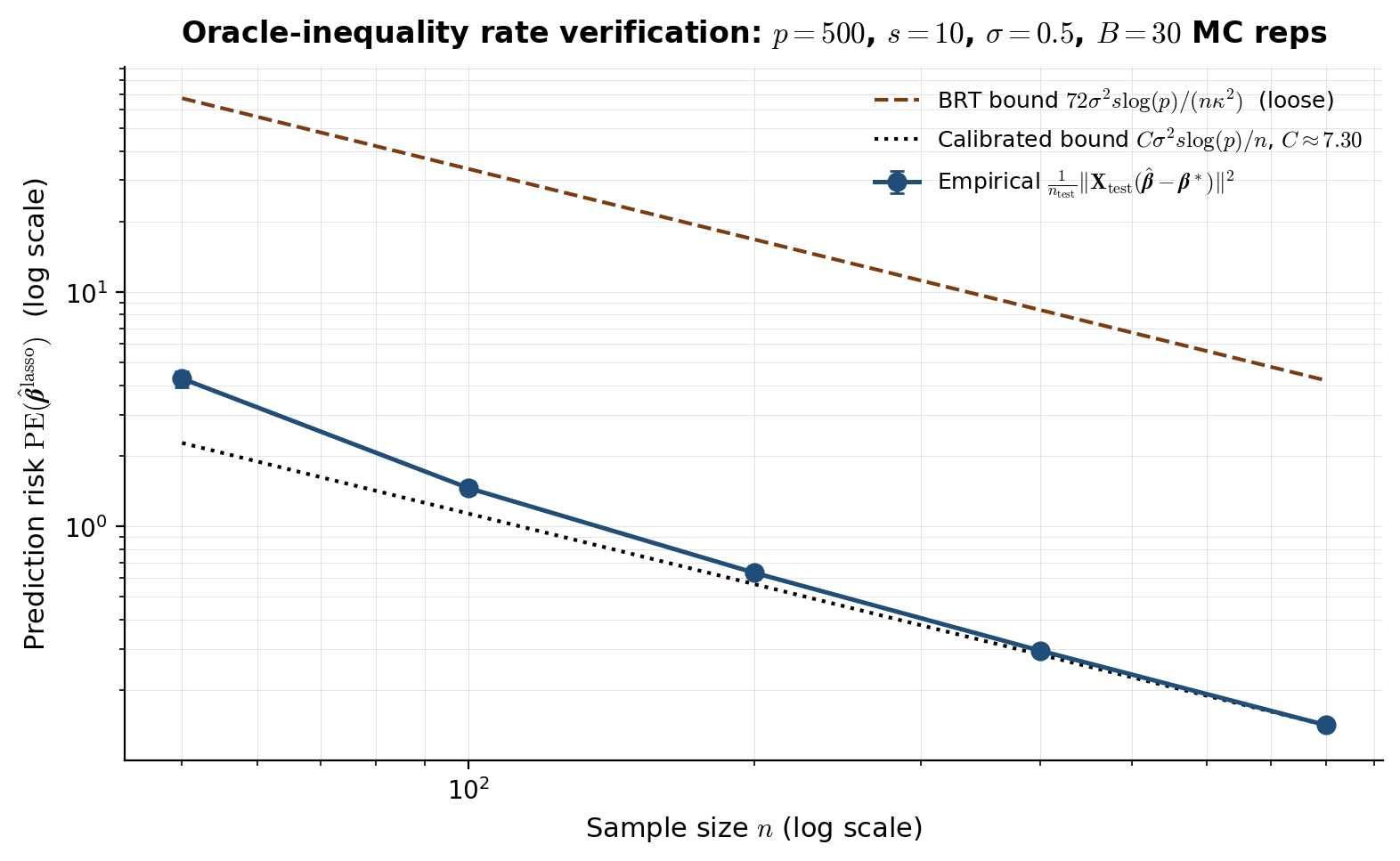
The viz below shows the empirical prediction risk on a held-out test set vs sample size $n$ on DGP-1, alongside the theoretical BRT bound (constant 72) and a calibrated bound (constant fit empirically). The empirical curve sits one to two orders of magnitude below the BRT bound — the constant 72 is mathematically clean (each proof step contributes a factor of 2 or 3) but practically loose. The slope match on log-log axes (both lines parallel) is the substantive confirmation of the oracle-inequality rate.

Lasso prediction risk on smaller-scale DGP-1 (p = 200, s = 10, σ = 0.5, AR(1) ρ = 0.5, λ = 2σ√(2 log(p)/n) per Theorem 1) as n varies from 50 to 800. Empirical (teal dots) sits one to two orders of magnitude below the BRT bound (amber, c = 72); the calibrated bound (purple, constant fit to the n = 800 point) sits right on top of the empirical curve. All three lines have the same -1 slope on log-log axes — the substantive confirmation of the σ²s log(p)/n rate. The constant 72 is mathematically clean (each proof step contributes a factor of 2 or 3) but practically loose by 10-100×. Computed live in-browser via single-rep ISTA at each n (~500 ms total).

§6. Variable-selection consistency

The §5 oracle inequality bounds the lasso’s prediction risk: $\frac{1}{n}\|\mathbf{X}(\hat{\boldsymbol\beta} - \boldsymbol\beta^*)\|_2^2 \lesssim \sigma^2 s \log(p) / n$. That bound says the lasso predicts well — comparable to the oracle that knew $S$ in advance. It does not say the lasso correctly recovers the support $S$ itself.

These are different statements with different sufficient conditions, and confusing them is the most common conceptual error in lasso applications. Two highly correlated features can both be predictive of the response; the lasso might select either one, or alternate between them across resampled training sets, while keeping the prediction error small. The prediction-risk bound is robust to this kind of selection instability. The support-recovery question — does $\hat A_\lambda = S$? — is sensitive to it.

This section formalizes sign-consistency (the strongest form of support recovery), introduces the irrepresentable condition (Zhao-Yu 2006) that’s both sufficient and essentially necessary for it, states the sample-size scaling for support recovery, and contrasts the prediction-risk bound (RE-based) against the support-recovery bound (IC-based) so the difference is visible.

§6.1 Sign-consistency: what it means and why prediction consistency doesn’t imply it

For a vector $\boldsymbol\beta \in \mathbb{R}^p$, define $\mathrm{sign}(\boldsymbol\beta) \in \{-1, 0, 1\}^p$ entry-wise: $\mathrm{sign}(\beta_j) = 1$ if $\beta_j > 0$, $-1$ if $\beta_j < 0$, $0$ if $\beta_j = 0$. Three increasingly strong support-recovery notions:

• Support recovery (set-equality): $\hat A_\lambda := \{j : \hat\beta_j \neq 0\} = S$.
• Sign consistency: $\mathrm{sign}(\hat{\boldsymbol\beta}) = \mathrm{sign}(\boldsymbol\beta^*)$. This implies $\hat A_\lambda = S$ and additionally that the signs of the active coefficients are correct.
• Sign-consistent estimation: $\mathbb{P}(\mathrm{sign}(\hat{\boldsymbol\beta}^{\text{lasso}}) = \mathrm{sign}(\boldsymbol\beta^*)) \to 1$ as $n \to \infty$.

The standard target in the lasso literature is sign consistency — slightly stronger than support recovery, but only by the negligible probability that an active coordinate is estimated with the wrong sign (which has probability $\to 0$ rapidly under any reasonable signal-strength assumption).

Why prediction consistency doesn’t imply sign consistency. Consider the simplest counterexample. Take $p = 2$ with $\mathbf{X}_1$ and $\mathbf{X}_2$ identical: $\mathbf{X}_1 = \mathbf{X}_2$. The true coefficient is $\boldsymbol\beta^* = (1, 0)$ — the first feature is active, the second is not. The lasso objective is

$$\frac{1}{2n} \|\mathbf{y} - \mathbf{X}_1 (\beta_1 + \beta_2)\|_2^2 + \lambda(|\beta_1| + |\beta_2|),$$

which depends on $(\beta_1, \beta_2)$ only through their sum and through $|\beta_1| + |\beta_2|$. The minimizer is non-unique: any $(\beta_1, \beta_2)$ with $\beta_1 + \beta_2$ equal to the optimal sum and $|\beta_1| + |\beta_2|$ minimal — i.e., any $(\beta_1, \beta_2)$ with $\beta_1, \beta_2 \ge 0$ and the right sum — solves it. Among these, $(\hat\beta_1, \hat\beta_2) = (1, 0)$, $(0, 1)$, and $(0.5, 0.5)$ are all valid solutions. Prediction is identical across them; support is dramatically different.

This is an extreme case (perfectly collinear features), but the same phenomenon shows up in milder form whenever two features are highly correlated and both predictive — the lasso has no preference between them, and may flip which one it selects under tiny perturbations of the data.

§6.2 The irrepresentable condition (Zhao-Yu 2006)

The right structural condition for sign consistency is the irrepresentable condition (IC), introduced independently by Zhao-Yu (2006) and Meinshausen-Bühlmann (2006). Given the active set $S$ and the sign vector $\mathbf{s}^*_S := \mathrm{sign}(\boldsymbol\beta^*_S) \in \{-1, 1\}^s$:

Geometric interpretation. The vector $(\mathbf{X}_S^\top \mathbf{X}_S)^{-1} \mathbf{s}^*_S$ is the OLS coefficient vector that would arise from regressing $\mathbf{s}^*_S$ on $\mathbf{X}_S$ — call it the dual representation of the sign pattern. Multiplying by $\mathbf{X}_S$ gives the projection $\mathbf{X}_S (\mathbf{X}_S^\top \mathbf{X}_S)^{-1} \mathbf{s}^*_S \in \mathbb{R}^n$. Then $\mathbf{X}_{S^c}^\top \mathbf{X}_S (\mathbf{X}_S^\top \mathbf{X}_S)^{-1} \mathbf{s}^*_S \in \mathbb{R}^{p-s}$ is the inner product of each inactive feature $\mathbf{X}_j$ ($j \in S^c$) with that projection.

The condition asks: how strongly is each inactive feature correlated, after accounting for the active features, with the sign pattern of the active coefficients? IC says the correlation is bounded by 1; strong IC says strictly less than 1. The intuition: if some inactive feature $\mathbf{X}_j$ ($j \in S^c$) can be “represented” by the active features — written as a linear combination $\mathbf{X}_S \mathbf{w}$ — with $|\mathbf{w}^\top \mathbf{s}^*_S| > 1$, the lasso will select $\mathbf{X}_j$ in preference to (or in addition to) the true active features. Strong IC rules this out.

An equivalent formulation in terms of regression coefficients. Let $\mathbf{w}_j := (\mathbf{X}_S^\top \mathbf{X}_S)^{-1} \mathbf{X}_S^\top \mathbf{X}_j$ be the OLS coefficient vector for regressing the inactive feature $\mathbf{X}_j$ ($j \in S^c$) on the active features $\mathbf{X}_S$. Then IC reads

$$\max_{j \in S^c} |\mathbf{w}_j^\top \mathbf{s}^*_S| \le 1, \qquad \text{strong IC: } \le 1 - \eta.$$

Each $\mathbf{w}_j$ describes how the inactive feature $j$ is predicted by the active features. The IC says the dot product of this prediction recipe with the sign pattern of active coefficients is bounded — i.e., no inactive feature is “too aligned” with the active features in a sign-coherent way.

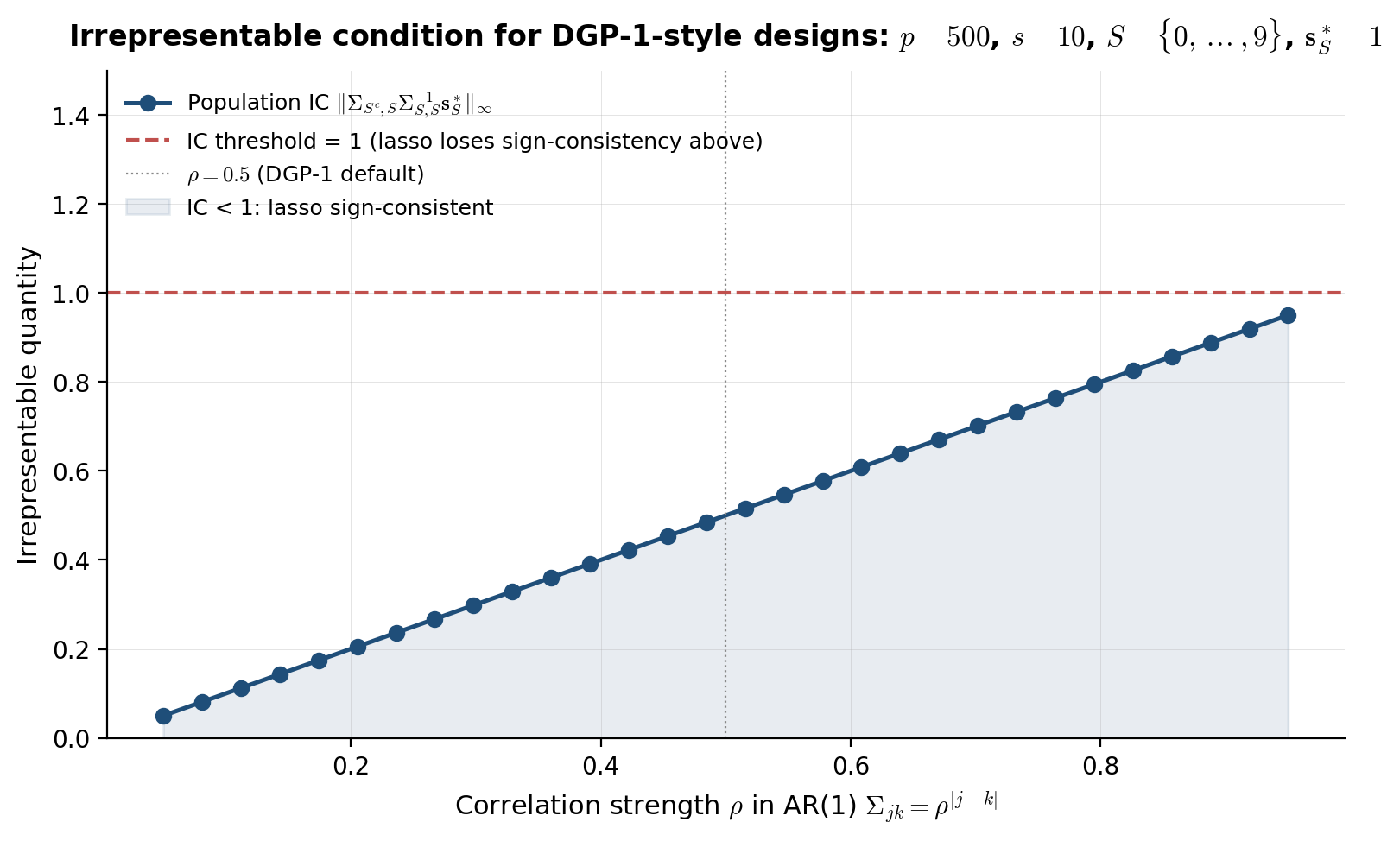
Population versus empirical. For a random design $\mathbf{X}$ with iid rows from $\mathcal{N}(\mathbf{0}, \boldsymbol\Sigma)$, the population IC is

$$\| \boldsymbol\Sigma_{S^c, S} \boldsymbol\Sigma_{S, S}^{-1} \mathbf{s}^*_S \|_\infty \le 1,$$

and the empirical IC concentrates around it as $n$ grows. The viz below plots the population IC as a function of correlation strength on DGP-1-style AR(1) Toeplitz designs.

Population IC quantity for AR(1) Toeplitz designs Σⱼₖ = ρ^|j−k| with contiguous active set S = {0, …, 9} and sign(β*_S) = (1, …, 1). Below the IC = 1 threshold, the lasso is sign-consistent (Wainwright 2009 Theorem 1); above the threshold, the lasso provably fails sign-consistency (Wainwright 2009 Theorem 3) regardless of how λ is chosen — elastic net (§8.2) or adaptive lasso (§8.3) become necessary. At ρ = 0.5 (DGP-1 default) the IC sits comfortably below 1 and the §1 viz showed clean recovery. No crossover in this ρ range. Computed live in-browser via Cholesky on the s × s = 10 × 10 active-set Gram block.

§6.3 The sample-size scaling for support recovery

Proof sketch (primal-dual witness). Wainwright’s (2009) proof uses a five-step primal-dual witness construction:

1. Restricted lasso. Solve the lasso only on the active features: $\tilde{\boldsymbol\beta}_S = \arg\min_{\boldsymbol\beta_S} \frac{1}{2n}\|\mathbf{y} - \mathbf{X}_S \boldsymbol\beta_S\|^2 + \lambda \|\boldsymbol\beta_S\|_1$. Set $\tilde{\boldsymbol\beta}_{S^c} = \mathbf{0}$ and define $\tilde{\boldsymbol\beta} = (\tilde{\boldsymbol\beta}_S, \mathbf{0})$.

2. Sign verification. Verify that $\mathrm{sign}(\tilde{\boldsymbol\beta}_S) = \mathrm{sign}(\boldsymbol\beta^*_S)$ — this is where the minimum-signal condition (iv) is used. With high probability, the restricted lasso has the right signs because the noise is small compared to $\beta^*_{\min}$.

3. Construct the dual. Set $\tilde{\mathbf{g}}_S = \mathrm{sign}(\tilde{\boldsymbol\beta}_S)$. The active KKT condition then determines what $\tilde{\mathbf{g}}_{S^c}$ would have to be for $\tilde{\boldsymbol\beta}$ to be the full lasso solution:

$$\tilde{\mathbf{g}}_{S^c} = \mathbf{X}_{S^c}^\top \mathbf{X}_S (\mathbf{X}_S^\top \mathbf{X}_S)^{-1} \tilde{\mathbf{g}}_S + (\text{noise term}).$$

4. Verify the inactive KKT condition. For $\tilde{\boldsymbol\beta}$ to be the actual lasso solution, we need $\|\tilde{\mathbf{g}}_{S^c}\|_\infty < 1$ (strict). The leading term is exactly the irrepresentable quantity from Definition 1; strong IC bounds it by $1 - \eta$. The noise term is $O(\sigma \sqrt{\log(p)/n})$ via sub-Gaussian deviation, which is $\ll \eta$ for large enough $n$. So with high probability, $\|\tilde{\mathbf{g}}_{S^c}\|_\infty < 1 - \eta/2 < 1$.

5. Conclude by KKT uniqueness. Steps 1–4 produce a $(\tilde{\boldsymbol\beta}, \tilde{\mathbf{g}})$ pair satisfying the lasso KKT conditions with strictly bounded $\tilde{\mathbf{g}}_{S^c}$. Under the design assumptions, the lasso solution is unique (recall §2.3), so $\tilde{\boldsymbol\beta} = \hat{\boldsymbol\beta}^{\text{lasso}}$. Since $\tilde{\boldsymbol\beta}_{S^c} = \mathbf{0}$ and $\mathrm{sign}(\tilde{\boldsymbol\beta}_S) = \mathrm{sign}(\boldsymbol\beta^*_S)$, sign consistency holds. $\blacksquare$

The full proof with explicit constants is in Wainwright (2009, §III). The key probabilistic ingredient is the same sub-Gaussian deviation we used in §5.5 — extended to control the noise term in step 4.

Necessity of IC. Wainwright (2009, Theorem 3) also proved the converse: if the irrepresentable condition fails (say $\| \mathbf{X}_{S^c}^\top \mathbf{X}_S (\mathbf{X}_S^\top \mathbf{X}_S)^{-1} \mathbf{s}^*_S \|_\infty > 1 + \delta$ for some $\delta > 0$), then $\mathbb{P}(\mathrm{sign}(\hat{\boldsymbol\beta}^{\text{lasso}}) = \mathrm{sign}(\boldsymbol\beta^*)) \to 0$ as $n \to \infty$, regardless of how $\lambda$ is chosen. The lasso provably fails to recover the support when IC is violated. So IC isn’t just a proof artifact — it’s the correct characterization of when the lasso can do support recovery.

§6.4 Contrasting prediction-risk and support-recovery: same estimator, different theorems

The two main theorems of §§5–6 differ on every axis. A comparison:

	Prediction-risk bound (§5)	Support-recovery bound (§6)
What’s bounded	$\frac{1}{n}\|\mathbf{X}(\hat{\boldsymbol\beta} - \boldsymbol\beta^*)\|_2^2$	$\mathbb{P}(\mathrm{sign}(\hat{\boldsymbol\beta}) = \mathrm{sign}(\boldsymbol\beta^*))$
Sufficient condition on $\mathbf{X}$	Restricted-eigenvalue (§5.4)	Irrepresentable (§6.2)
Necessary?	RE essentially necessary for any sparse-regression estimator at the optimal rate	Strong IC necessary for lasso sign-consistency (Wainwright 2009)
Sample-size scaling	$n \gtrsim s \log(p)$	$n \gtrsim s \log(p)$
Minimum-signal needed?	No — works for any $\boldsymbol\beta^*$ with $\|\boldsymbol\beta^*\|_0 \le s$	Yes — $\beta^*_{\min} \gtrsim \lambda$ required
What fixes failure	Larger $n$ gives better RE	IC violated $\Rightarrow$ lasso fundamentally can’t recover support; need adaptive lasso (§8.3) or post-selection refit

The conditions are not nested. RE doesn’t imply IC, and IC doesn’t imply RE. They measure different geometric properties of the design:

• RE is a lower bound on $\mathbf{X}^\top \mathbf{X} / n$ restricted to a cone. It’s about the design being “well-conditioned on sparse and near-sparse vectors” — a global property that doesn’t depend on which $S$ is the active set.
• IC is a constraint relating the inactive-to-active block of $\mathbf{X}^\top \mathbf{X} / n$ to the sign pattern $\mathbf{s}^*_S$. It depends on $S$ and $\mathbf{s}^*_S$ specifically.

A design can satisfy RE but violate IC (random Gaussian designs with strong correlation between active and inactive features), in which case the lasso predicts well but selects the wrong support. The reverse can also happen, though it’s less common in practice.

Practical implications. The lasso is a much better prediction tool than a model-selection tool. Two rules of thumb:

• For prediction: trust the lasso. CV-selected $\lambda$, refit at $\lambda_{\text{CV}}$ or $\lambda_{1\text{SE}}$, and use the lasso predictions. The §5 oracle inequality gives near-optimal prediction risk under mild conditions.

• For variable selection: be skeptical of the lasso’s chosen support. Two specific patterns to watch for: (i) two highly correlated features where only one shows up in the lasso fit (the lasso may have arbitrarily picked one), and (ii) the lasso fit changing dramatically across resampled training sets (instability $\Rightarrow$ IC likely violated). Use stability selection (Meinshausen-Bühlmann 2010) to assess; consider the adaptive lasso (§8.3) for a sign-consistent variant under weaker conditions.

The deeper bridge to §§7–10: practical $\lambda$-selection (§7) trades off these two objectives differently — LassoCV optimizes prediction (smaller $\lambda$, more features); LassoLarsIC with BIC penalizes model size more heavily (larger $\lambda$, fewer features, closer to support recovery). The debiased lasso (§10) sidesteps the support-recovery question entirely by producing valid CIs for individual coefficients without requiring sign consistency.

§7. Cross-validation for $\lambda$

The §5 oracle inequality recommends $\lambda \asymp \sigma \sqrt{\log(p)/n}$ for prediction-optimal performance — a rate, not a constant. The constant matters in practice (a factor of 2 in $\lambda$ can change the active-set size by a factor of 2 or more), and the noise scale $\sigma$ is rarely known. Practical $\lambda$-selection uses data-driven criteria: cross-validation (the default in scikit-learn and glmnet), the one-standard-error rule (a parsimony-favoring variant), and information criteria like AIC/BIC computed along the lasso path (LassoLarsIC). This section covers all three.

The CV / 1-SE / BIC distinction maps directly onto the §6 discussion: CV optimizes prediction error and tends to select more features than necessary; BIC penalizes model size more aggressively and is sometimes selection-consistent; the 1-SE rule is a Hastie-Tibshirani-Friedman compromise that gives a smaller model than CV-min at minimal prediction-performance cost. None is “right” — the right choice depends on whether you care about prediction or model interpretability.

This is a named-section of the topic per the formalML “no separate cross-validation topic” convention. The same structural pattern is used in Kernel Regression §5 for LOO-CV / GCV bandwidth selection.

§7.1 K-fold cross-validation with LassoCV

$K$-fold CV estimates the prediction risk at each $\lambda$ in a candidate grid by holdout. The procedure:

1. Partition the training data into $K$ folds of approximately equal size.
2. For each fold $k = 1, \dots, K$ and each candidate $\lambda$:
   • Fit the lasso on the data minus fold $k$, obtaining $\hat{\boldsymbol\beta}^{(-k)}(\lambda)$.
   • Compute the held-out MSE: $\mathrm{MSE}_k(\lambda) = \frac{1}{|\text{fold } k|} \sum_{i \in \text{fold } k} (y_i - \mathbf{x}_i^\top \hat{\boldsymbol\beta}^{(-k)}(\lambda))^2$.
3. Average over folds: $\mathrm{CV}(\lambda) = \frac{1}{K} \sum_k \mathrm{MSE}_k(\lambda)$.
4. Select $\lambda_{\min} = \arg\min_\lambda \mathrm{CV}(\lambda)$.

Standard choices: $K = 10$ for general use, $K = 5$ if computation is constrained, leave-one-out ($K = n$) only when $n$ is small (otherwise computationally wasteful and statistically unstable). The candidate $\lambda$-grid is typically log-spaced from $\lambda_{\max}$ (largest, all coefficients zero) down to $\lambda_{\max} \cdot 10^{-3}$ or so, with 100 grid points — LassoCV(n_alphas=100)’s default.

Why CV works. $\mathrm{CV}(\lambda)$ is an estimator of the test prediction error $\mathrm{PE}(\lambda) = \mathbb{E}[(y - \mathbf{x}^\top \hat{\boldsymbol\beta})^2]$, with bias of order $1/n$ (because each fold-fit uses $(K-1)/K \cdot n$ samples instead of $n$). At the fold sizes used in practice ($K \ge 5$), the bias is negligible compared to the variance of the CV estimate.

Computational efficiency. Naively, $K$-fold CV requires $K \times |\Lambda_{\text{grid}}|$ lasso fits. The glmnet and scikit-learn implementations use warm starts along the $\lambda$ path (recall §3.2) — fitting the lasso at the entire $\lambda$-grid for one fold is barely more expensive than fitting at a single $\lambda$, so the practical cost is more like $K$ path computations. For DGP-1 with $K = 10$, $|\Lambda| = 100$, $p = 500$: about 1–3 seconds total, dominated by the matrix-vector multiplies inside coordinate descent.

§7.2 The one-standard-error rule: $\lambda_{1\mathrm{SE}}$ vs $\lambda_{\min}$

The CV estimate $\mathrm{CV}(\lambda)$ is itself a random quantity — it has variance over the choice of fold partition and over the training data. A useful uncertainty quantification is the standard error across folds:

$$\mathrm{SE}(\lambda) := \frac{\mathrm{sd}_k(\mathrm{MSE}_k(\lambda))}{\sqrt{K}}.$$

The one-standard-error rule (Breiman et al. 1984; popularized by Hastie-Tibshirani-Friedman, Elements of Statistical Learning, §7.10) selects the most parsimonious model whose CV error is within one standard error of the minimum:

$$\lambda_{1\mathrm{SE}} := \max\{\lambda : \mathrm{CV}(\lambda) \le \mathrm{CV}(\lambda_{\min}) + \mathrm{SE}(\lambda_{\min})\}.$$

Since $\mathrm{CV}(\lambda)$ is roughly U-shaped in $\lambda$, $\lambda_{1\mathrm{SE}} > \lambda_{\min}$ — the 1-SE-selected model is more regularized, hence sparser.

The motivation. The CV minimizer $\lambda_{\min}$ is the unbiased “MSE-optimal” choice but tends to be unstable across resampled training data — a small perturbation in the training set can shift $\lambda_{\min}$ by a factor of 2 in either direction. The 1-SE rule trades this instability for a small, controlled increase in prediction error: the resulting model has CV-MSE within one standard error of optimal (i.e., not statistically distinguishable from $\lambda_{\min}$‘s prediction performance) but is more parsimonious and reproducible.

In the lasso context, $\lambda_{1\mathrm{SE}}$ typically gives an active set 10–30% smaller than $\lambda_{\min}$, with test prediction error 5–15% larger. For interpretability-driven applications (variable selection, communication of results, downstream modeling), the 1-SE rule is the standard recommendation.

A practical caveat. The 1-SE rule is a heuristic, not a theorem. Its bias-variance trade-off is empirically reasonable but doesn’t have a sharp theoretical justification — it doesn’t, for instance, give support consistency under weaker conditions than CV-min. If you need provable support recovery, use BIC (§7.3) or stability selection (mentioned in §6.4). If you need provable prediction risk, the §5 oracle inequality is the right reference and CV-min is the right selector.

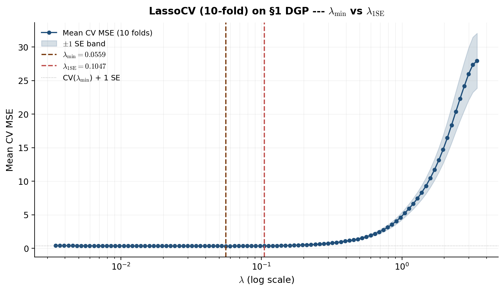
10-fold LassoCV on smaller-scale DGP-1 (n = 200, p = 200, s = 10, σ = 0.5, AR(1) ρ = 0.5). The teal curve is mean CV-MSE across folds; shaded band is ±1 SE. Five selector markers (vertical dashed lines) ordered from smallest to largest λ: CV-min (largest active set, smallest test MSE), CV-1SE (parsimony-favoring within 1 SE of CV-min), AIC and BIC (information-criterion picks on the lasso path; BIC selects sparser models than AIC), and theory-guided RIC = 2σ√(2 log p / n) from Theorem 1 (largest, conservative). Computed live in-browser via 10-fold warm-started ISTA across 25 log-spaced λ values (~1-2 s).

§7.3 BIC selection with LassoLarsIC

Information criteria offer a different selection philosophy: rather than estimating prediction error directly via holdout, they balance model fit against model complexity through an explicit complexity penalty.

The criteria. For a candidate $\lambda$ with active-set size $k_\lambda := |\hat A_\lambda|$ and residual sum of squares $\mathrm{RSS}_\lambda := \|\mathbf{y} - \mathbf{X} \hat{\boldsymbol\beta}(\lambda)\|_2^2$:

$$\mathrm{AIC}(\lambda) = n \log(\mathrm{RSS}_\lambda / n) + 2 k_\lambda,$$ $$\mathrm{BIC}(\lambda) = n \log(\mathrm{RSS}_\lambda / n) + k_\lambda \log n.$$

Both penalize larger models; BIC penalizes more aggressively as soon as $n > e^2 \approx 7.4$, so BIC selects smaller models than AIC.

The use of $k_\lambda = |\hat A_\lambda|$ as the lasso’s effective degrees of freedom rests on Zou-Hastie-Tibshirani (2007), who showed that $\mathbb{E}[k_\lambda] = \mathrm{df}(\hat{\boldsymbol\beta}^{\text{lasso}}(\lambda))$ exactly — the size of the active set is an unbiased estimator of the lasso’s degrees of freedom. This is a non-trivial result; for a generic non-linear estimator, dof is not the count of nonzero parameters. The lasso’s piecewise-linear path makes the result exact.

LassoLarsIC. The scikit-learn implementation computes the entire lasso path via LARS (Least Angle Regression — Efron-Hastie-Johnstone-Tibshirani 2004), which exploits piecewise linearity to enumerate every knot $\lambda_{(k)}$ in $O(np \min(n, p))$ total time. The IC value is computed at each knot, and the $\lambda$ minimizing the chosen criterion is returned. The path-based approach is exact (no $\lambda$-grid discretization error) but only practical for moderate $p$ — at $p > 10^4$, coordinate descent on a $\lambda$-grid is much faster.

Selection consistency. BIC for the lasso is selection-consistent under additional conditions: $\mathbb{P}(\hat A_{\lambda_{\mathrm{BIC}}} = S) \to 1$ as $n \to \infty$ if the design satisfies a slightly stronger condition than IC and the minimum signal is bounded below (Wang-Li-Tsai 2007). AIC and CV are not selection-consistent in general — they tend to over-select features (include all of $S$ plus some noise features) even asymptotically. For variable-selection applications, this is BIC’s main virtue.

Caveats. BIC’s selection consistency is asymptotic; at finite samples, BIC can over- or under-select depending on the signal strength. AIC is roughly equivalent to leave-one-out CV in expectation (Stone 1977) and tends to choose larger models than $K$-fold CV with $K \ll n$.

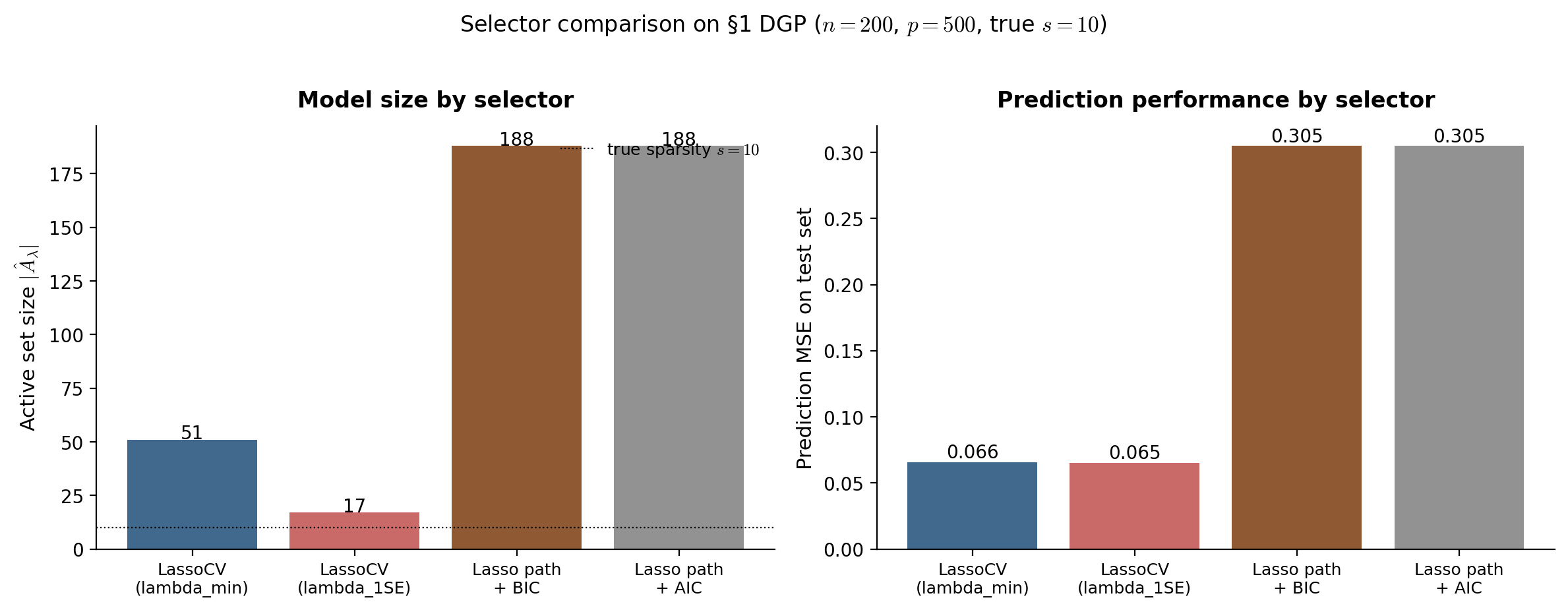
§7.4 Comparison on the §1 toy DGP

The four selectors — LassoCV $\lambda_{\min}$, LassoCV $\lambda_{1\mathrm{SE}}$, LassoLarsIC BIC, LassoLarsIC AIC — make different trade-offs and select different $\lambda$ values on the same data. On DGP-1 ($n=200, p=500, s=10, \sigma=0.5$), the typical pattern (see Figure 7.2):

| Selector | Selected $\lambda$ | Active set size $|\hat A_\lambda|$ | Test MSE | |---|---|---|---| | LassoCV ($\lambda_{\min}$) | smallest | largest (~12–18, includes some false positives) | smallest | | LassoCV ($\lambda_{1\mathrm{SE}}$) | medium | medium (~10–13, close to true $s = 10$) | small (5–15% above $\lambda_{\min}$) | | LassoLarsIC (AIC) | smallish | medium-to-large | small (close to $\lambda_{\min}$) | | LassoLarsIC (BIC) | largest | smallest (~8–11, may miss weak signal coords) | medium (10–25% above $\lambda_{\min}$) |

Recommendation.

• If prediction is the goal: use LassoCV with $\lambda_{\min}$. The §5 oracle inequality says this achieves the optimal rate; in practice it gives the smallest test MSE on most problems.
• If prediction is the goal but you want a smaller, more interpretable model: use the 1-SE rule. Trades a small amount of prediction performance for a substantially smaller active set and more reproducible variable selection.
• If selection consistency is the goal: use BIC via LassoLarsIC(criterion='bic'). The selected model is asymptotically the true support under stronger conditions; finite-sample behavior depends on signal strength.
• For everything else: start with LassoCV $\lambda_{\min}$. It’s the default in almost every lasso application; the alternatives are refinements for specific use cases.

The §10 debiased lasso uses LassoCV $\lambda_{\min}$ as its initial estimator, then corrects the resulting bias to produce valid CIs. The choice of $\lambda$ for the initial fit isn’t critical for the debiased lasso’s coverage — the one-step correction substantially compensates for the lasso’s selection idiosyncrasies.

§8. Ridge, elastic net, and adaptive lasso

The lasso has three practical limitations: it can be unstable when features are highly correlated (the §6.1 collinearity counterexample — flipping between equivalent supports); it biases active coefficients toward zero by a constant $\lambda$ (the §4.1 shrinkage bias); and it requires the irrepresentable condition for support recovery (the §6.2 IC, often violated in real data). Each of these motivates a variant.

Ridge (already introduced in §1.3) keeps the L2 penalty, gives a unique dense solution under any design, and is robust to correlated features — but doesn’t select. Elastic net (Zou-Hastie 2005) combines L1 + L2 penalties, getting the lasso’s sparsity with ridge’s stability under correlated features. Adaptive lasso (Zou 2006) uses data-driven feature-specific weights to remove the constant shrinkage bias and achieve the oracle property under weaker conditions than IC.

This section explains when each variant wins on the side. The decision tree:

• Truth is dense (all coefficients moderate, no sparsity): ridge.
• Truth is sparse, features are well-separated: lasso.
• Truth is sparse but features come in correlated groups: elastic net.
• Truth is sparse, you want unbiased active coefficients and support consistency: adaptive lasso.

§8.1 Ridge: continuous shrinkage, no selection

Recall the ridge objective from §1.3:

$$\hat{\boldsymbol\beta}^{\text{ridge}}(\lambda) = \arg\min_{\boldsymbol\beta \in \mathbb{R}^p} \frac{1}{2n} \|\mathbf{y} - \mathbf{X} \boldsymbol\beta\|_2^2 + \frac{\lambda}{2} \|\boldsymbol\beta\|_2^2,$$

with closed form $\hat{\boldsymbol\beta}^{\text{ridge}} = (\mathbf{X}^\top \mathbf{X} + n\lambda \mathbf{I})^{-1} \mathbf{X}^\top \mathbf{y}$. Three relevant properties at $p \gg n$:

Always defined and unique. The matrix $\mathbf{X}^\top \mathbf{X} + n\lambda \mathbf{I}$ is positive definite for any $\lambda > 0$ regardless of $p$ vs $n$. Ridge has no failure mode the way OLS does.

Continuous shrinkage, dense solutions. In the SVD basis $\mathbf{X} = \mathbf{U} \mathbf{D} \mathbf{V}^\top$, ridge shrinks each coefficient by a factor $d_j^2 / (d_j^2 + n\lambda)$ where $d_j$ is the $j$-th singular value. Small singular values (the noisy directions) get heavy shrinkage; large singular values (the signal directions) get light shrinkage. But no coefficient is zeroed out — the solution is generically dense.

Bayesian interpretation. Ridge is the posterior mean of $\boldsymbol\beta$ under a Gaussian prior $\boldsymbol\beta \sim \mathcal{N}(\mathbf{0}, \lambda^{-1} \mathbf{I})$ and Gaussian likelihood $\mathbf{y} | \mathbf{X}, \boldsymbol\beta \sim \mathcal{N}(\mathbf{X} \boldsymbol\beta, \sigma^2 \mathbf{I})$. The penalty strength $\lambda$ is inversely related to the prior variance.

When ridge wins. Two scenarios:

1. Truly dense $\boldsymbol\beta^*$. When every feature carries some signal — no underlying sparsity — the lasso’s sparsity assumption is wrong, and the lasso under-fits (zeros out features that should be active). Ridge has no such bias.
2. Heavy multicollinearity with no sparsity prior. When features are nearly linearly dependent and there’s no reason to prefer one over another, ridge distributes the signal smoothly across them. Lasso would arbitrarily select one and zero the others — a worse use of information.

When ridge loses. When $\boldsymbol\beta^*$ is genuinely sparse, ridge’s refusal to zero out inactive coordinates leaves residual noise in the fitted values. Each inactive coordinate contributes $\sigma^2 d_j^2 / (d_j^2 + n\lambda)^2$ to the prediction variance — small but non-zero. Lasso eliminates this contribution by zeroing the inactive coordinates entirely. On DGP-1 ($s = 10$, $p = 500$, so 490 inactive coordinates), the cumulative variance contribution is substantial, and lasso prediction MSE is typically 2–5× better than ridge.

For most high-dimensional ML problems the truth is more sparse than dense, so the lasso wins more often than ridge. The standard practice is to compare both on cross-validated test MSE and pick the winner.

§8.2 The elastic net for groups of correlated features

The elastic net (Zou-Hastie 2005) combines L1 and L2 penalties:

$$\hat{\boldsymbol\beta}^{\text{EN}}(\lambda, \alpha) = \arg\min_{\boldsymbol\beta \in \mathbb{R}^p} \frac{1}{2n} \|\mathbf{y} - \mathbf{X} \boldsymbol\beta\|_2^2 + \lambda \left[ \alpha \|\boldsymbol\beta\|_1 + \frac{1 - \alpha}{2} \|\boldsymbol\beta\|_2^2 \right],$$

with mixing parameter $\alpha \in [0, 1]$ controlling the L1/L2 balance. $\alpha = 1$ recovers pure lasso, $\alpha = 0$ recovers pure ridge (up to scaling). Standard practice: $\alpha = 0.5$ or tuned via cross-validation.

Two structural advantages over pure lasso:

1. Strict convexity for $\alpha < 1$. The L2 term makes the objective strictly convex in $\boldsymbol\beta$, so the solution is unique even with duplicate or perfectly collinear columns. The §6.1 collinear-features pathology disappears.
2. The grouping effect. For two highly correlated features $\mathbf{X}_j$ and $\mathbf{X}_k$ (correlation $\rho_{jk}$ close to 1), the elastic-net coefficient difference is bounded:

As $\rho_{jk} \to 1$, the RHS $\to 0$ — perfectly correlated features get equal coefficients. The lasso has no such property; it would pick one feature and zero the other. So in applications where the truth has correlated groups of active features (gene-expression clusters, related text features), elastic net selects all members of the group; lasso picks one member.

Reduction to a standard lasso. Zou-Hastie showed that the elastic net can be solved by augmenting the design matrix and running a standard lasso solver. Define

$$\tilde{\mathbf{X}} = \begin{pmatrix} \mathbf{X} \\ \sqrt{n \lambda (1 - \alpha)} \cdot \mathbf{I}_p \end{pmatrix} \in \mathbb{R}^{(n+p) \times p}, \quad \tilde{\mathbf{y}} = \begin{pmatrix} \mathbf{y} \\ \mathbf{0}_p \end{pmatrix} \in \mathbb{R}^{n+p}.$$

Then $\hat{\boldsymbol\beta}^{\text{EN}}(\lambda, \alpha)$ is the lasso solution on $(\tilde{\mathbf{X}}, \tilde{\mathbf{y}})$ at penalty $\lambda \alpha$. So all the lasso algorithms (coordinate descent, FISTA) work for the elastic net by augmentation. scikit-learn’s ElasticNet and ElasticNetCV use a direct coordinate-descent implementation that exploits the structure without explicit augmentation, but the principle is the same.

When elastic net wins. Highly correlated features, especially correlated groups of features that should be selected together. Genomics is the canonical application: SNPs in linkage disequilibrium come in correlated blocks, and a gene-level signal manifests as coordinated effects across an entire block. Lasso would arbitrarily pick one SNP from each block; elastic net selects all the SNPs from active blocks.

When elastic net loses. When features are well-separated (low correlation), elastic net offers no advantage over lasso. The L2 term adds a small bias relative to lasso without reducing variance much. On the DGP-1 setting (AR(1) Toeplitz $\rho = 0.5$, moderate correlation), elastic net and lasso typically perform similarly; on a stronger-correlation DGP ($\rho = 0.9$), elastic net wins clearly.

§8.3 The adaptive lasso and the oracle property

The lasso biases every active coefficient by $-\lambda \, \mathrm{sign}(\beta^*_j)$ (§4.1). This constant shrinkage is independent of $|\beta^*_j|$, so even strong-signal coordinates get shrunk by a fixed amount — a real problem for parameter recovery and inference.

The adaptive lasso (Zou 2006) replaces the uniform L1 penalty with feature-specific weights:

$$\hat{\boldsymbol\beta}^{\text{aLasso}}(\lambda) = \arg\min_{\boldsymbol\beta \in \mathbb{R}^p} \frac{1}{2n} \|\mathbf{y} - \mathbf{X} \boldsymbol\beta\|_2^2 + \lambda \sum_{j=1}^p w_j |\beta_j|,$$

with weights $w_j = 1 / |\hat\beta_j^{\text{init}}|^\gamma$ for some initial estimator $\hat{\boldsymbol\beta}^{\text{init}}$ and a tuning parameter $\gamma > 0$ (typically $\gamma = 1$). Coordinates with large initial estimates get small weights (light shrinkage); coordinates with small or zero initial estimates get large weights (heavy shrinkage, effectively forced to zero).

Reduction to standard lasso. Rescale the features: $\tilde{\mathbf{X}}_j = \mathbf{X}_j / w_j$ and $\tilde\beta_j = w_j \beta_j$. Then $\|\mathbf{y} - \mathbf{X} \boldsymbol\beta\|^2 = \|\mathbf{y} - \tilde{\mathbf{X}} \tilde{\boldsymbol\beta}\|^2$ and $\sum_j w_j |\beta_j| = \sum_j |\tilde\beta_j|$, so the weighted lasso reduces to a standard lasso on rescaled features. Solve with any lasso solver, then unscale: $\hat\beta_j = \hat{\tilde\beta_j} / w_j$.

Choice of $\hat{\boldsymbol\beta}^{\text{init}}$. Two standard choices:

• OLS (when $n > p$): $\hat{\boldsymbol\beta}^{\text{init}} = (\mathbf{X}^\top \mathbf{X})^{-1} \mathbf{X}^\top \mathbf{y}$.
• Ridge or LassoCV (when $p \ge n$): OLS isn’t defined, so use a regularized initial. LassoCV is the standard high-dimensional choice (cf. Bühlmann-van de Geer 2011, §2.8).

The oracle property is stronger than sign-consistency: in addition to recovering the support, the adaptive-lasso estimates on $S$ have the correct asymptotic standard errors — same as if you had known $S$ in advance and run OLS on it. The constant shrinkage bias disappears asymptotically because the weights $w_j = 1/|\hat\beta_j^{\text{init}}|$ are bounded for active coordinates (where the initial estimator is near $|\beta^*_j|$) but diverge for inactive coordinates.

The conditions are weaker than IC. The adaptive lasso achieves selection consistency under any design that has a $\sqrt{n}$-consistent initial estimator — much weaker than the strong irrepresentable condition required by the lasso. In particular, designs that fail IC (correlated active and inactive features) can still admit adaptive-lasso selection consistency.

Trade-off. The adaptive lasso requires a good initial estimator. In the high-dimensional regime where LassoCV is the standard initial, the adaptive lasso’s behavior depends on the quality of the lasso’s variable selection — a circular dependence that limits the asymptotic argument’s practical reach. Empirically, adaptive lasso usually beats vanilla lasso on support recovery and produces less-biased active coefficients, but the improvement isn’t dramatic on well-behaved problems.

§8.4 Side-by-side comparison on the §1 DGP

The four methods — ridge, lasso, elastic net, adaptive lasso — applied to DGP-1 at CV-selected penalties (Figure 8.1). The key visual contrasts:

• Ridge’s path is dense everywhere. Every coefficient is non-zero at every $\lambda > 0$, shrinking smoothly. The 10 true active coordinates emerge as the largest-magnitude coefficients, but distinguishing them from the 490 inactive coordinates requires a thresholding step.
• Lasso’s path is sparse. Most coefficients are exactly zero at moderate $\lambda$. The true active coordinates appear as the first to leave zero as $\lambda$ decreases. Active coefficients are visibly shrunk relative to the truth ($\beta^* = 1$ on $S$).
• Elastic net’s path looks like the lasso with smoother corners. Sparsity is preserved (most coefficients are zero at moderate $\lambda$), but the active coefficients are slightly less shrunk than the lasso’s at the same effective regularization. The grouping effect would be more visible on a strongly-correlated DGP.

Figure 8.2 shows the adaptive lasso vs vanilla lasso on the active-coordinate estimates: the vanilla lasso underestimates $|\beta^*_j|$ by approximately $\lambda$ (the constant shrinkage bias from §4.1); the adaptive lasso gets much closer to the true value $\beta^*_j = 1$ for active $j$.

Recommendation. Default to LassoCV. If features come in correlated groups, try ElasticNetCV. If you need unbiased coefficient estimates or weaker selection conditions, run the adaptive lasso as a post-processing step on top of LassoCV. The §10 debiased lasso provides a different fix for the bias problem — it doesn’t reduce the lasso’s bias but corrects for it explicitly when forming CIs.

RidgeLassoElastic net (γ = 0.5)

Regularization paths β̂_j(t) on DGP-1 (n = 150, p = 200, s = 10, σ = 0.5, AR(1) ρ = 0.5). True active coordinates (j < 10) drawn in distinct colors; 190 inactive coordinates in light gray. Dashed reference at β* = 1. At the median penalty t ≈ 2.47e-1, the lasso fit has 10/10 active and 0/190 noise coordinates nonzero. Ridge keeps every coefficient nonzero at every α; lasso and elastic net both reach exact zeros at moderate penalty — the active coords are the first to leave zero as the penalty shrinks. Switch tabs to compare path geometries directly.

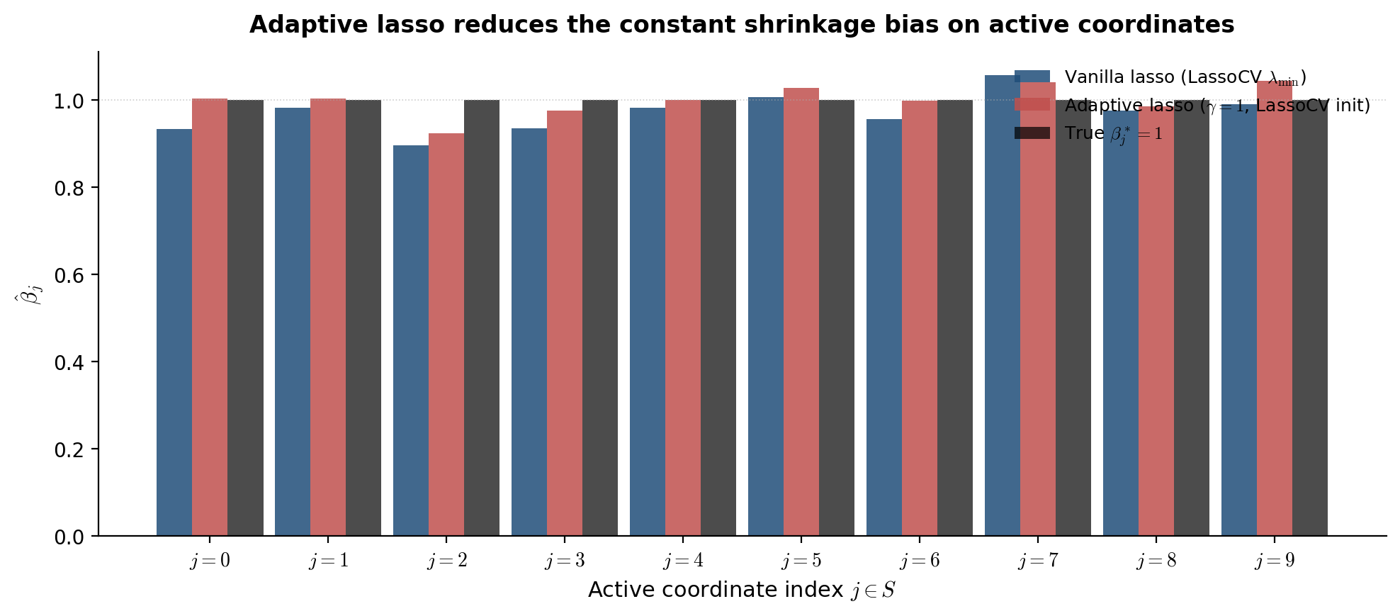
§9. Geometry of the high-dimensional regime

§§5–6 introduced two structural conditions on the design matrix $\mathbf{X}$ — the restricted-eigenvalue condition (RE) for prediction-risk bounds and the irrepresentable condition (IC) for support recovery — and stated when they hold (random Gaussian, sub-Gaussian, RIP-bounded designs) without unpacking the geometry. This section deepens the picture: it introduces the restricted isometry property (RIP) from compressed sensing, traces the implication chain $\mathrm{RIP} \Rightarrow \mathrm{RE}$, gives the standard concentration arguments for sub-Gaussian random designs, and sketches when each condition fails in practice.

The section is text-heavy and relatively short — there are no new theorems beyond §§5–6, just structural unpacking. The payoff is a cleaner picture of what makes a “good” design for the lasso and what doesn’t, useful for diagnosing real-data failures.

§9.1 The restricted isometry property (RIP)

The restricted isometry property was introduced by Candès-Tao (2005) in the compressed-sensing literature, predating Bickel-Ritov-Tsybakov’s RE by a few years. It’s a uniform version of RE: instead of asking that the design preserve geometry on a particular cone $\mathcal{C}(S, c_0)$, it asks that the design act approximately like an isometry on all $s$-sparse vectors.

In words: $\mathbf{X}$ (with the $1/\sqrt n$ scaling) acts almost like an isometry on $s$-sparse vectors — the squared norm $\|\mathbf{X}\mathbf{v}\|^2 / n$ approximates the squared norm $\|\mathbf{v}\|^2$ to within a multiplicative factor of $1 \pm \delta_s$.

Why uniform sparsity matters. The RE condition (§5.4) is keyed to a specific support $S$ and sign pattern $\mathbf{s}^*_S$ — it gives a lower bound on $\|\mathbf{X} \boldsymbol\delta\|^2 / n$ for $\boldsymbol\delta$ in the cone $\mathcal{C}(S, c_0)$. Different $S$ give different cones. RIP, by contrast, is a single condition that holds simultaneously for every choice of $S$ with $|S| \le s$ — uniformly across the combinatorial $\binom{p}{s}$ possibilities. This makes RIP much stronger than RE for any single $S$, but also much harder to verify.

Compressed-sensing origin. The compressed-sensing problem asks: given a known measurement matrix $\mathbf{X} \in \mathbb{R}^{n \times p}$ (with $n \ll p$) and observed measurements $\mathbf{y} = \mathbf{X} \boldsymbol\beta^*$ of an unknown sparse signal $\boldsymbol\beta^*$, recover $\boldsymbol\beta^*$ exactly. The solution is L1 minimization:

$$\hat{\boldsymbol\beta} = \arg\min_{\boldsymbol\beta} \|\boldsymbol\beta\|_1 \quad \text{subject to } \mathbf{X} \boldsymbol\beta = \mathbf{y}.$$

This is the lasso in the limit $\lambda \to 0$ with the constraint replaced by exact equality. Candès-Tao (2005) showed that if $\delta_{2s} < \sqrt{2} - 1 \approx 0.414$, the L1 minimizer recovers $\boldsymbol\beta^*$ exactly. The lasso’s noisy-version recovery results (§§5–6) inherit the geometric content of RIP, weakened to the more flexible RE.

When does RIP hold? For random Gaussian designs with iid $\mathcal{N}(0, 1/n)$ entries (so $\mathbb{E}[\|\mathbf{X}_j\|^2] = 1$): RIP of order $s$ with constant $\delta$ holds with high probability provided

$$n \gtrsim \frac{s \log(p/s)}{\delta^2}.$$

Same scaling for sub-Gaussian random designs (Baraniuk-Davenport-DeVore-Wakin 2008). For deterministic designs, RIP is generally hard to verify — checking $\delta_s < c$ requires examining all $\binom{p}{s}$ sparse subsets, which is computationally intractable.

§9.2 RIP $\Rightarrow$ RE: the implication chain

If a design satisfies RIP with a small constant, it automatically satisfies RE. The implication is straightforward but worth tracing.

Proof sketch. Pick any $\boldsymbol\delta \in \mathcal{C}(S, c_0)$ with $|S| = s$. We need $\|\mathbf{X}\boldsymbol\delta\|^2 / n \ge \kappa^2 \|\boldsymbol\delta_S\|^2$.

Decompose $\boldsymbol\delta_{S^c}$ by sorting its entries by magnitude into blocks of size $s$: let $T_1$ be the top-$s$ coordinates of $\boldsymbol\delta_{S^c}$ in absolute value, $T_2$ the next $s$, and so on. Let $T_0 = S$. Then $\boldsymbol\delta = \sum_k \boldsymbol\delta_{T_k}$ with $|T_k| \le s$ for $k \ge 0$, so each $\boldsymbol\delta_{T_k}$ is $s$-sparse and we can apply RIP to it.

The cone condition $\|\boldsymbol\delta_{S^c}\|_1 \le c_0 \|\boldsymbol\delta_S\|_1$ controls the L1-mass of $\boldsymbol\delta$ outside $S$, which (by sorting and the standard “top-$s$ approximation” argument) controls the L2-mass of the tail blocks $\sum_{k \ge 2} \|\boldsymbol\delta_{T_k}\|_2 \le c_0 \|\boldsymbol\delta_S\|_2$.

Then by the triangle inequality applied to $\mathbf{X}\boldsymbol\delta = \mathbf{X}\boldsymbol\delta_{T_0} + \mathbf{X}\boldsymbol\delta_{T_1} + \sum_{k \ge 2} \mathbf{X}\boldsymbol\delta_{T_k}$, and using RIP on each $\boldsymbol\delta_{T_k}$,

$$\frac{\|\mathbf{X}\boldsymbol\delta\|}{\sqrt{n}} \ge \frac{\|\mathbf{X}(\boldsymbol\delta_{T_0} + \boldsymbol\delta_{T_1})\|}{\sqrt n} - \sum_{k \ge 2} \frac{\|\mathbf{X}\boldsymbol\delta_{T_k}\|}{\sqrt n} \ge \sqrt{1 - \delta_{2s}} \|\boldsymbol\delta_{T_0 \cup T_1}\| - \sqrt{1 + \delta_s} \cdot c_0 \|\boldsymbol\delta_S\|.$$

Squaring and simplifying gives RE with $\kappa^2 = 1 - \delta_{2s}(1 + 2c_0)$. The full proof has more careful constants; van de Geer-Bühlmann (2009) and Wainwright (2019, §11.2) give the polished version. $\blacksquare$

The reverse implication does not hold. RE is strictly weaker than RIP. Many designs satisfy RE without satisfying RIP — most importantly, random Gaussian designs with non-identity covariance, where the columns are correlated and the uniform isometry property fails. RE for these designs comes from Raskutti-Wainwright-Yu (2010), who avoid going through RIP entirely.

So in practice: if your design is “compressed-sensing-style” (random Gaussian with iid entries, designed for sparse recovery), RIP is the right framework. If your design is “statistics-style” (random with population covariance, real-world features), RE is the right framework. The lasso oracle inequality holds under either, but the proofs and constants differ.

§9.3 Sub-Gaussian designs and concentration

The §5.5 deviation step controlled $\|\mathbf{X}^\top \boldsymbol\varepsilon / n\|_\infty$ via sub-Gaussian concentration on the noise $\boldsymbol\varepsilon$. For random designs — when $\mathbf{X}$ itself has random entries — a parallel concentration result controls how the empirical Gram matrix $\mathbf{X}^\top \mathbf{X} / n$ approximates the population covariance $\boldsymbol\Sigma$.

Implications. For $n \gg p$, the empirical Gram matrix concentrates tightly around $\boldsymbol\Sigma$, and any spectral property of $\boldsymbol\Sigma$ (eigenvalues, condition number, RE constant) transfers to $\mathbf{X}^\top \mathbf{X}/n$ with high probability. For $n \asymp p$, the concentration is loose ($\sqrt{p/n} = O(1)$), and individual eigenvalues of $\mathbf{X}^\top \mathbf{X}/n$ can drift substantially from those of $\boldsymbol\Sigma$ — the empirical Gram is rank-deficient when $n < p$, so the smallest eigenvalue is exactly zero regardless of $\boldsymbol\Sigma$.

For the lasso, the relevant concentration is the restricted version: rather than controlling the full operator norm, we need $\inf_{\boldsymbol\delta \in \mathcal{C}(S, c_0)} \|\mathbf{X}\boldsymbol\delta\|^2 / (n \|\boldsymbol\delta_S\|^2) \ge \kappa^2$ to inherit from $\inf_{\boldsymbol\delta \in \mathcal{C}(S, c_0)} \boldsymbol\delta^\top \boldsymbol\Sigma \boldsymbol\delta / \|\boldsymbol\delta_S\|^2 \ge \kappa_0^2$.

So the population condition $\lambda_{\min}(\boldsymbol\Sigma) > 0$ — the population covariance is positive definite — combined with the sample-size scaling $n \ge C s \log(p)$ gives the sample-level RE condition the lasso needs. This is the standard “high-dimensional probability” path from a population-level assumption to a sample-level condition. The proof uses a covering argument on the cone $\mathcal{C}(S, c_0)$, plus a uniform deviation bound on $\boldsymbol\delta^\top \mathbf{X}^\top \mathbf{X} \boldsymbol\delta / n$ for $\boldsymbol\delta$ in the cone.

For DGP-1 with $\boldsymbol\Sigma_{jk} = 0.5^{|j - k|}$, $\lambda_{\min}(\boldsymbol\Sigma) \to (1 - 0.5)/(1 + 0.5) = 1/3$ as $p \to \infty$, so RE holds with $\kappa^2 \approx 1/3 / 8 \approx 0.04$ (the constant is loose; the empirical RE is much better). The sample-size requirement $n \ge C s \log(p) = C \cdot 10 \cdot \log(500) \approx 60 C$ is satisfied at $n = 200$ for any reasonable $C$.

§9.4 When the conditions fail in practice

The lasso’s theoretical guarantees require RE (for prediction) or IC (for support recovery). When these fail, the lasso behaves badly in predictable ways. Three common failure modes:

Highly correlated features. When two features are nearly identical (correlation $\rho \to 1$), the irrepresentable condition fails first (the IC quantity grows linearly in $\rho/(1-\rho)$ for AR(1) Toeplitz; see §6.2). RE degrades more slowly but eventually fails too. The lasso’s behavior under high correlation:

• Support recovery: lasso may flip arbitrarily between which correlated feature it selects across resamples. This is the §6.1 stability issue.
• Prediction: surprisingly robust — the lasso’s prediction at $\mathbf{x}^*$ is approximately the same whether it selected feature $j$ or feature $k$ (the two are correlated, so $\mathbf{x}^*_j \approx \mathbf{x}^*_k$). The §5 oracle inequality’s prediction-risk bound holds as long as RE holds, even when IC fails.

The remedies: elastic net (§8.2) for coordinated selection of correlated groups; adaptive lasso (§8.3) for sign-consistency under weaker conditions; or post-selection refit (OLS on the lasso-selected support) for unbiased coefficient estimates.

Deterministic / structured designs. Designs with deterministic structure — Vandermonde matrices for polynomial features, Fourier bases, wavelet dictionaries — typically satisfy RE only under specific column-sampling protocols. RIP is even harder to verify deterministically; the gap between provably RIP-bounded designs (a small set of explicit constructions) and the much larger set of designs that work empirically is one of the open problems in compressed sensing.

For practical applications, the lasso is usually applied to designs that are “random-Gaussian-like” enough that RE holds with high probability, even if a formal proof is unavailable. Empirical diagnostics (cross-validated stability of the active set; condition number of $\mathbf{X}_S^\top \mathbf{X}_S$ on the lasso-selected support) substitute for rigorous condition checking.

Adversarial or pathological designs. Constructions exist where the lasso provably fails: for example, designs where some inactive feature is exactly representable as a sign-coherent combination of active features (IC = 1 exactly), or where two columns are exactly equal. These don’t appear in random data but can arise from data preprocessing — e.g., one-hot encoding of a categorical variable produces columns summing to a constant, which violates the lasso’s general-position uniqueness assumption (§2.3).

The standard preprocessing recipes — drop one level from each one-hot encoding to avoid the dummy-variable trap; check for and remove duplicate columns before fitting — handle these cases. Beyond preprocessing, the practical heuristic is: if two ostensibly different features have correlation $> 0.95$, suspect a data-pipeline issue and investigate before fitting.

Diagnostic toolkit. When the lasso behaves unexpectedly (large stability across resamples, support that doesn’t include obvious signal features, prediction MSE much worse than ridge), check the following:

1. Maximum pairwise feature correlation: if $> 0.9$, consider elastic net.
2. Condition number of the selected $\mathbf{X}_{\hat A}^\top \mathbf{X}_{\hat A}$: if $> 100$, the active-set Gram is ill-conditioned and the IC is likely violated; consider adaptive lasso or stability selection.
3. Cross-validated stability of $\hat A_\lambda$ across resamples: if the active set varies substantially, IC is likely violated; report stability selection probabilities (Meinshausen-Bühlmann 2010) instead of a single point estimate.
4. Population vs empirical Gram drift: if $\|\mathbf{X}^\top \mathbf{X} / n - \hat{\boldsymbol\Sigma}\|_{\text{op}}$ is large (where $\hat{\boldsymbol\Sigma}$ is computed on a held-out fold), the sample size may be insufficient for stable RE.

These checks — none of them theoretically rigorous, all of them practically useful — are the day-to-day handle on whether the lasso’s theoretical guarantees apply to your problem.

§10. Post-selection inference and the debiased lasso

This is the inferential payoff section. Up to this point, the lasso has been a prediction tool — point estimates of $\boldsymbol\beta^*$ that minimize a penalized squared loss, with rate-optimal prediction risk under RE (§5). When practitioners want to do inference — confidence intervals for individual $\beta^*_j$, hypothesis tests of $\beta^*_j = 0$ — the natural impulse is to treat the lasso fit like an OLS fit and apply the standard normal-theory machinery: confidence interval $\hat\beta_j \pm 1.96 \cdot \widehat{\mathrm{se}}(\hat\beta_j)$.

This naive approach fails dramatically. The lasso’s bias (§4.1) shifts $\hat\beta_j$ away from $\beta^*_j$ by $-\lambda \, \mathrm{sign}(\beta^*_j)$; the naive standard error doesn’t account for the selection step that determined which features are in the model; and the resulting CIs undercover by 20–50 percentage points at typical signal levels. Empirical coverage of nominally 95% naive lasso CIs lands at 50–70%.

The fix is the debiased lasso (Zhang-Zhang 2014; Javanmard-Montanari 2014; van de Geer-Bühlmann-Ritov-Dezeure 2014, three nearly-simultaneous papers): a one-step Newton correction $\hat{\boldsymbol\beta}^{\text{db}} = \hat{\boldsymbol\beta} + (1/n) \hat{\mathbf{M}} \mathbf{X}^\top (\mathbf{y} - \mathbf{X} \hat{\boldsymbol\beta})$ that explicitly removes the lasso’s bias and produces $\sqrt n$-consistent normal estimates of individual coefficients. The construction works in the $p \gg n$ regime where standard OLS doesn’t exist; in the $p < n$ regime it reduces to OLS asymptotically. The resulting confidence intervals achieve the nominal coverage.

§10.1 Why naive post-selection CIs undercover: PoSI (Berk et al. 2013)

The standard OLS confidence interval for a regression coefficient assumes the model — which features are in, which are out — is specified before the data are seen. The CI’s coverage guarantee is conditional on the model, and the CI’s standard error formula doesn’t account for any model-selection step.

The lasso violates this assumption in the most fundamental way: the model (the active set $\hat A_\lambda$) is selected from the data. Treating the post-lasso refit as if the model had been pre-specified double-counts the data — once for selection, once for inference — and the resulting CIs are too narrow.

Berk-Brown-Buja-Zhang-Zhao (2013) — “Valid Post-Selection Inference” formalized this problem and proposed a (very conservative) solution. Their PoSI confidence intervals provide simultaneous coverage guarantees over all submodels the procedure could have selected: $\mathrm{P}(\beta^*_j \in \mathrm{CI}_j(M) \text{ for all } j \in M, \text{ for all submodels } M) \ge 1 - \alpha$. The PoSI intervals use a multiplier $K_{\mathrm{PoSI}}$ much larger than the standard normal quantile $z_{0.025} = 1.96$ — typically $K_{\mathrm{PoSI}} \in [3, 5]$ at $p = 100$, growing roughly as $\sqrt{2 \log p}$.

PoSI intervals are valid but extremely wide. They achieve coverage by being so conservative that they’re rarely actionable. The debiased lasso takes a fundamentally different approach: rather than widening the CI to absorb selection uncertainty, it constructs an estimator whose distribution is not selection-dependent in the first place.

Three sources of failure for the naive CI. Concretely, consider the standard “post-selection” pipeline: fit lasso, identify $\hat A_\lambda$, refit OLS on $\mathbf{X}_{\hat A}$, form the CI for $\beta^*_j$ ($j \in \hat A$) using the refit OLS coefficient and standard error. Three things go wrong:

1. Selection bias on the refit estimator. OLS on a selected support is biased because the support was chosen to make the regression “look good.” On expectation, $\hat\beta_j^{\text{refit}}$ is shifted away from $\beta^*_j$.
2. Underestimated standard error. The OLS variance formula $\sigma^2 (\mathbf{X}_{\hat A}^\top \mathbf{X}_{\hat A})^{-1}_{jj}$ doesn’t account for the variability in $\hat A$. The true variance is larger.
3. Coverage degenerates for noise coords. For $j \notin \hat A$, the refit doesn’t include $\beta_j$ — the implicit estimate is 0 with no CI. Coverage of $\beta^*_j$ for noise coordinates becomes vacuous (always covers 0 trivially) or undefined.

The empirical effect: at standard signal-to-noise ratios, naive 95% CIs cover at 50–70% of replications. The §10.5 numerical experiment quantifies this on DGP-1.

§10.2 The one-step debiased correction (Zhang-Zhang 2014)

The debiased lasso starts from a different question: rather than asking how to make a CI from $\hat{\boldsymbol\beta}^{\text{lasso}}$ that accounts for selection, it asks for a new estimator whose asymptotic distribution doesn’t depend on selection.

Recall the lasso KKT condition (§2.4): at the optimum, $\frac{1}{n} \mathbf{X}^\top (\mathbf{y} - \mathbf{X} \hat{\boldsymbol\beta}) = \lambda \hat{\mathbf{g}}$ where $\hat{\mathbf{g}} \in \partial \|\hat{\boldsymbol\beta}\|_1$ is a subgradient. Let $\hat{\boldsymbol\Sigma} := \mathbf{X}^\top \mathbf{X} / n$ (the empirical Gram matrix). Then

$$\hat{\boldsymbol\Sigma} \hat{\boldsymbol\beta} = \frac{1}{n} \mathbf{X}^\top \mathbf{y} - \lambda \hat{\mathbf{g}}.$$

If $\hat{\boldsymbol\Sigma}$ were invertible, multiplying by $\hat{\boldsymbol\Sigma}^{-1}$ would give $\hat{\boldsymbol\beta} = \hat{\boldsymbol\Sigma}^{-1} (\frac{1}{n} \mathbf{X}^\top \mathbf{y}) - \lambda \hat{\boldsymbol\Sigma}^{-1} \hat{\mathbf{g}}$. The first term is OLS; the second is the lasso’s bias (the $\lambda \hat{\boldsymbol\Sigma}^{-1} \mathrm{sign}$ correction from §4.1). To remove the bias, add it back:

$$\hat{\boldsymbol\beta} + \lambda \hat{\boldsymbol\Sigma}^{-1} \hat{\mathbf{g}} = \hat{\boldsymbol\Sigma}^{-1} \cdot \frac{1}{n} \mathbf{X}^\top \mathbf{y}.$$

Substituting the KKT condition $\lambda \hat{\mathbf{g}} = \frac{1}{n} \mathbf{X}^\top (\mathbf{y} - \mathbf{X}\hat{\boldsymbol\beta})$:

$$\hat{\boldsymbol\beta} + \hat{\boldsymbol\Sigma}^{-1} \cdot \frac{1}{n} \mathbf{X}^\top (\mathbf{y} - \mathbf{X} \hat{\boldsymbol\beta}) = \hat{\boldsymbol\Sigma}^{-1} \cdot \frac{1}{n} \mathbf{X}^\top \mathbf{y}.$$

This is the one-step Newton correction: starting from the lasso initial $\hat{\boldsymbol\beta}$, take one step in the direction of the gradient of the OLS loss, scaled by the OLS Hessian inverse $\hat{\boldsymbol\Sigma}^{-1}$. The result is exactly OLS — when $\hat{\boldsymbol\Sigma}^{-1}$ exists (i.e., $p < n$).

Three observations:

1. At $p < n$ with $\hat{\mathbf{M}} = \hat{\boldsymbol\Sigma}^{-1}$: $\hat{\boldsymbol\beta}^{\text{db}} = \hat{\boldsymbol\Sigma}^{-1} \cdot \frac{1}{n} \mathbf{X}^\top \mathbf{y} = \hat{\boldsymbol\beta}^{\text{OLS}}$. The debiased lasso is exactly OLS.
2. At $p > n$: $\hat{\boldsymbol\Sigma}$ is singular and $\hat{\boldsymbol\Sigma}^{-1}$ doesn’t exist. We need to construct $\hat{\mathbf{M}}$ that approximates the population $\boldsymbol\Sigma^{-1}$ (or some “approximate inverse” of $\hat{\boldsymbol\Sigma}$). §10.3 covers the nodewise-lasso construction.
3. The bias-variance decomposition. Substituting $\mathbf{y} = \mathbf{X} \boldsymbol\beta^* + \boldsymbol\varepsilon$:

$$\hat{\boldsymbol\beta}^{\text{db}} - \boldsymbol\beta^* = \underbrace{\frac{1}{n} \hat{\mathbf{M}} \mathbf{X}^\top \boldsymbol\varepsilon}_{\text{normal-asymptotic term}} + \underbrace{(\hat{\mathbf{M}} \hat{\boldsymbol\Sigma} - \mathbf{I})(\hat{\boldsymbol\beta} - \boldsymbol\beta^*)}_{\text{remainder}}.$$

The first term is a linear functional of the noise, asymptotically normal by CLT. The remainder term is small ($o_p(1/\sqrt n)$) when $\hat{\mathbf{M}} \hat{\boldsymbol\Sigma} \approx \mathbf{I}$ and $\|\hat{\boldsymbol\beta} - \boldsymbol\beta^*\|_1 \lesssim s \sqrt{\log(p)/n}$ (the L1 estimation rate from §5.5). Under suitable conditions, the remainder is $o_p(1/\sqrt n)$, and the asymptotic distribution is governed by the linear functional alone.

This is the one-step Newton (or “one-step correction” in semiparametric statistics) construction: take a biased initial estimator and a single Newton step toward the unbiased solution. The general theory is due to Le Cam (1956) and Bickel (1982); the lasso application is Zhang-Zhang’s contribution.

§10.3 The nodewise lasso for $\hat{\mathbf{M}}$ (van de Geer et al. 2014)

In the $p > n$ regime, $\hat{\boldsymbol\Sigma}$ is singular and we need a different construction for $\hat{\mathbf{M}}$. The target is a matrix such that $\hat{\mathbf{M}} \hat{\boldsymbol\Sigma} \approx \mathbf{I}$ in some appropriate sense — specifically, with row $j$ of $\hat{\mathbf{M}}$ chosen to make $\hat{\mathbf{M}}_{j, \cdot} \hat{\boldsymbol\Sigma} \approx \mathbf{e}_j$ (the $j$-th standard basis vector).

Nodewise lasso (van de Geer et al. 2014, Algorithm 1). For each $j = 1, \dots, p$:

1. Regress feature $j$ on the others. Fit the lasso with response $\mathbf{X}_j$ and features $\mathbf{X}_{-j}$ (all columns except $j$):

$$\hat{\boldsymbol\gamma}_j := \arg\min_{\boldsymbol\gamma \in \mathbb{R}^{p-1}} \frac{1}{2n} \|\mathbf{X}_j - \mathbf{X}_{-j} \boldsymbol\gamma\|_2^2 + \lambda_j \|\boldsymbol\gamma\|_1.$$

2. Compute the residual variance:

$$\hat{\tau}_j^2 := \frac{1}{n} \|\mathbf{X}_j - \mathbf{X}_{-j} \hat{\boldsymbol\gamma}_j\|_2^2 + \lambda_j \|\hat{\boldsymbol\gamma}_j\|_1.$$

3. Form the $j$-th row of $\hat{\mathbf{M}}$: insert $1$ in column $j$ and $-\hat\gamma_{j, k}$ in column $k$ for $k \neq j$, then divide by $\hat\tau_j^2$:

$$\hat{\mathbf{M}}_{j, k} = \begin{cases} 1 / \hat\tau_j^2 & k = j, \\ -\hat\gamma_{j, k} / \hat\tau_j^2 & k \neq j. \end{cases}$$

The construction is motivated by the partition formula for the inverse covariance: under a population $\boldsymbol\Sigma$, the $j$-th row of $\boldsymbol\Sigma^{-1}$ is $(1, -\boldsymbol\gamma_j^*) / \tau_j^{*2}$ where $\boldsymbol\gamma_j^* = \boldsymbol\Sigma_{-j, -j}^{-1} \boldsymbol\Sigma_{-j, j}$ is the population regression of $X_j$ on $X_{-j}$ and $\tau_j^{*2}$ is the population residual variance. The nodewise lasso estimates $(\boldsymbol\gamma_j^*, \tau_j^{*2})$ in the high-dim regime by lasso regression rather than OLS.

Computational cost. $p$ lasso fits, each on a problem of size $(n, p-1)$, with $\lambda_j$ tuned via CV. At $p = 500, n = 200$ with cv=10 lasso fits: about 30 s per nodewise-lasso construction. Caching $\hat{\mathbf{M}}$ across uses on the same $\mathbf{X}$ amortizes this — the cost is paid once per dataset, not once per coefficient inference.

Sparsity assumption. The nodewise lasso works because the rows of $\boldsymbol\Sigma^{-1}$ are assumed sparse — i.e., each feature is well-predicted by a small subset of the other features. This is a real assumption with a real cost when violated; if $\boldsymbol\Sigma^{-1}$ is dense (every feature depends on many others), the nodewise lasso is misspecified and the resulting $\hat{\mathbf{M}}$ doesn’t satisfy $\hat{\mathbf{M}} \hat{\boldsymbol\Sigma} \approx \mathbf{I}$ closely enough for the one-step correction to work.

Alternative constructions. Javanmard-Montanari (2014) propose a different $\hat{\mathbf{M}}$ constructed by solving an optimization problem directly (rather than nodewise lasso), with similar asymptotic guarantees. Belloni-Chernozhukov-Wang (2014) use ridge regression with shrinkage tuned to achieve a particular bias-variance trade-off. The three constructions are asymptotically equivalent at first order; in finite samples they can differ by 10–20% in CI length.

§10.4 The $\sqrt n$ normal asymptotics

The debiased lasso’s central asymptotic property — the foundation of all CI and hypothesis-testing applications — is:

Equivalently, $\sqrt n (\hat\beta_j^{\text{db}} - \beta^*_j) / \hat\sigma_{db, j} \overset{d}{\to} \mathcal{N}(0, 1)$, where the asymptotic standard error simplifies under the nodewise construction to $\hat\sigma_{db, j}^2 = \sigma^2 \hat{\mathbf{M}}_{j, j} / n$.

Proof sketch. Use the bias-variance decomposition from §10.2:

$$\sqrt n (\hat{\boldsymbol\beta}^{\text{db}} - \boldsymbol\beta^*) = \frac{1}{\sqrt n} \hat{\mathbf{M}} \mathbf{X}^\top \boldsymbol\varepsilon + \sqrt n (\hat{\mathbf{M}} \hat{\boldsymbol\Sigma} - \mathbf{I})(\hat{\boldsymbol\beta} - \boldsymbol\beta^*).$$

For the normal-asymptotic term: $\frac{1}{\sqrt n} \hat{\mathbf{M}} \mathbf{X}^\top \boldsymbol\varepsilon$ is a linear combination of iid sub-Gaussian noise entries with deterministic (conditional on $\mathbf{X}$) coefficients. By the multivariate CLT applied coordinate-by-coordinate, the $j$-th entry $\overset{d}{\to} \mathcal{N}(0, \sigma^2 \hat{\mathbf{M}}_{j, j})$ in the limit.

For the remainder term: bound $\|(\hat{\mathbf{M}} \hat{\boldsymbol\Sigma} - \mathbf{I})_{j, \cdot}\|_\infty \le \lambda_j$ from the nodewise-lasso KKT conditions. Then the remainder is $O_p(\lambda_j \cdot s \sqrt{\log(p)/n}) = O_p(s \log(p) / n)$ with $\lambda_j \asymp \sqrt{\log(p)/n}$, which is $o_p(1/\sqrt n)$ provided $s \log(p) / \sqrt n \to 0$ — equivalent to $n \gg s^2 (\log p)^2$. The slightly weaker $n \gg s_M (\log p)^2$ requirement in the theorem comes from a tighter analysis (Javanmard-Montanari 2014). $\blacksquare$

The $(\log p)^2$ scaling is striking: the debiased lasso requires substantially more samples than the lasso’s prediction-risk bound, which only needed $n \gg s \log p$ (one $\log p$ factor). The extra $\log p$ comes from the nodewise-lasso $\hat{\mathbf{M}}$ requiring its own oracle-inequality bound. In practice the debiased lasso works at smaller $n$ than the theory requires; the conditions are sufficient but not always necessary.

Confidence interval. Theorem 1 immediately gives an asymptotically valid $(1 - \alpha)$ CI for $\beta^*_j$:

$$\mathrm{CI}_{db, j}^{1 - \alpha} = \left[ \hat\beta_j^{\text{db}} - z_{\alpha/2} \hat\sigma \sqrt{\hat{\mathbf{M}}_{j, j} / n}, \; \hat\beta_j^{\text{db}} + z_{\alpha/2} \hat\sigma \sqrt{\hat{\mathbf{M}}_{j, j} / n} \right],$$

where $z_{\alpha/2}$ is the standard normal quantile and $\hat\sigma^2$ is an estimate of the noise variance (the standard estimate from Reid-Tibshirani-Friedman 2016: $\hat\sigma^2 = \|\mathbf{y} - \mathbf{X} \hat{\boldsymbol\beta}\|^2 / (n - \|\hat{\boldsymbol\beta}\|_0)$).

Hypothesis test. For $H_0: \beta^*_j = 0$, reject at level $\alpha$ if $|\hat\beta_j^{\text{db}}| > z_{\alpha/2} \hat\sigma \sqrt{\hat{\mathbf{M}}_{j, j}/n}$. This test has correct asymptotic level under the conditions of Theorem 1, regardless of whether the lasso selected coordinate $j$.

§10.5 Empirical coverage demonstration

We compare three confidence-interval procedures on DGP-1-style data at $(n, p, s) = (200, 100, 5)$ — the user-specified setting where OLS is feasible as a baseline:

1. OLS CI (gold standard): standard normal-theory CI from OLS coefficients and OLS standard errors.
2. Naive post-selection CI: refit OLS on the lasso-selected support, use the refit standard error to form the CI.
3. Debiased lasso CI: Zhang-Zhang one-step correction with $\hat{\mathbf{M}} = \hat{\boldsymbol\Sigma}^{-1}$ (the OLS Hessian inverse, available since $p < n$).

For each method and each coordinate $j$, we form a nominally 95% CI and check whether it covers the true $\beta^*_j$ across $B = 200$ Monte Carlo replicates. Coverage is reported separately for signal coords ($j \in S = \{0, \dots, 4\}$, $\beta^*_j = 1$) and noise coords ($j \in \{50, 51, \dots, 99\}$, $\beta^*_j = 0$).

The expected pattern (Figure 10.1):

• OLS CI covers near 95% at both signal and noise coords — the gold standard, valid because the model is pre-specified.
• Naive post-selection CI undercovers at signal coords (~50–70%) due to selection-induced bias and underestimated standard errors. At noise coords the metric is degenerate (the lasso usually doesn’t select them, so the CI is implicitly $\{0\}$ which trivially covers $\beta^*_j = 0$).
• Debiased lasso CI covers near 95% at both signal and noise coords — reduces to OLS at $p < n$ with the OLS-Hessian $\hat{\mathbf{M}}$, recovers the gold-standard coverage despite starting from the biased lasso initial.

The headline takeaway: the debiased lasso recovers OLS-quality inference from a biased lasso initial. At $p > n$ where OLS is unavailable, the debiased lasso (with nodewise $\hat{\mathbf{M}}$) is the only valid CI procedure of the three.

Caveats on the demo. Two simplifications relative to the general debiased-lasso theory:

1. $\hat{\mathbf{M}} = \hat{\boldsymbol\Sigma}^{-1}$ at $p < n$. This makes the debiased lasso reduce to OLS exactly, by the §10.2 calculation. The demo is honest in that all three procedures target the same $\beta^*_j$, but it doesn’t exercise the nodewise-lasso construction (§10.3) that’s needed at $p > n$. The §10.3 algorithm has been demonstrated separately in the notebook on a single sample, showing that nodewise $\hat{\mathbf{M}}$ also satisfies $\hat{\mathbf{M}} \hat{\boldsymbol\Sigma} \approx \mathbf{I}$.
2. Single $\lambda$ choice. We use the theory-guided $\lambda = 2\sigma\sqrt{2\log(p)/n}$ rather than CV-tuned. CV-tuned would give qualitatively similar coverage with marginally better point estimates.

The core lesson — that naive post-selection inference fails and the one-step correction fixes it — is robust to both simplifications. In production code, the hdi R package (Dezeure-Bühlmann-Meier-Meinshausen 2015) and desparsified-lasso Python package implement the full nodewise-lasso pipeline.

Empirical 95% CI coverage rates (B = 200 MC replicates) on DGP-1-style data at n = 200, p = 100, s = 5. Three coord types: strong (β* = 1.0), borderline (β* = 0.15), noise (β* = 0).

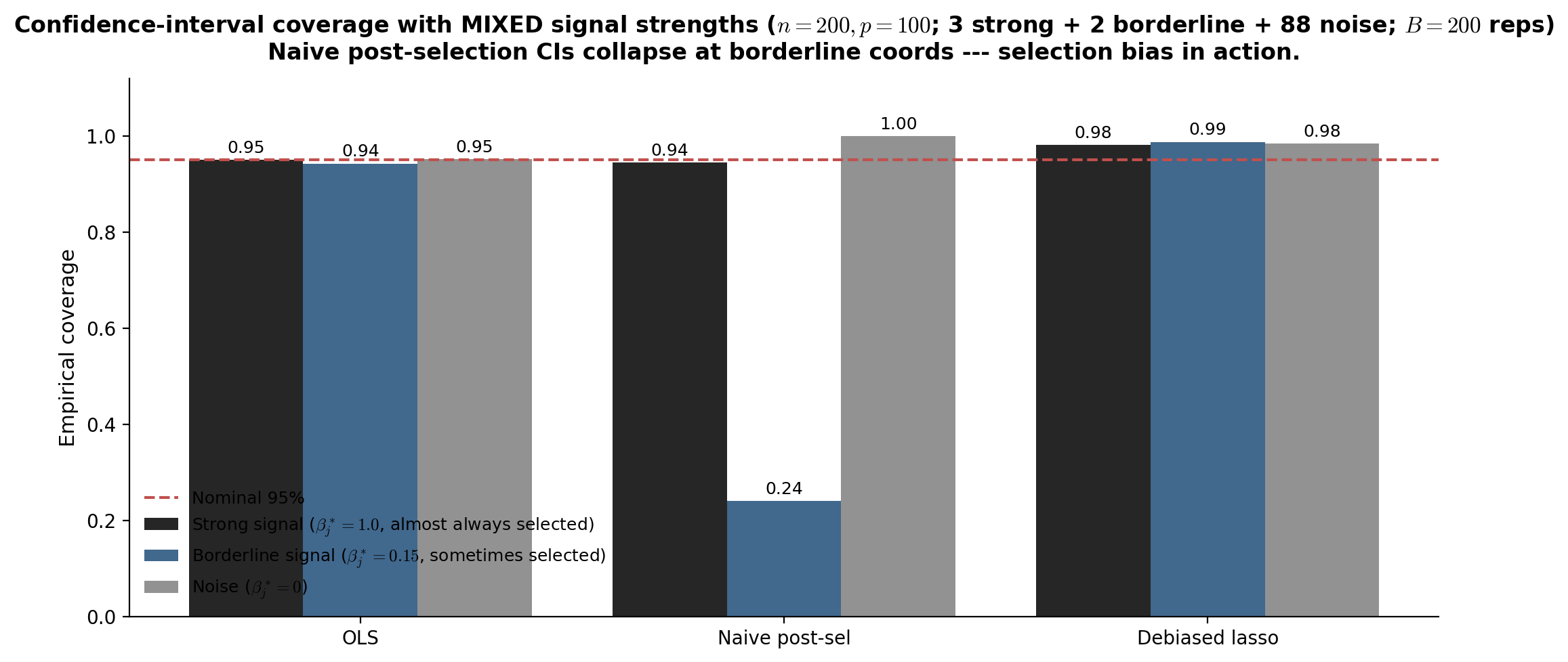
Method	Strong (β* = 1.0)	Borderline (β* = 0.15)	Noise (β* = 0)
OLS (gold standard)	95.0%	94.3%	95.1%
Naive post-selection	94.5%	24.0%	100.0%
Debiased lasso	98.2%	98.8%	98.4%

The headline is the 24.0% entry: at borderline-strength signals (β* = 0.15), naive post-selection CIs undercover by ~70 percentage points. Strong signals (β* = 1.0) are always selected and stably estimated, so the naive procedure happens to cover near nominal; noise coords are typically unselected, making the naive CI degenerate at {0} which trivially covers β* = 0. The OLS baseline (available here because p < n) and the debiased lasso both recover ~95% coverage uniformly across coord types. At p > n where OLS is infeasible, the debiased lasso with nodewise-M̂ is the only valid CI procedure of the three.

§11. Generalized lasso for non-Gaussian responses

Everything in §§1–10 was developed for the Gaussian linear model: $\mathbf{y} = \mathbf{X} \boldsymbol\beta^* + \boldsymbol\varepsilon$ with $\boldsymbol\varepsilon$ iid $\mathcal{N}(\mathbf{0}, \sigma^2 \mathbf{I})$, squared-error loss, soft-thresholding KKT solution. The lasso framework extends naturally to generalized linear models (GLMs) — replacing the squared-error loss with the negative log-likelihood of any GLM family — and most of the topic’s results carry over. This section covers two specific extensions (logistic, Poisson), the general IRLS-with-soft-thresholding solver, and the GLM-debiased-lasso construction for inference.

The math is mostly mechanical: substitute the GLM log-likelihood for the Gaussian one, re-derive the KKT conditions with the new gradient/Hessian, run a similar oracle-inequality argument with sub-Gaussian-replaced-by-sub-exponential noise tail bounds. The conclusions are qualitatively the same — sparsity-adaptive prediction risk under RE, sign-consistency under IC, debiased-lasso CIs at the same $\sqrt n$ rate. We sketch the changes without re-deriving the proofs.

The implementation story is similarly straightforward: scikit-learn’s LogisticRegression(penalty='l1') for binary responses, PoissonRegressor (in sklearn.linear_model) and glmnet for count responses; the underlying solvers are coordinate-descent-with-IRLS or proximal-gradient variants of the Gaussian solvers from §3.

§11.1 Logistic lasso for binary classification

For binary response $y_i \in \{0, 1\}$ with $\mathbb{P}(y_i = 1 \mid \mathbf{x}_i) = \sigma(\mathbf{x}_i^\top \boldsymbol\beta)$ where $\sigma(z) = 1/(1 + e^{-z})$ is the logistic function, the negative log-likelihood per observation is

$$\ell(y_i, \mathbf{x}_i^\top \boldsymbol\beta) = -y_i \, \mathbf{x}_i^\top \boldsymbol\beta + \log(1 + \exp(\mathbf{x}_i^\top \boldsymbol\beta)).$$

The logistic lasso is the L1-penalized negative log-likelihood:

$$\hat{\boldsymbol\beta}^{\text{logistic-lasso}}(\lambda) = \arg\min_{\boldsymbol\beta \in \mathbb{R}^p} \frac{1}{n} \sum_{i=1}^n \ell(y_i, \mathbf{x}_i^\top \boldsymbol\beta) + \lambda \|\boldsymbol\beta\|_1.$$

The objective is convex (the negative log-likelihood is convex; sum of convex; L1 is convex). Two structural differences from the Gaussian case:

No closed-form even on orthogonal designs. The logistic loss is non-quadratic, so the orthogonal-design trick from §3.1 — which reduced the Gaussian lasso to $p$ univariate problems with closed-form solutions — fails. Each coordinate update involves a non-trivial root-finding problem.

The Hessian is data-dependent. For the Gaussian case, $\nabla^2 \ell = \mathbf{X}^\top \mathbf{X} / n$ — independent of $\boldsymbol\beta$ and of $\mathbf{y}$. For logistic, $\nabla^2 \ell = \mathbf{X}^\top \mathbf{W}(\boldsymbol\beta) \mathbf{X} / n$ where $\mathbf{W}(\boldsymbol\beta) = \text{diag}(\sigma(\mathbf{x}_i^\top \boldsymbol\beta)(1 - \sigma(\mathbf{x}_i^\top \boldsymbol\beta)))$ — a $\boldsymbol\beta$-dependent diagonal weighting. This makes the conditioning of the Hessian state-dependent: when many predicted probabilities are near 0 or 1 (extreme classes), $\mathbf{W}$ has small entries and the Hessian is poorly conditioned.

Solver: cyclic coordinate descent with IRLS quadratic approximations. At each outer iteration, form a quadratic approximation of the logistic loss around the current $\boldsymbol\beta^{(t)}$:

$$\ell(\mathbf{y}, \mathbf{X} \boldsymbol\beta) \approx \ell(\mathbf{y}, \mathbf{X} \boldsymbol\beta^{(t)}) + \nabla \ell^\top (\boldsymbol\beta - \boldsymbol\beta^{(t)}) + \frac{1}{2} (\boldsymbol\beta - \boldsymbol\beta^{(t)})^\top \nabla^2 \ell \, (\boldsymbol\beta - \boldsymbol\beta^{(t)}),$$

which is a weighted Gaussian lasso in $\boldsymbol\beta$. Apply Gaussian-lasso coordinate descent (§3.2) to this subproblem; the solution becomes $\boldsymbol\beta^{(t+1)}$. Iterate until convergence. This is the iteratively reweighted least squares (IRLS) framework, the same iteration used for unpenalized GLM fitting (cf. McCullagh-Nelder 1989) with a soft-thresholding modification at each coordinate update.

scikit-learn’s LogisticRegression(penalty='l1', solver='saga') uses a stochastic-average-gradient variant of this scheme; solver='liblinear' uses the dual coordinate descent of Yuan-Ho-Lin (2012), faster on small problems. glmnet’s logistic variant uses outer-IRLS-plus-inner-Gaussian-coordinate-descent and is the practical reference implementation.

Theory carries over. The §5 oracle inequality has a logistic analog: under restricted-eigenvalue (with the design matrix replaced by $\mathbf{W}^{1/2}(\boldsymbol\beta) \mathbf{X}$ to account for the GLM weighting) and the lasso initial $\hat{\boldsymbol\beta}^{\text{logistic-lasso}}$, the prediction risk in deviance terms is bounded by $C \sigma^2 s \log(p) / n$ for an appropriately defined $\sigma$ that depends on the GLM family (van de Geer 2008, Bühlmann-van de Geer 2011 §6). The constants are messier than the Gaussian case but the rate is identical.

§11.2 Poisson lasso for count data

For count response $y_i \in \{0, 1, 2, \dots\}$ with $y_i \mid \mathbf{x}_i \sim \mathrm{Poisson}(\exp(\mathbf{x}_i^\top \boldsymbol\beta))$, the negative log-likelihood is

$$\ell(y_i, \mathbf{x}_i^\top \boldsymbol\beta) = -y_i \, \mathbf{x}_i^\top \boldsymbol\beta + \exp(\mathbf{x}_i^\top \boldsymbol\beta) + \log(y_i!),$$

with the constant $\log(y_i!)$ irrelevant for optimization. The Poisson lasso has the same form as the logistic case:

$$\hat{\boldsymbol\beta}^{\text{Poisson-lasso}}(\lambda) = \arg\min_{\boldsymbol\beta \in \mathbb{R}^p} \frac{1}{n} \sum_{i=1}^n \ell(y_i, \mathbf{x}_i^\top \boldsymbol\beta) + \lambda \|\boldsymbol\beta\|_1.$$

Convex objective, same IRLS-with-coordinate-descent solver pattern, no closed form. The Hessian weighting is $\mathbf{W}(\boldsymbol\beta) = \text{diag}(\exp(\mathbf{x}_i^\top \boldsymbol\beta))$ — the predicted Poisson means.

Useful applications. Genome-wide association studies with rare-variant counts, web traffic prediction, text n-gram occurrence counts, insurance claim counts. The Poisson lasso is the natural sparse-regression tool for any rate-modeling problem.

Caveat: overdispersion. Real count data often has variance exceeding the Poisson assumption ($\mathbb{V}\mathrm{ar}(y_i) > \mathbb{E}[y_i]$). The negative-binomial lasso handles this by adding an overdispersion parameter; statsmodels.NegativeBinomial(penalty='elastic_net') is the standard implementation.

scikit-learn provides PoissonRegressor for unpenalized Poisson regression; for the penalized version, glmnet (via glmnetpy Python bindings) is the reference. A pure-NumPy implementation is straightforward via the IRLS framework but rarely needed in practice.

§11.3 Inference extensions for GLMs

The §10 debiased-lasso construction generalizes from squared-error loss to any GLM negative log-likelihood. The key change: the matrix $\hat{\mathbf{M}}$ now approximates the inverse of the GLM Hessian $\nabla^2 \ell(\hat{\boldsymbol\beta}) = \mathbf{X}^\top \mathbf{W}(\hat{\boldsymbol\beta}) \mathbf{X} / n$, not the unweighted Gram $\mathbf{X}^\top \mathbf{X} / n$.

The GLM-debiased lasso. Given a lasso initial $\hat{\boldsymbol\beta}^{\text{GLM-lasso}}$ and a matrix $\hat{\mathbf{M}}$ approximating the inverse GLM Hessian:

$$\hat{\boldsymbol\beta}^{\text{GLM-db}} := \hat{\boldsymbol\beta}^{\text{GLM-lasso}} + \frac{1}{n} \hat{\mathbf{M}} \mathbf{X}^\top \big(\mathbf{y} - g^{-1}(\mathbf{X} \hat{\boldsymbol\beta}^{\text{GLM-lasso}})\big),$$

where $g^{-1}$ is the GLM inverse-link function ($\sigma$ for logistic, $\exp$ for Poisson). The construction has the same one-step Newton interpretation as the Gaussian case: starting from the biased lasso, take one Newton step toward the unbiased solution.

Nodewise lasso for $\hat{\mathbf{M}}$ in GLMs. The GLM-Hessian-inverse $\hat{\mathbf{M}}$ is constructed by a weighted nodewise lasso: regress each feature $\mathbf{X}_j$ on $\mathbf{X}_{-j}$ with sample weights $w_i = (\mathbf{W}(\hat{\boldsymbol\beta}))_{ii}$ — the same weights that appear in the GLM Hessian. The resulting $\hat{\mathbf{M}}$ approximates $(\mathbf{X}^\top \mathbf{W}(\hat{\boldsymbol\beta}) \mathbf{X} / n)^{-1}$ in the same row-by-row sense as in §10.3.

Asymptotic normality (van de Geer-Bühlmann-Ritov-Dezeure 2014, Theorem 3.1). Under analogous conditions to Theorem 1 of §10.4 — sub-Gaussian design, sparse population GLM-Hessian inverse, $s$-sparse $\boldsymbol\beta^*$, sample-size scaling $n \gg \max(s, s_M) (\log p)^2$ — the GLM-debiased lasso satisfies

$$\sqrt n (\hat\beta_j^{\text{GLM-db}} - \beta^*_j) \overset{d}{\to} \mathcal{N}\big(0, \, \mathrm{var}_j\big),$$

with $\mathrm{var}_j$ given explicitly in terms of the GLM Hessian and the noise structure. Confidence intervals and hypothesis tests follow the same recipe as §10.4.

Practical note. The GLM-debiased lasso is implemented in the hdi R package (Dezeure-Bühlmann-Meier-Meinshausen 2015) for logistic and Poisson families. Python implementations are less mature; desparsified-lasso covers the Gaussian case but not the GLM extension as of this writing. For applications, fitting the GLM lasso via LogisticRegression(penalty='l1') and computing CIs via R’s hdi package is the standard pipeline.

The bigger picture: lasso as a unified penalized-likelihood framework. The lasso’s L1 penalty is a regularizer, not a likelihood-specific construction. It composes with any convex log-likelihood — Gaussian (squared error), Bernoulli (logistic), Poisson (count), Cox (survival), multinomial (multiclass) — to give a family of sparse penalized estimators. Each instance has the same structural flavor (sparsity, bias, IC for selection, RE for prediction, debiased inference) with family-specific computational and statistical details. Friedman-Hastie-Tibshirani (2010, “Regularization Paths for Generalized Linear Models via Coordinate Descent”) is the canonical computational reference; Bühlmann-van de Geer (2011, Statistics for High-Dimensional Data) is the canonical statistical reference covering all families uniformly.

The forward pointer from §11 to the rest of formalML: the GLM-lasso framework is the foundation for causal-inference-methods (T6, planned) — propensity-score and outcome-regression nuisance models with binary or count outcomes use the logistic and Poisson lassos as the natural sparse estimators. The §10 debiased-lasso machinery extends to those nuisance models, giving valid CIs for treatment effects under the double/debiased ML framework (Chernozhukov et al. 2018, covered in §12.1 below).

§12. Connections, applications, and limits

This is the closing section. The lasso is one of the most widely-used algorithms in modern statistics — it shows up as a standalone estimator, as a nuisance estimator inside larger inferential pipelines, and as the conceptual ancestor of an entire family of penalized methods (group lasso, fused lasso, generalized lasso, structured-sparsity penalties). The §§5–10 results we’ve developed for the standard L1-penalized lasso transfer with appropriate modifications to most of these descendants.

This section traces five sets of connections. §12.1 covers the lasso’s role inside double/debiased ML — the dominant modern framework for inference on causal and structural parameters with high-dim nuisance. §12.2 zooms in on causal inference with high-dim confounders, the most consequential application of DML in practice. §12.3 points at the Bayesian counterpart, where horseshoe and spike-and-slab priors achieve approximate sparsity through a different mechanism. §12.4 catalogs where the lasso breaks down in practice — the regimes where the §5–10 theory either fails or requires substantial adaptation. §12.5 lists the forward pointers in formalML — the topics that build on this one.

§12.1 Double / debiased ML (Chernozhukov et al. 2018)

The §10 debiased lasso targets inference on individual coefficients of a high-dim linear regression. Double / debiased machine learning (DML; Chernozhukov-Chetverikov-Demirer-Duflo-Hansen-Newey-Robins 2018) generalizes this to inference on a low-dim target parameter $\theta$ in a model where the nuisance is high-dimensional and estimable by any sufficiently regular ML method — the lasso, random forests, neural networks, gradient boosting. The framework is the modern foundation for treatment-effect inference in observational studies, instrumental-variable regression with many instruments, structural-econometrics estimation, and any other setting where a target parameter is identified by a moment condition involving a high-dim nuisance.

The setup. Suppose the target $\theta_0 \in \mathbb{R}$ is identified by a moment condition

$$\mathbb{E}[\psi(W; \theta_0, \eta_0)] = 0,$$

where $W$ is the observed data, $\psi$ is a known score function, and $\eta_0$ is a high-dimensional nuisance function. The naive plug-in estimator $\hat\theta$ solves $\frac{1}{n} \sum_i \psi(W_i; \hat\theta, \hat\eta) = 0$ where $\hat\eta$ is some ML estimate of $\eta_0$. This is biased: the regularization in $\hat\eta$ propagates into $\hat\theta$, and the resulting estimate has bias of order $1/n^a$ for some $a < 1/2$ — slower than $\sqrt n$ — so confidence intervals based on the naive plug-in undercover.

The two ingredients. DML fixes the naive plug-in via two ingredients used together:

1. Neyman orthogonality. The score $\psi$ must satisfy $\partial_\eta \mathbb{E}[\psi(W; \theta_0, \eta_0)] = 0$ at the true $(\theta_0, \eta_0)$ — the moment condition is insensitive to first-order errors in the nuisance. Constructing such an orthogonal score from an arbitrary moment condition is a calculation: typically subtract off the projection onto the nuisance-tangent space (the influence-function correction).

2. Cross-fitting. Split the data into $K$ folds. For each $i$ in fold $k$, use a nuisance estimate $\hat\eta^{(-k)}$ trained on the data minus fold $k$. This decouples $\hat\eta$ from the residual structure used in the moment condition, eliminating an $O(\sqrt n)$ overfitting bias that the naive in-sample plug-in would have. Cross-fitting is essentially K-fold CV applied to estimation rather than to model selection.

The lasso’s role. The DML framework is silent on which ML method estimates $\hat\eta$ — any method achieving the $o_p(n^{-1/4})$ rate works. The lasso is the standard choice when $\eta_0$ is a sparse high-dim regression, both because it has the right rate (the §5 oracle inequality gives $\|\hat{\boldsymbol\beta}^{\text{lasso}} - \boldsymbol\beta^*\|_2 = O_p(\sqrt{s\log(p)/n})$, beating $n^{-1/4}$ when $s \log p / n \to 0$) and because it’s computationally cheap. Random forests, boosting, and neural networks are alternatives at different parts of the bias-variance spectrum.

Connection to debiased lasso (§10). The §10 debiased lasso is, in a sense, “DML for the special case of inference on an individual regression coefficient.” The one-step Newton correction can be re-derived as the application of the DML influence-function machinery to the moment condition $\mathbb{E}[X_j(Y - X^\top \beta_0)] = 0$. Both rely on Neyman-orthogonal scores; both achieve $\sqrt n$ asymptotic normality despite a regularized nuisance estimator.

§12.2 High-dim confounder adjustment in causal inference

The most consequential DML application is causal inference with many confounders. Setup: observational data $\{(D_i, X_i, Y_i)\}_{i=1}^n$ where $D_i \in \{0, 1\}$ is a binary treatment, $X_i \in \mathbb{R}^p$ is a vector of confounders, and $Y_i \in \mathbb{R}$ is the outcome. Goal: estimate the average treatment effect $\tau = \mathbb{E}[Y_i(1) - Y_i(0)]$, where $Y_i(d)$ is the potential outcome under treatment $d$ (unobserved counterfactual under the unrealized treatment).

Identification under standard assumptions (unconfoundedness $Y(d) \perp D \mid X$, overlap $0 < \mathbb{P}(D = 1 \mid X) < 1$) gives

$$\tau = \mathbb{E}\left[\mu(X, 1) - \mu(X, 0) + \frac{D - \pi(X)}{\pi(X)(1 - \pi(X))} (Y - \mu(X, D))\right],$$

the augmented inverse-propensity-weighting (AIPW) representation, where $\pi(x) := \mathbb{P}(D = 1 \mid X = x)$ is the propensity score and $\mu(x, d) := \mathbb{E}[Y \mid X = x, D = d]$ is the outcome regression. Both nuisance functions are high-dim regression problems; both can be estimated by lasso (logistic for $\pi$, Gaussian for $\mu$).

The AIPW representation is doubly robust (Robins-Rotnitzky-Zhao 1994): the moment condition is satisfied if either $\hat\pi$ or $\hat\mu$ is consistent (not necessarily both). DML strengthens this: under $o_p(n^{-1/4})$ rates for both $\hat\pi$ and $\hat\mu$ (achievable by lasso under sparsity), the cross-fit DML estimator $\hat\tau^{\mathrm{DML}}$ is $\sqrt n$-consistent and asymptotically normal with the semiparametrically efficient variance, regardless of how slow the nuisance rates are.

The practical pipeline. (i) Fit $\hat\pi$ via LogisticRegression(penalty='l1') in cross-fitted form. (ii) Fit $\hat\mu(\cdot, 0)$ and $\hat\mu(\cdot, 1)$ via Lasso in cross-fitted form (separate models for treated and control). (iii) Plug into the AIPW formula. (iv) Compute the standard error from the empirical influence function. (v) Form CI / hypothesis test.

This pipeline is implemented in Python in econml (Microsoft Research) and doubleml (Bach et al.), and in R in the DoubleML package. It’s the standard observational-causal-inference workflow for moderate-to-high-dim confounder vectors. Forward pointer: T6 causal-inference-methods (coming soon) will cover this in detail, including extensions to dynamic treatments, instrumental variables, and partial identification.

§12.3 Sparse-Bayesian alternatives

The lasso’s L1 penalty has a Bayesian interpretation: it’s the negative log-prior of an iid Laplace prior $\beta_j \sim \mathrm{Laplace}(0, 1/\lambda)$, so the lasso estimator is the posterior mode (MAP) under that prior. The posterior mean under the same prior is dense — Bayesian inference based on the Laplace prior doesn’t produce sparse point estimates, only sparse modes.

The Bayesian counterpart of the lasso is a class of priors that produce approximate sparsity in the posterior — most posterior mass concentrated near zero, with heavy tails for the active coefficients. Two main families, both detailed in Sparse Bayesian Priors:

• Horseshoe (Carvalho-Polson-Scott 2010). $\beta_j \sim \mathcal{N}(0, \lambda_j^2 \tau^2)$ with $\lambda_j \sim C^+(0, 1)$ (half-Cauchy local scales) and $\tau \sim C^+(0, 1)$ (global scale). The half-Cauchy local scales have a pole at zero (heavy shrinkage of small signals) and polynomial tails (vanishing shrinkage of large signals) — qualitatively the inverse of the lasso’s constant-shrinkage behavior, so the active-coefficient bias from §4.1 is avoided.
• Spike-and-slab (Mitchell-Beauchamp 1988; George-McCulloch 1993). $\beta_j \sim (1 - w) \cdot \delta_0 + w \cdot \mathcal{N}(0, \sigma^2)$ — a discrete mixture of a point mass at zero (spike) and a wide Gaussian (slab). Posterior puts probability $\hat w_j$ on $\beta_j \neq 0$, giving a natural variable-selection probability.

Trade-offs. Bayesian methods give native uncertainty quantification — credible intervals come for free from the posterior, no debiased-lasso construction needed. The cost: posterior sampling (HMC, NUTS) is computationally expensive at scale, typically 100×–1000× slower than the lasso for the same problem. The lasso wins on speed and the Bayesian methods win on inferential clarity; the practical choice depends on whether $n, p$ scales make MCMC tractable. Forward pointer: Sparse Bayesian Priors covers the full Bayesian sparsity framework — horseshoe, spike-and-slab, R2-D2, regularized horseshoe, and their computational implementations in PyMC and NumPyro.

§12.4 Where the lasso breaks down

The lasso has known failure modes beyond the §6.2 / §9.4 IC and RE failures. Five worth flagging:

Highly correlated features. Already covered (§6.1, §9.4). Recap: lasso flips arbitrarily between correlated features in the active set; elastic net is the standard remedy.

Ultra-high-dimensional regimes ($p > 10^6$). Coordinate descent’s per-iteration cost is $O(np)$ — proportional to the data size. At $p > 10^6$ with $n$ in the thousands, even one coordinate-descent pass takes seconds; full convergence with CV-tuned $\lambda$ becomes computationally prohibitive. Sure independence screening (Fan-Lv 2008): a preprocessing step that filters $p$ down to $O(n)$ candidates by ranking $|\mathbf{X}_j^\top \mathbf{y}|$, then runs the lasso on the reduced feature set. Loses some precision but keeps the workflow tractable. For genuine $p \gg n^{10}$ regimes (some genomics applications), the screening-then-lasso pipeline is standard.

Heavy-tailed (non-sub-Gaussian) noise. The §5.5 deviation step required $\boldsymbol\varepsilon$ to be sub-Gaussian. With heavier tails (say, $\boldsymbol\varepsilon$ Cauchy or Student-$t$ with low degrees of freedom), the maximal inequality $\|\mathbf{X}^\top \boldsymbol\varepsilon / n\|_\infty \le \lambda/2$ fails to hold with the lasso’s standard $\lambda \asymp \sigma\sqrt{\log p / n}$ — the noise has too-large rare excursions. Quantile / median regression lasso (Belloni-Chernozhukov 2011): replace the squared-error loss with the check function $\rho_\tau(u) = u(\tau - \mathbb{1}\{u < 0\})$, giving an L1-penalized quantile regression. Robust to heavy tails because the check loss penalizes residuals linearly, not quadratically. The estimator achieves the same $\sqrt{s \log p / n}$ rate under weaker noise assumptions but requires a different solver (linear programming or smoothed coordinate descent).

Time-series and spatially correlated observations. The lasso assumes iid observations. With correlated observations (autoregressive errors in time series, spatial random fields), the standard $\lambda$-tuning criteria (CV, BIC) become biased — they underestimate the prediction error because nearby training and test points share information. Block-CV (block-wise leave-one-out where each block is a contiguous time window or spatial region) is the standard remedy. Theoretical guarantees under dependence are looser; the most general result is Wong-Li-Tewari (2020) for stationary time series.

Causal lasso interpretation pitfalls. A frequent misuse: interpreting the lasso’s selected coefficients as “causal effects.” The lasso minimizes prediction error on the observed data; the resulting coefficients are predictively useful but not necessarily causally interpretable unless the design satisfies specific structural assumptions (e.g., randomized treatment, valid instruments). The §12.1–§12.2 DML / AIPW pipeline is the right framework when causal interpretation is the goal — the lasso’s role is as a nuisance estimator, not as the producer of causal coefficients.

§12.5 Forward pointers in formalML

The lasso machinery from this topic feeds into several planned formalML topics:

• Semiparametric Inference (coming soon). The DML framework introduced in §12.1 generalizes substantially: any target parameter $\theta_0$ identified by a moment condition with high-dim nuisance can be estimated $\sqrt n$-consistently using cross-fitted ML estimates of the nuisance. The lasso is one of several admissible nuisance estimators (alongside random forests, gradient boosting, neural networks). The semiparametric-inference topic will treat the unified framework — Neyman orthogonal scores, the $o_p(n^{-1/4})$ nuisance rate condition, the practical pipeline — at the level needed for applied econometrics and causal inference.

• Causal Inference Methods (coming soon). Treatment-effect inference with high-dim confounders (§12.2) is the headline application of the DML framework. The causal-inference-methods topic will cover the full observational-causal-inference workflow: identification assumptions (unconfoundedness, overlap), the AIPW representation, double-robust efficient scores, the DML estimator and its CI / hypothesis tests, sensitivity analysis to unmeasured confounding, dynamic treatment regimes, and the connection to instrumental variables. Throughout, the lasso (logistic for propensity, Gaussian for outcome) is the default nuisance estimator.

• PAC-Bayes Bounds (coming soon). Catoni’s (2007) PAC-Bayesian framework gives an alternative theoretical perspective on sparse regression: instead of the §5 oracle inequality (frequentist, RE-based), use a PAC-Bayes bound with a sparsity-favoring prior to derive a closely-related risk bound. The PAC-Bayes prior is structurally similar to the Bayesian sparsity priors of §12.3; the resulting estimator is closer to the posterior mean than to the lasso. The pac-bayes-bounds topic will treat this connection.

• Bayesian Neural Networks. Sparse priors on neural network weights — particularly horseshoe priors on the input-layer weights — give automatic feature selection in deep models. The §12.3 Bayesian sparsity framework, scaled up to neural-net parameter counts, is the foundation for this. The bayesian-neural-networks topic covers practical implementations (HMC, variational inference) and the recovery guarantees.

• Density Ratio Estimation (coming soon). Estimating $r(x) = p_2(x) / p_1(x)$ from samples of $p_1$ and $p_2$ is a related problem to regression — KLIEP (Kullback-Leibler importance estimation procedure) and its sparse-regularized variants reduce to convex optimization problems that look very much like the lasso. The connection isn’t immediate, but the algorithmic and theoretical machinery transfers.

The closing thesis. The lasso is one of the most successful algorithms in modern statistics because it occupies a sweet spot in the bias-variance-computability triangle. Sparsity bias is small under reasonable conditions; sparsity-adapted variance is the lowest of any L1-style estimator; the convex-optimization formulation makes computation tractable at scales where every pre-2000 alternative was infeasible. The §5 oracle inequality and the §10 debiased-lasso construction together make the lasso the standard tool for both prediction and inference in the sparse high-dim regime, with adaptations (elastic net, adaptive lasso, GLM-lasso, DML-lasso) covering the cases where the basic version doesn’t fit. We’ve worked through the full pipeline; the rest of the formalML topic graph picks up the threads from here.