Double Descent

Motivation: the empirical phenomenon

The textbook bias-variance U-curve as the picture being revised

Anyone who has taken a first course in machine learning carries around a picture of generalization. Test error decomposes into bias, variance, and irreducible noise; as model complexity grows, bias falls and variance rises; and somewhere in between is the sweet spot we call the optimal model. The picture is universally drawn as a U-curve, and it underwrites every regularization heuristic from ridge to early stopping to dropout. If we want to generalize, we don’t make our model bigger — we make it the right size.

This picture comes from the classical learning-theory regime where the number of parameters $p$ is small relative to the number of training points $n$. The U-curve has decades of empirical and theoretical support in that regime. VC bounds, structural risk minimization, AIC, BIC, and cross-validation all give different recipes for finding the bottom of the U, and in the underparameterized regime they roughly agree. The picture is right.

What the picture leaves out is what happens past the bottom. If $p$ is small the right edge of the U is just “variance keeps growing as the model overfits more.” The picture says nothing specific about $p > n$, because nobody used to fit models in that regime. When statisticians said “more parameters than data points,” they meant “the problem is ill-posed and the answer is to either get more data or shrink the model class.” That answer was correct as long as we were planning to use OLS — and as long as we didn’t have a way to pick one of the infinitely many interpolators that exist past the threshold.

The reason this matters now is that modern neural networks live in the $p \gg n$ regime by orders of magnitude. ResNet-50 has 25M parameters; ImageNet has 1.3M images. GPT-3 has 175B parameters; the training corpus has somewhere between $10^{10}$ and $10^{12}$ tokens. In every case the model class is wildly larger than what classical learning theory says we can hope to generalize from. The networks generalize anyway. Why is the question this topic is built around — and the first step is to recognize that the U-curve isn’t wrong, but it tells the story of only the first half of the picture.

The empirical phenomenon: a synthetic linear-regression demo

Let’s make this empirical before we make it formal. The cleanest experimental setup is the one Hastie, Montanari, Rosset, and Tibshirani (2022) analyze: linear regression with isotropic Gaussian features.

We fix an ambient feature dimension $P = 200$, a training-set size $n = 50$, a noise level $\sigma^2 = 1$, and a signal-to-noise ratio $\mathrm{SNR} = \|\beta^*\|^2 / \sigma^2 = 1$. We draw a fixed true coefficient vector $\beta^* \in \mathbb{R}^P$ uniformly on the sphere of radius $\sigma \sqrt{\mathrm{SNR}}$, and for each replicate $b \in \{1, \ldots, B\}$ we generate

$$X^{(b)} \in \mathbb{R}^{n \times P}, \quad X^{(b)}_{ij} \stackrel{\text{i.i.d.}}{\sim} \mathcal{N}(0, 1), \qquad y^{(b)} = X^{(b)} \beta^* + \varepsilon^{(b)}, \quad \varepsilon^{(b)} \sim \mathcal{N}(0, \sigma^2 I_n).$$

For each model size $p \in \{1, 2, \ldots, P\}$, we use only the first $p$ columns of $X^{(b)}$ to fit a linear model. When $p \leq n$ this is ordinary least squares; when $p > n$ the system is underdetermined and we pick the minimum-norm interpolator via the SVD pseudoinverse:

$$\hat\beta^{\dagger}_p \;=\; \big(X^{(b)}_{:,\,1:p}\big)^{+} \, y^{(b)} \;=\; V\, \Sigma^{+}\, U^{\top}\, y^{(b)},$$

where $X^{(b)}_{:,\,1:p} = U\Sigma V^{\top}$ is the thin SVD of the truncated design matrix and $\Sigma^{+}$ is the pseudoinverse of the singular-value matrix — we invert nonzero singular values and zero out the rest, with a numerical truncation threshold of $\mathrm{rcond} \cdot \sigma_{\max}$.

We evaluate excess test risk against the full signal,

$$\mathrm{ExcessRisk}(p) \;=\; \mathbb{E}\!\left[\big(X^{\top} \hat\beta^{\dagger}_p - X^{\top} \beta^*\big)^{2}\right],$$

where the expectation is over a fresh test point $X \sim \mathcal{N}(0, I_P)$, estimated empirically on a held-out set of 1000 test points and averaged over $B = 50$ replicates. The result is Figure 1.

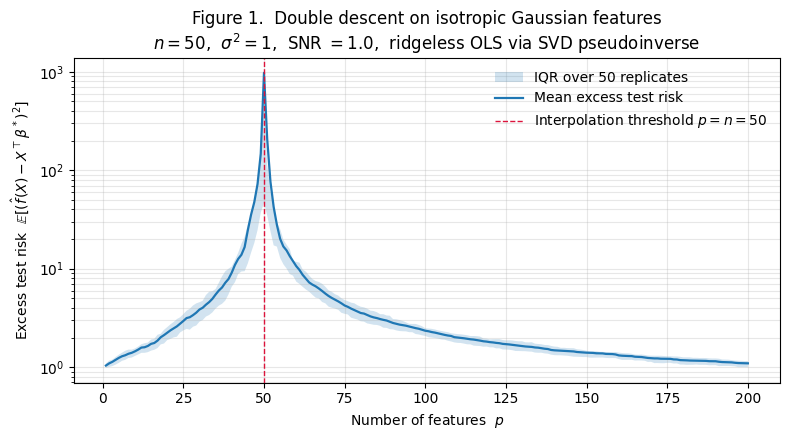
What the curve shows:

• Classical regime $p < n$. Excess risk climbs gently from $\approx 1.04$ at $p = 1$ to $\approx 9.1$ at $p = 40$ and $\approx 147$ at $p = 49$. As we add parameters, bias falls (we capture more of $\beta^*$) but variance rises. For these parameters the variance growth dominates.
• Interpolation threshold $p = n = 50$. The mean excess risk spikes to $\approx 977$ — nearly three orders of magnitude above its neighbors. The IQR band widens dramatically here; the spike is a genuine concentration of the curve, not a single-replicate outlier.
• Overparameterized regime $p > n$. Excess risk crashes back down. By $p = 60$ we’re at $\approx 11$. By $p = 100$ we’re at $\approx 2.3$. At $p = 200 = 4n$, excess risk is $\approx 1.1$ — essentially indistinguishable from the $p = 1$ baseline.

This is double descent. Two descents — one in the classical regime, one past the threshold — separated by a spike at exactly the point where the design matrix becomes square.

A note on the feature choice. The features in Figure 1 are isotropic Gaussian, rather than a structured basis like polynomials or wavelets. This isn’t a cosmetic choice. The clean second descent depends on the random-matrix-theory machinery we develop in §5, which requires the columns of $X$ to behave as approximately i.i.d. random vectors. Polynomial features on a 1D uniform input — the most familiar concrete example — don’t satisfy this, and the second descent fails to appear cleanly. The right way to think about the isotropic-Gaussian features here is as a stand-in for the random representations a neural network learns in the wide regime; §8 returns to this with the random-features model and makes the connection precise.

Nakkiran 2020: the deep-net version of the same curve

The phenomenon we just saw isn’t a quirk of linear regression. Nakkiran et al. (2020) showed that the same shape appears in modern neural networks across multiple axes:

• Width-wise. At fixed depth and training-set size, test error spikes at a critical width and falls again past it. For ResNet-18 on CIFAR-10 with 15% label noise, the spike sits at approximately the width where the network has just barely enough capacity to drive training error to zero.
• Depth-wise. At fixed width and training-set size, the same shape appears as a function of depth.
• Epoch-wise. At fixed architecture, test error during training shows a non-monotone descent — improvement, spike near the epoch when training error crosses zero, then improvement again.

What unifies these axes is that the spike always appears at the point where the model just barely manages to interpolate the training set. Before that point we’re in the classical “more capacity hurts” regime. After that point we’re in the modern “more capacity helps” regime. Section 10 returns to this with a sidebar reproducing the width-wise curve on a small MLP toy; the rest of the topic establishes why the linear theory we develop predicts this exact shape.

What’s special about the interpolation threshold $p = n$

The spike in Figure 1 isn’t an artifact of the random initialization or the small sample size. It’s a generic consequence of what happens to a linear system when the number of features matches the number of training points.

Let’s name three regimes by what the design matrix $X \in \mathbb{R}^{n \times p}$ looks like.

• Underparameterized regime $p < n$. The matrix is tall. The normal equations $X^{\top} X \hat\beta = X^{\top} y$ have a unique solution that minimizes the squared training error. There’s no requirement that this solution interpolate the training points; generically, it can’t.
• Overparameterized regime $p > n$. The matrix is wide. The normal equations are underdetermined: any $\beta$ with $X\beta = y$ achieves zero training error, and there’s an entire $(p - n)$-dimensional affine subspace of such solutions. We need an additional principle to pick one. The SVD pseudoinverse picks the element of that subspace with smallest $\ell_2$-norm — what we’ll call the minimum-norm interpolator $\hat\beta^{\dagger}$ in §4.
• Interpolation threshold $p = n$. The matrix is square. Under generic conditions on $X$ — Gaussian features, random subsets of an orthogonal basis, polynomial features at distinct points — the matrix is almost surely invertible, and the unique solution $\hat\beta = X^{-1} y$ exactly interpolates the training data including the noise.

The threshold is special for a reason we can already read off the third bullet: the system has just enough degrees of freedom to interpolate the noise and no slack to absorb it. Algebraically, the condition number $\kappa(X) = \sigma_{\max}(X) / \sigma_{\min}(X)$ diverges as we approach $p = n$ from either side. Geometrically, the smallest singular value of $X$ — which controls how much the noise vector $\varepsilon$ gets amplified into the fitted coefficients — is order $1/\sqrt{n}$ in the well-behaved regime but collapses to order $|n - p| / \sqrt{n}$ near the threshold. The spike in Figure 1 is the manifestation of $1/\sigma_{\min}$ blowing up.

We’ll make all of this precise in §3 with explicit closed-form expressions for the variance, and in §§5–6 with the asymptotic random-matrix-theory machinery that produces the analytic double-descent curve. For now, the moral is: the U-curve breaks at exactly $p = n$ because the linear system has no slack to absorb noise; and the second descent is what happens when we move past the threshold into the regime where there’s room to choose a good interpolator.

Roadmap

The path forward:

• §§2–3 revisit the classical bias-variance / VC / SRM picture and pin down exactly where it breaks. The interpolation threshold is the focus of §3.
• §§4–6 build the analytic double-descent curve from scratch. §4 introduces the minimum-norm interpolator and its SVD expression; §5 introduces the Marchenko–Pastur eigenvalue density that governs the spectrum of $X^{\top}X / n$; §6 gives the closed-form bias-variance decomposition and proves the second descent.
• §§7–8 generalize beyond the basic setup. §7 separates model-wise from sample-wise double descent in the Nakkiran taxonomy. §8 extends to random-features models and connects to the kernel limit.
• §§9–10 explain why explicit regularization isn’t needed for the second descent. §9 proves that gradient descent from zero init converges to the minimum-norm interpolator. §10 is a sidebar on deep double descent.
• §§11–12 discuss effective dimension (why $p \gg n$ can behave like $p < n$ for the right designs) and the modern revision of classical capacity-control theories.
• §§13–14 close with computational notes and an honest accounting of what the linear theory predicts versus what remains open in the deep regime.

The classical story being revised

Bias-variance decomposition and the classical U-curve

The picture from §1.1 has a precise mathematical formulation. Suppose we have a true function $f^*(x) = x^{\top} \beta^*$ and a learned predictor $\hat f(x) = x^{\top} \hat\beta$ trained on a random dataset. The excess test risk at a fixed test point $x$, averaged over the randomness of the training set, is

$$\mathrm{ExcessRisk}(x) \;=\; \mathbb{E}_{\mathrm{train}}\!\left[\big(\hat f(x) - f^*(x)\big)^{2}\right].$$

Adding and subtracting the mean predictor $\bar f(x) := \mathbb{E}_{\mathrm{train}}[\hat f(x)]$ and expanding,

$$\mathrm{ExcessRisk}(x) \;=\; \underbrace{\big(\bar f(x) - f^*(x)\big)^{2}}_{\mathrm{Bias}^{2}(x)} \;+\; \underbrace{\mathbb{E}_{\mathrm{train}}\!\left[\big(\hat f(x) - \bar f(x)\big)^{2}\right]}_{\mathrm{Variance}(x)}.$$

The cross term vanishes — the mean predictor is the $L^2$-projection of $\hat f$ onto constants in training-set space — and we get the canonical decomposition. Squared bias measures how far the average learned predictor sits from the truth; variance measures how much the predictor wobbles around its average across training-set draws.

Averaging over a fresh test point $X$ gives the total excess risk:

$$\mathrm{ExcessRisk} \;=\; \mathbb{E}_{X}\!\left[\mathrm{Bias}^{2}(X)\right] \;+\; \mathbb{E}_{X}\!\left[\mathrm{Variance}(X)\right].$$

The classical bias-variance trade-off is the empirical observation that as we increase model complexity, bias falls but variance rises. To make this concrete, Figure 2 shows the decomposition on a clean textbook setup: polynomial regression on a noisy sine wave, well inside $p \ll n$ so the interpolation-threshold pathology from §1 doesn’t enter.

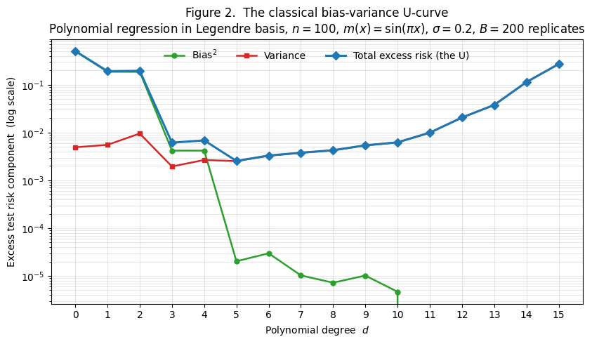
We sample $n = 100$ training points $X_i \sim \mathrm{Uniform}(-1, 1)$ and observe $y_i = \sin(\pi X_i) + \varepsilon_i$ with $\varepsilon_i \sim \mathcal{N}(0, 0.04)$. For each polynomial degree $d \in \{0, 1, \ldots, 15\}$ we fit by ordinary least squares in the Legendre polynomial basis $\{P_0, P_1, \ldots, P_d\}$ — Legendre because the monomial basis is catastrophically ill-conditioned at moderate degrees on $[-1, 1]$, but $P_j(x)$ stays bounded and the design matrix stays well-behaved. We compute bias² and variance by Monte Carlo over $B = 200$ replicates with a shared test set of 1000 points, applying the standard finite-$B$ correction $\mathrm{Bias}^2 \mapsto \mathrm{Bias}^2 - \mathrm{Variance}/B$ to remove the MC bleed-through into the bias estimator.

Three things stand out in Figure 2:

• Bias drops in two steps. From $d = 0$ to $d = 1$ and again from $d = 2$ to $d = 3$ and from $d = 4$ to $d = 5$, with plateaus between. The target $\sin(\pi x)$ is an odd function, so even-degree Legendre polynomials don’t contribute to its approximation; adding an even-degree term doesn’t reduce bias. This staircase pattern is a nice illustration that bias depends on how well the model class can approximate $f^*$, not on the raw parameter count.
• Variance grows roughly linearly with $d$. From $\approx 0.006$ at $d = 0$ to $\approx 0.16$ at $d = 15$. The per-feature variance contribution is approximately $\sigma^{2} / n$ when features are well-conditioned, and we have $d + 1$ features at degree $d$.
• Total has a clear minimum. At $d = 5$, where bias has dropped below the noise floor and variance is still small. By $d = 15$, total excess risk is two orders of magnitude above the minimum — variance has taken over. This is the classical U.

This is the picture the U-curve has stood for since at least Geman, Bienenstock, and Doursat (1992), and it is exactly the right picture for the regime we’re plotting. The textbook recommendation that follows — pick the model complexity that minimizes test error, or use cross-validation to estimate it — is correct in this regime and remains the operating assumption for most of statistics.

VC and SRM: capacity must be controlled

The bias-variance picture in Figure 2 is descriptive, not predictive — we observed the U-curve, but we’d like a theoretical argument for why test error grows with capacity past the bias-variance minimum, and a tool for picking the right capacity before seeing the data.

This is the program of statistical learning theory. The two foundational tools — both shipped formalML topics — are VC dimension (Vapnik and Chervonenkis 1971, formalized in Vapnik 1995) and structural risk minimization (Vapnik 1995). VC dimension gives a combinatorial capacity measure for binary-classification hypothesis classes: the largest sample size on which the class can realize every labeling pattern. Sample-complexity bounds turn this into uniform convergence guarantees of the form

$$\sup_{h \in \mathcal{H}}\, \big|\,\hat L_n(h) - L(h)\,\big| \;=\; O\!\left(\sqrt{\frac{d_{\mathrm{VC}}(\mathcal{H}) \log n + \log(1/\delta)}{n}}\,\right)$$

with probability at least $1 - \delta$ — the generalization gap is controlled by VC capacity relative to sample size.

Structural risk minimization is the algorithmic counterpart: rather than picking a fixed hypothesis class up front, take a nested family $\mathcal{H}_1 \subset \mathcal{H}_2 \subset \cdots$ of increasing capacity and let the data decide where to sit. The SRM estimator picks

$$\hat h_{\mathrm{SRM}} \;\in\; \arg\min_{k}\, \big(\hat L_n(\hat h_k) + \mathrm{pen}(d_k, n, \delta)\big),$$

where $\mathrm{pen}(\cdot)$ is a per-class capacity penalty. The penalty grows with capacity, the training loss falls with capacity, and the SRM estimator picks $\hat k$ where their sum is smallest — exactly the argmin of the bias-variance U-curve, with the penalty playing the role of “predicted variance” and the training loss playing the role of “predicted bias.”

The point for us is that classical learning theory’s central recommendation is to control capacity. Cross-validation, AIC, BIC, ridge, lasso, and early stopping are all operationally capacity-control devices, even when they’re motivated differently. The story is coherent: the U-curve exists, the minimum is somewhere on the underparameterized side, and the regularizer’s job is to find it.

Why $p \gg n$ was historically considered hopeless

Continue the right edge of Figure 2 toward $d = n$. The variance contribution from each additional feature is approximately $\sigma^{2} / (n - d)$ once the design matrix becomes nearly singular — the inverse of the smallest singular value of $X^{\top}X / n$ blows up. By $d = n - 1$ we’re at variance $\sim \sigma^{2}$ per feature, and at $d = n$ the OLS estimator doesn’t exist: $X^{\top}X$ is singular and the normal equations have no unique solution.

Classical statistics’ answer to this was unambiguous: don’t go there. If a problem genuinely has $p \geq n$, the options were three. (i) Get more data. (ii) Pick a smaller model class — feature selection, dimensionality reduction. (iii) Regularize so heavily that the effective capacity drops well below $n$ — ridge with $\lambda \to \infty$, lasso with sparsity constraint $s \ll n$. Hastie, Tibshirani, and Friedman’s Elements of Statistical Learning (2009), the canonical reference for the classical synthesis, devotes its high-dimensional chapter to exactly these three options.

What classical theory did not contemplate, except as a curiosity, was simply solving the underdetermined system $X\beta = y$ for some specific $\beta$ — say the minimum-norm one — and using that as the predictor. The minimum-norm interpolator $\hat\beta^{\dagger} = X^{+} y$ exists for any $p > n$ via the SVD pseudoinverse, and it has zero training error by construction. Classical theory’s reading of “zero training error in the high-dimensional regime” was unambiguous: this is the worst possible overfit. The empirical bias-variance decomposition past the threshold — variance crashing, bias not exploding — wasn’t on the radar because nobody was running the experiment.

What Belkin et al. (2019), Hastie et al. (2022), and Nakkiran et al. (2020) collectively demonstrated is that the minimum-norm interpolator generalizes anyway — sometimes as well as the classical U-curve minimum, often better in the data-poor / overparameterized regimes that modern ML actually inhabits. This is the surprise the topic is built around. The rest of §§3–9 explains why.

Where the classical story holds — and where it doesn’t

The bias-variance decomposition itself is unconditional — it’s just an application of the parallelogram law in $L^{2}$ — and holds for any estimator at any model size, including the minimum-norm interpolator past the threshold. What changes past the threshold is the behavior of the components, not the validity of the decomposition.

Three things break.

• Variance doesn’t keep growing. In the classical regime, variance grows roughly as $\sigma^{2} d / n$ for well-conditioned designs. Past the threshold, the variance of the minimum-norm interpolator scales as $\sigma^{2} n / (p - n)$ for $p > n$ — and decreases with $p$. The intuition is that adding more features past the threshold gives the noise more directions to spread into, each contributing less individually. We make this precise in §6.
• Bias doesn’t drop to zero. With more parameters than data, an unbiased estimator of $\beta^{*}$ doesn’t exist — the minimum-norm interpolator shrinks the projection onto the data subspace and discards the orthogonal complement. The bias of the minimum-norm interpolator approaches $\|\beta^{*}\|^{2} \cdot (1 - n/p)$ as $p \to \infty$. Not zero, but bounded. This is the phenomenon §11 makes precise as “effective dimension.”
• Capacity-control recipes change meaning. Cross-validation still works (it’s a black-box procedure); SRM-style penalties don’t, because classical VC and Rademacher capacity terms become vacuous past the threshold — a class that interpolates every labeling pattern on the training set has trivially $d_{\mathrm{VC}} \geq n$. The flatness and margin theories developed for deep nets are the modern substitutes, which §12 treats.

The classical U-curve is the left half of the picture. The spike at $p = n$ is the transition. The second descent past the threshold is the right half. Sections 3 through 9 build the right half from scratch.

The interpolation threshold

Linear regression setup

Fix notation. We have observations $(X_i, y_i)$ for $i = 1, \ldots, n$ where $X_i \in \mathbb{R}^{p}$ are feature vectors and $y_i \in \mathbb{R}$ are responses. Stack into matrix form: $X \in \mathbb{R}^{n \times p}$ with rows $X_i^{\top}$, and $y \in \mathbb{R}^{n}$.

We assume the linear data-generating model

$$y \;=\; X \beta^{*} + \varepsilon,$$

where $\beta^{*} \in \mathbb{R}^{p}$ is the (unknown) true coefficient vector and $\varepsilon \in \mathbb{R}^{n}$ is noise with $\mathbb{E}[\varepsilon] = 0$ and $\mathrm{Cov}(\varepsilon) = \sigma^{2} I_n$. The OLS estimator is $\hat\beta = \arg\min_{\beta} \|y - X\beta\|^{2}$.

When $X^{\top}X$ is invertible — which requires $p \leq n$ together with $X$ having full column rank — the unique minimizer is $\hat\beta_{\mathrm{OLS}} = (X^{\top}X)^{-1} X^{\top} y$. When $X^{\top}X$ is singular, either because $p > n$ or because columns of $X$ are linearly dependent, the OLS optimization has infinitely many minimizers. For $p > n$ with rows of $X$ in general position, every $\beta$ with $X\beta = y$ achieves zero training error. We need an additional principle to select one. The natural choice, motivated in §§4 and 9, is the minimum-norm interpolator

We use $\hat\beta^{\dagger} = X^{+} y$ as the uniform notation from §4 onward.

The square design at $p = n$: exact interpolation forces noise-fit

At $p = n$ the design matrix is square. For $X$ with independent continuous-distribution entries — Gaussian features being the canonical example — $X$ is almost surely invertible. The system $X \beta = y$ has the unique solution

$$\hat\beta \;=\; X^{-1} y \;=\; X^{-1}(X \beta^{*} + \varepsilon) \;=\; \beta^{*} + X^{-1} \varepsilon.$$

Two things are now visible from this expression.

1. The estimator is unbiased. $\mathbb{E}[\hat\beta] = \beta^{*} + X^{-1} \mathbb{E}[\varepsilon] = \beta^{*}$. No systematic error.
2. The variance is governed entirely by $X^{-1}$. Conditional on $X$, $\mathrm{Cov}(\hat\beta \mid X) = \sigma^{2} (X^{\top}X)^{-1}$.

Expand $X = U\Sigma V^{\top}$ with singular values $s_1 \geq s_2 \geq \cdots \geq s_n > 0$. Then $(X^{\top}X)^{-1} = V\, \mathrm{diag}(s_1^{-2}, \ldots, s_n^{-2})\, V^{\top}$. The expected squared coefficient norm, which equals the trace of this covariance matrix, is

$$\mathbb{E}\big[\|\hat\beta - \beta^{*}\|^{2}\big] \;=\; \sigma^{2}\, \mathrm{tr}\big((X^{\top}X)^{-1}\big) \;=\; \sigma^{2} \sum_{i=1}^{n} s_i^{-2}.$$

This sum is dominated by the smallest singular value $s_n$. If $s_n$ is order $1$, the trace is order $n$ and the noise amplification is modest. If $s_n$ is order $\delta$ for small $\delta$, the trace is order $\delta^{-2}$ and the amplification is huge.

For square iid Gaussian $X$, the smallest singular value has the distribution analyzed by Edelman (1988): $s_n$ scales as $1/\sqrt{n}$ in expectation, with substantial fluctuations. So $\mathbb{E}[\|\hat\beta - \beta^{*}\|^{2}]$ is of order $\sigma^{2} n^{2}$ — enormous noise amplification, growing with sample size rather than shrinking.

The geometric reading: when $X$ is square and just barely invertible, $X^{-1}\varepsilon$ amplifies the noise vector by $1/s_n$ along the direction of $X$‘s least-stable singular vector. Even when $\varepsilon$ has typical Gaussian magnitude, $X^{-1}\varepsilon$ has wild magnitude in that one direction. The fitted $\hat\beta$ inherits the wildness, and the predicted $\hat f(x) = x^{\top}\hat\beta$ inherits it at a random test point.

The unbiasedness is what makes this counterintuitive. We’re not biased, but our variance is so large that $\hat\beta$ is useless. Classical estimation theory has names for this — minimax suboptimality at low signal-to-noise, the curse of unbiasedness in singular models — but the upshot is that we shouldn’t trust unbiasedness as a sufficient property near the threshold.

The condition-number blowup near the threshold

For $p \neq n$, the condition number $\kappa(X^{\top}X) = s_1^{2} / s_{\min(n,p)}^{2}$ measures how singular the design matrix is. We want to know what $\kappa$ looks like as $p$ varies with $n$ fixed.

The Marchenko–Pastur (MP) theorem, which we’ll meet properly in §5, gives the asymptotic answer. For iid features with finite variance, as $n \to \infty$ with $p/n \to \gamma > 0$ fixed, the empirical spectral distribution of $X^{\top}X / n$ converges to the MP density, which is supported on the interval

$$\big[\, (1 - \sqrt\gamma)_{+}^{2},\;\; (1 + \sqrt\gamma)^{2}\,\big],$$

where $(x)_{+} = \max(x, 0)$. Taking square roots and rescaling,

$$\frac{s_{\max}}{\sqrt n} \;\to\; 1 + \sqrt\gamma, \qquad \frac{s_{\min}}{\sqrt n} \;\to\; |1 - \sqrt\gamma|.$$

At $\gamma = 1$ both endpoints contain $0$: $s_{\min}/\sqrt n \to 0$. The condition number $\kappa(X^{\top}X) \to \infty$. This is the analytic origin of the threshold spike. The MP density’s support degenerates to $[0, 4]$ exactly at $\gamma = 1$, and the integral $\int s^{-2}\, \rho_{\mathrm{MP}}(s^{2})\, ds$ diverges.

For finite $n$ the MP prediction is an excellent approximation away from $\gamma = 1$, and Figure 3 (top panel) verifies this directly: the observed $s_{\min}(X / \sqrt n)$ and $s_{\max}(X / \sqrt n)$ overlay the MP predictions $|1 - \sqrt\gamma|$ and $1 + \sqrt\gamma$ across the full sweep. The V-shape at $\gamma = 1$ is unmistakable — and $s_{\min}$ doesn’t quite reach zero at finite $n$ (it’s of order $1/n$), which is what saves the experiment from total numerical failure.

Translating $s_{\min}$ into variance amplification: $\sigma^{2} / s_{\min}^{2}$ scales as $\sigma^{2} / n(1 - \sqrt\gamma)^{2}$ — finite for $\gamma < 1$, blowing up at $\gamma = 1$. §6 turns this scaling into a closed-form analytic curve via integrals against the MP density.

The empirical risk spike: synchronized demonstration

Figure 3 makes the full chain visible. Three panels, all with $p$ on the x-axis and the interpolation threshold $p = n = 50$ marked.

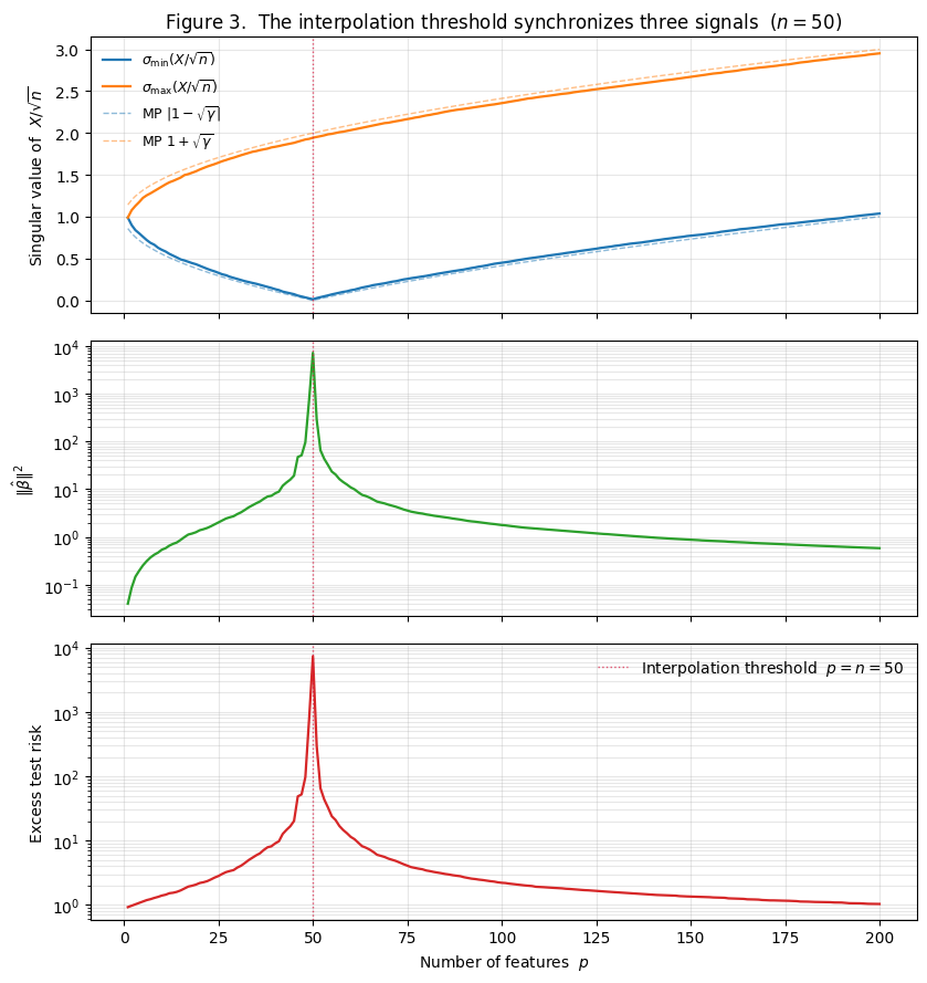
Three panels:

• Top: singular values. $s_{\min}$ V-shapes down to a near-zero minimum at $p = n$, matching the MP prediction $|1 - \sqrt\gamma|$ across the full range. $s_{\max}$ climbs smoothly from $1$ at $p = 1$ to $\approx 3$ at $p = 200$, also matching MP. The agreement is surprisingly good at finite $n = 50$.
• Middle: coefficient norm. $\|\hat\beta\|^{2}$ spikes by five orders of magnitude at $p = n$ — from $\approx 0.04$ at $p = 1$ to $\approx 7000$ at $p = 50$ to $\approx 0.6$ at $p = 200$. The shape exactly mirrors $1 / s_{\min}^{2}$ from the top panel.
• Bottom: excess test risk. Test risk follows $\|\hat\beta\|^{2}$ almost identically: a spike to $\approx 7000$ at $p = n$, recovery to $\approx 1$ at $p = 200$. This is the same data as §1 Figure 1; the new content is its alignment with the eigenvalue and coefficient-norm curves.

The synchronization is the §3 punchline. The interpolation threshold isn’t a special location in any abstract sense — it’s the unique value of $p$ where the design matrix becomes singular, the noise amplification factor blows up, the fitted coefficient norm explodes, and test risk follows. Every spike in the lower two panels of Figure 3 is mechanically caused by the dip in the top panel.

Two consequences worth stating now.

• The spike is intrinsic, not artifactual. Different random initializations, different basis choices, different sample sizes — anything that preserves the structural fact “design matrix becomes square at $p = n$” — will reproduce the spike. The only way to soften it is to explicitly avoid the singularity: ridge regularization adds $\lambda I$ to $X^{\top}X$, which pushes $s_{\min}$ away from zero and smooths the spike. §4 returns to this with the RidgelessVsRidge story.
• The mechanism is purely about $s_{\min}$. Bias barely changes near the threshold (we saw this in §2.4); the spike is all variance, all driven by $1/s_{\min}^{2}$. The post-threshold descent isn’t a separate phenomenon; it’s the eigenvalue distribution reopening past $\gamma = 1$, taking the variance amplification back down with it.

Beyond the threshold: ridgeless regression

The wide regime: infinitely many zero-training-error solutions

When $p > n$, the system $X \beta = y$ has infinitely many solutions. Every $\beta$ satisfying this equation interpolates the training data exactly — zero training error, perfect memorization.

To see why there are infinitely many: with high probability $X \in \mathbb{R}^{n \times p}$ has full row rank, so the linear map $\beta \mapsto X\beta$ is surjective onto $\mathbb{R}^{n}$. The set of solutions to $X\beta = y$ is then a translate of the null space of $X$, $\{\beta : X\beta = y\} = \beta_{0} + \mathrm{null}(X)$, for any particular solution $\beta_{0}$. The null space has dimension $p - n > 0$, so the solution set is a $(p - n)$-dimensional affine subspace. We need a selection principle to pick one element.

The natural choice (Bartlett et al. 2020; Hastie et al. 2022) is the minimum-norm interpolator $\hat\beta^{\dagger} = \arg\min_{\beta : X\beta = y} \|\beta\|^{2}$, for three reasons that come later in the topic.

1. Algorithmic. Gradient descent on $\|X\beta - y\|^{2}$ from $\beta_{0} = 0$ converges to $\hat\beta^{\dagger}$, with no explicit regularizer. §9 proves this. So any practitioner who runs vanilla SGD on an overparameterized linear model from zero init has, whether they chose it or not, ended up at the minimum-norm interpolator.
2. Statistical. Under the isotropic feature model of §1.2 with $\|\beta^{*}\|^{2} = O(1)$, the minimum-norm interpolator achieves the lowest excess risk among interpolators in the limit $n, p \to \infty$ with $\gamma = p/n$ fixed. §6 proves this via the Hastie–Montanari–Rosset–Tibshirani 2022 closed form.
3. Geometric. Minimum norm is the maximum-likelihood interpolator under an isotropic Gaussian prior on $\beta^{*}$ centered at zero. If we believe $\beta^{*}$ is approximately origin-centered, minimum norm is the natural choice.

The minimum-norm interpolator $\hat\beta^{\dagger} = X^{+} y$

Recall the SVD: $X = U \Sigma V^{\top}$ where $U \in \mathbb{R}^{n \times n}$ is orthogonal, $V \in \mathbb{R}^{p \times p}$ is orthogonal, and $\Sigma$ is $n \times p$ with singular values $s_1 \geq s_2 \geq \cdots \geq s_n > 0$.

The Moore–Penrose pseudoinverse is $X^{+} = V\, \Sigma^{+}\, U^{\top}$, where $\Sigma^{+}$ is $p \times n$ with diagonal entries $s_i^{-1}$. Two special cases:

• For $p \leq n$ with $X$ full column rank, $X^{+} = (X^{\top}X)^{-1} X^{\top}$.
• For $p \geq n$ with $X$ full row rank, $X^{+} = X^{\top}(X X^{\top})^{-1}$.

The minimum-norm interpolator is then $\hat\beta^{\dagger} = X^{+} y = V\, \Sigma^{+}\, U^{\top} y$.

Two properties verified directly.

• It interpolates the training data. $X \hat\beta^{\dagger} = U\Sigma\Sigma^{+}U^{\top} y = UU^{\top} y = y$.
• It has minimum norm. Any other interpolator can be written $\beta = \hat\beta^{\dagger} + v$ with $v \in \mathrm{null}(X)$. We have $\hat\beta^{\dagger} \in \mathrm{row}(X) = \mathrm{null}(X)^{\perp}$, so $\hat\beta^{\dagger} \perp v$, and $\|\beta\|^{2} = \|\hat\beta^{\dagger}\|^{2} + \|v\|^{2} \geq \|\hat\beta^{\dagger}\|^{2}$.

SVD decomposition and the noise-amplification picture

Writing out the SVD form coordinate by coordinate makes the geometry explicit. Let $v_1, \ldots, v_p$ be the right singular vectors and $u_1, \ldots, u_n$ be the left singular vectors. Then

$$\hat\beta^{\dagger} \;=\; \sum_{i=1}^{n} \frac{u_i^{\top} y}{s_i}\, v_i.$$

This says: project $y$ onto each left singular vector, divide by the corresponding singular value, and combine with the right singular vectors. Three things are now visible.

• Noise amplification per direction. The coefficient on $v_i$ is $(u_i^{\top} y) / s_i$. If $s_i$ is small, a small noise component along $u_i$ produces a large coefficient on $v_i$. This is the analytic origin of the §3 spike.
• Pseudoinverse vs inverse. For $i > n$ in the wide regime, $\Sigma$ has only $n$ nonzero singular values. The pseudoinverse simply omits the missing terms. The fitted coefficient vector lives in the $n$-dimensional row space of $X$, with zero component along the $(p - n)$-dimensional null space.
• Ridge as singular-value shrinkage. The ridge estimator $\hat\beta_{\lambda} = (X^{\top}X + \lambda I)^{-1} X^{\top} y$ has the SVD form

$$\hat\beta_{\lambda} \;=\; \sum_{i=1}^{n} \frac{s_i}{s_i^{2} + \lambda}\, (u_i^{\top} y)\, v_i.$$

The shrinkage factor $s_i / (s_i^{2} + \lambda)$ equals $1/s_i$ when $s_i \gg \sqrt\lambda$ (large singular values are inverted normally) and $s_i / \lambda$ when $s_i \ll \sqrt\lambda$ (small singular values are dampened toward zero instead of inverted). Setting $\lambda > 0$ replaces $1/s_n$ with $s_n / (s_n^{2} + \lambda) \leq 1/(2\sqrt\lambda)$, which is bounded for any $\lambda > 0$. The noise amplification along the near-singular direction is fundamentally capped.

Ridgeless vs ridge: the spike, smoothed and overshrunk

Figure 4 shows the test-risk curves for ridge with several values of $\lambda$, all on the §1 setup ($n = 50$, isotropic Gaussian features, $\mathrm{SNR} = 1$). Each curve is computed by the same per-($b, p$) SVD, reused across $\lambda$ values via the singular-value shrinkage formula.

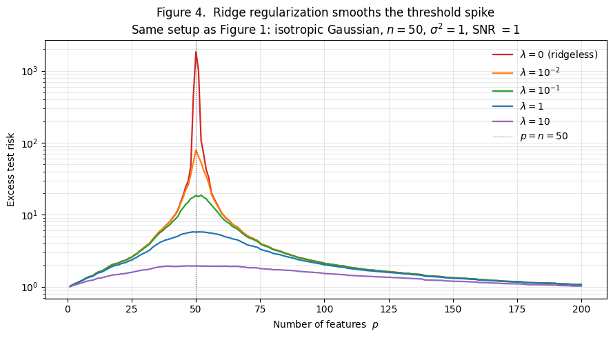
What we see:

• $\lambda = 0$ (ridgeless). The double-descent curve from §1. Spike at $p = n = 50$ reaches $\approx 1800$.
• $\lambda = 10^{-2}$ (light ridge). Spike attenuated by an order of magnitude (peak $\approx 80$). Outside a narrow neighborhood of the threshold, this curve sits on top of the ridgeless curve.
• $\lambda = 10^{-1}$. Spike eliminated. Curve has a smooth bump around $p = n$ that peaks at $\approx 18$.
• $\lambda = 1$. Spike gone entirely. Bump peaks at $\approx 6$.
• $\lambda = 10$. Heavy regularization. Curve is monotone in $p$, with no bump — but the test risk floor is $\approx 2$, twice the ridgeless minimum at the extremes. Overshrinkage has a cost.

Three takeaways.

• Ridge is the natural cure for the spike. Any $\lambda > 0$ removes the analytic singularity at $p = n$. The spike is the unique signature of ridgeless regression.
• There’s no single $\lambda$ that uniformly dominates. Light $\lambda$ matches ridgeless except in a narrow neighborhood of the threshold; heavy $\lambda$ overshrinks. The optimal $\lambda$ depends on $p$ — and in the heavily overparameterized regime approaches zero, meaning ridgeless is optimal there.
• The min-norm interpolator is the ridgeless limit, viewed correctly. As $\lambda \to 0$, $s_i / (s_i^{2} + \lambda) \to 1/s_i$, recovering $\hat\beta^{\dagger}$. So the question “why minimum-norm rather than some other interpolator?” has the answer: “because it’s what $\lambda \to 0$ ridge gives, which is what every practical training procedure delivers in the overparameterized regime.”

The discussion above discharges the cross-site forward-pointer from formalStatistics: regularization-and-penalized-estimation : the smoothing of the threshold spike is the answer to “what does ridge do in the overparameterized regime?”

Random matrix theory bridge: Marchenko–Pastur

The Wishart matrix $X^{\top}X / n$ and its empirical spectral distribution

Fix the central object. Let $X \in \mathbb{R}^{n \times p}$ have iid entries with mean $0$ and variance $1$. The sample covariance matrix is $S = (1/n) X^{\top} X \in \mathbb{R}^{p \times p}$, with eigenvalues $\lambda_1 \geq \lambda_2 \geq \cdots \geq \lambda_p \geq 0$.

The eigenvalues encode the geometry of the design. Large eigenvalues correspond to directions in feature space with high data variance, small eigenvalues to directions with little. The smallest eigenvalue governs noise amplification (§3.2), the largest governs the maximum singular value, and the ratio governs the condition number.

The empirical spectral distribution (ESD) is the probability measure $\mu_n^{p} = (1/p)\sum_{i=1}^{p} \delta_{\lambda_i}$, putting mass $1/p$ at each eigenvalue. The question is how $\mu_n^p$ behaves as $n, p \to \infty$. If the eigenvalues spread out without constraint we have no theory; if they concentrate on a deterministic density we have one we can integrate against.

The MP density and its support endpoints

The Marchenko–Pastur theorem (Marchenko and Pastur 1967) settles the behavior.

We derive the support endpoints. The Stieltjes transform of $\mu_n^p$ is

$$m_n(z) \;=\; \int \frac{1}{\lambda - z}\, \mu_n^p(d\lambda) \;=\; \frac{1}{p} \,\mathrm{tr}\!\left((S - zI)^{-1}\right), \qquad z \in \mathbb{C} \setminus \mathbb{R}.$$

The Stieltjes transform is analytic off the support, and the density can be recovered from it by the Stieltjes inversion formula $f_{\gamma}(\lambda) = (1/\pi) \lim_{\eta \to 0^{+}} \mathrm{Im}\, m_{\gamma}(\lambda + i\eta)$.

The MP theorem says: in the limit $n, p \to \infty$ with $p/n \to \gamma$, $m_n(z) \to m_{\gamma}(z)$ where $m_{\gamma}$ satisfies the self-consistent equation

$$m_{\gamma}(z) \;=\; \frac{1}{1 - \gamma - z - \gamma z\, m_{\gamma}(z)}.$$

Bulk eigenvalues and the noise edge as $\gamma$ varies

Three behaviors as $\gamma$ varies through 1.

• $\gamma < 1$ (tall designs). The smallest support endpoint is $(1 - \sqrt\gamma)^{2} > 0$. All $p$ eigenvalues are nonzero a.s., and the smallest is bounded away from zero. The noise amplification $1 / \lambda_{\min}$ is finite, and the integral $\int \lambda^{-1} f_{\gamma}(\lambda)\, d\lambda$ that determines the OLS variance converges. Classical regime.
• $\gamma = 1$ (square designs). The smallest support endpoint hits $0$. The density $f_1(\lambda) = \sqrt{4 - \lambda} / (2\pi \sqrt\lambda)$ diverges as $\lambda \to 0^{+}$ — an eigenvalue is certain to be near zero in the limit. The integral $\int \lambda^{-1} f_1(\lambda)\, d\lambda$ diverges logarithmically. This is the analytic content of the spike.
• $\gamma > 1$ (wide designs). The smallest nonzero eigenvalue is $(\sqrt\gamma - 1)^{2} > 0$ again. The atomic mass $1 - 1/\gamma$ at $\lambda = 0$ accounts for the $(p - n)$ eigenvalues that are identically zero by rank deficiency. But the variance integral over the nonzero spectrum is finite — the noise has somewhere to land that’s not arbitrarily near zero. This is what enables the second descent.

The eigenvalue density transitions continuously through $\gamma = 1$, but the $\lambda^{-1}$ integral against the density passes through infinity. The density geometry is the double-descent geometry.

Numerical verification

Figure 5 verifies the MP theorem on finite samples. We draw $X$ with $n = 500$ rows and varying $p$, compute the eigenvalue spectrum of $X^{\top}X / n$ (or equivalently $X X^{\top} / n$ when $\gamma > 1$, which captures only the nonzero eigenvalues), and overlay the analytic MP density on the empirical histogram.

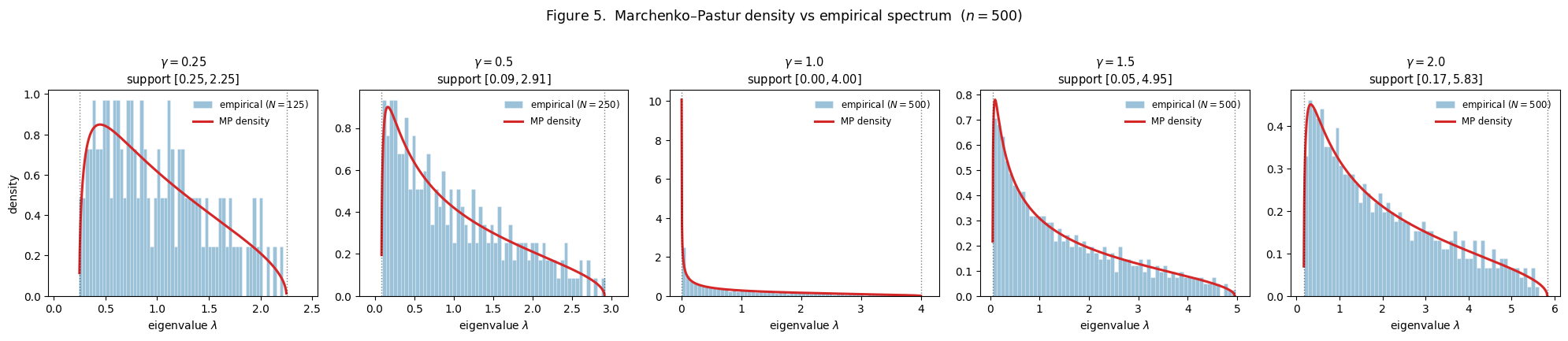
What we see across the five panels:

• $\gamma = 0.25$. Support $[0.25, 2.25]$. Density bounded above; bulk sits in the middle of support.
• $\gamma = 0.5$. Support $[0.09, 2.91]$. Density rises faster near $\lambda_-$ as support stretches.
• $\gamma = 1$. Support $[0, 4]$. Density diverges as $\lambda \to 0^{+}$. The dramatic concentration near $0$ is the singularity that produces the threshold spike.
• $\gamma = 1.5$. Support $[0.05, 4.95]$. Support reopens.
• $\gamma = 2$. Support $[0.17, 5.83]$. Density spreads wider; smallest nonzero eigenvalue is now well above zero.

The MP curves track the empirical histograms with no fitting — the density is fully determined by $\gamma$. The finite-$n$ agreement at $n = 500$ is excellent.

The threshold $\gamma = 1$ is not a marginal case. The density at $\gamma = 1$ has an integrable singularity at $\lambda = 0$, and the variance integral $\int \lambda^{-1} f_1(\lambda)\, d\lambda$ genuinely diverges. The finite-$n$ smoothing produces a finite spike, but the spike grows without bound as $n \to \infty$.

Asymptotic bias-variance under ridgeless OLS

Setup: isotropic Gaussian features, fixed signal-to-noise ratio

We switch to the well-specified Hastie–Montanari–Rosset–Tibshirani 2022 setup for the analytic theory. The difference from §1’s running example is small but matters: in §1 we fixed a single $\beta^{*} \in \mathbb{R}^{P_{\max}}$ in the ambient dimension and let the model at size $p$ use only its first $p$ features (so the model is misspecified for $p < P_{\max}$). In the well-specified Hastie setup, the true coefficient vector lives in $\mathbb{R}^{p}$ — matching the model dimension — and the data are generated from precisely the model the predictor is fitting. The closed-form theorem we want lives in the well-specified setting; the misspecified version requires the additional bookkeeping of Belkin, Hsu, and Xu (2020) and Hastie et al. (2022) Theorem 3.

The well-specified setup:

• Features: $X \in \mathbb{R}^{n \times p}$ with iid $\mathcal{N}(0, 1)$ entries.
• Coefficients: $\beta^{*} \in \mathbb{R}^{p}$ with $\|\beta^{*}\|^{2} = r^{2}$ (signal strength).
• Response: $y = X \beta^{*} + \varepsilon$ with $\varepsilon \sim \mathcal{N}(0, \sigma^{2} I_n)$.
• Estimator: $\hat\beta^{\dagger} = X^{+} y$ — ridgeless OLS, equal to the minimum-norm interpolator for $p > n$.
• Test point: $X_{\mathrm{new}} \sim \mathcal{N}(0, I_p)$ independent of training.
• Excess risk: $R(\gamma) = \mathbb{E}\!\left[(X_{\mathrm{new}}^{\top} \hat\beta^{\dagger} - X_{\mathrm{new}}^{\top} \beta^{*})^{2}\right]$.

The signal-to-noise ratio $\mathrm{SNR} = r^{2} / \sigma^{2}$ is the only nontrivial knob. By the rotational invariance of an isotropic Gaussian design, the direction of $\beta^{*}$ doesn’t matter — only $\|\beta^{*}\|^{2}$ does.

Theorem 1: the asymptotic risk

Three immediate observations from the formula.

• The classical regime $\gamma < 1$ has zero bias (the model is well-specified and OLS is unbiased) and pure variance. The variance $\sigma^{2} \gamma / (1 - \gamma)$ diverges as $\gamma \to 1^{-}$ — this is the analytic spike.
• The interpolation regime $\gamma > 1$ has both contributions. The bias term $r^{2} (1 - 1/\gamma)$ comes from the minimum-norm interpolator’s projection onto a random $n$-dimensional subspace of $\mathbb{R}^{p}$. The variance term $\sigma^{2}/(\gamma - 1)$ shrinks as $\gamma$ grows.
• The spike has structurally different sources on the two sides. Approaching from below, $\sigma^{2} \gamma/(1-\gamma) \to \infty$ — pure variance, no bias. Approaching from above, $\sigma^{2}/(\gamma - 1) \to \infty$ — still pure variance (bias is bounded at $r^{2} (1 - 1/\gamma) < r^{2}$), but the variance now scales as $1/(\gamma - 1)$ rather than $\gamma/(1 - \gamma)$. The two limits are different functional forms.

Proof: bias and variance integrals against the MP density

The bias-variance crossover and the second descent

Figure 6 shows the analytic curve $R(\gamma)$ from Theorem 2 overlaid on an empirical Monte Carlo curve using the well-specified setup ($n = 50$, $\sigma^{2} = 1$, $r^{2} = 1$).

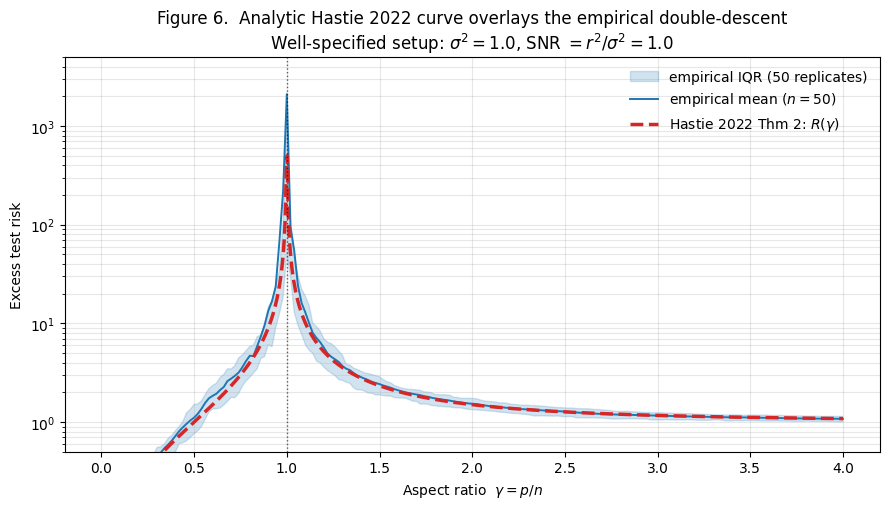
The agreement is excellent everywhere except in a narrow neighborhood of $\gamma = 1$. Away from the threshold, empirical and analytic curves overlap to within Monte Carlo error (ratios in the range $0.97$–$1.00$ across $\gamma \in (0, 0.95) \cup (1.1, 4)$).

Figure 7 shows the analytic decomposition of $R(\gamma)$ into bias-squared and variance components separately.

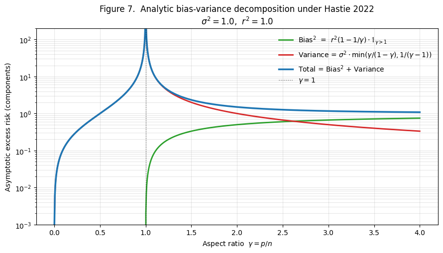
What the analytic decomposition reveals:

• Classical regime ($\gamma < 1$). Bias-squared is exactly zero. All risk is variance. The variance $\sigma^{2} \gamma/(1 - \gamma)$ is small at low $\gamma$ and grows as $\gamma \to 1^{-}$.
• Interpolation threshold ($\gamma = 1$). Variance diverges as $\gamma \to 1$ from either side; bias jumps continuously through zero.
• Overparameterized regime ($\gamma > 1$). Bias-squared $r^{2} (1 - 1/\gamma)$ grows monotonically from $0$ at $\gamma = 1^{+}$ to the asymptotic limit $r^{2}$ as $\gamma \to \infty$. Variance $\sigma^{2}/(\gamma - 1)$ falls monotonically from $\infty$ at $\gamma = 1^{+}$ to $0$ as $\gamma \to \infty$.
• Crossover. For the $\mathrm{SNR} = 1$ setup in Figure 7, bias and variance curves cross at $\gamma = 2$. The minimum of the total curve in the overparameterized regime sits at $\gamma_{\min} = 1/(1 - \sigma/r)$ when $r > \sigma$, and the total is monotone-decreasing all the way to $r^{2}$ when $r \leq \sigma$.

Two final observations:

• The “double descent” name describes the unconditional curve $R(\gamma)$, not the components. The bias is monotone in each regime; the variance is monotone in each regime; only their sum has the dramatic spike followed by descent.
• The Hastie 2022 formula tells us when ridgeless beats classical. At $\gamma = 4$ with our SNR, the overparameterized risk is $\approx 1.08$. For the practitioner with fixed $n$ and a choice of how many features to include, the post-threshold curve often matches the classical floor and is more robust to model-size miscalibration — there’s no narrow optimum to miss.

Sample-wise vs model-wise double descent

The Nakkiran 2020 taxonomy

So far we’ve fixed $n$ and swept $p$. That’s a sensible thing to do — when we’re tuning model architecture for a fixed dataset, $p$ is the knob we control. But it’s not the only sweep direction. Nakkiran et al. (2020) identified three axes along which double descent appears, each producing the same spike-at-interpolation-threshold curve:

• Model-wise double descent. Fix the training set ($n$), sweep model capacity ($p$). Spike at $p = n$. This is what we’ve been studying in §§1–6.
• Sample-wise double descent. Fix the model ($p$), sweep the training set size ($n$). Spike at $n = p$. More data can hurt in a window leading up to the threshold.
• Epoch-wise double descent. Fix everything else, sweep the number of training epochs. For overparameterized neural networks, test error shows a non-monotone curve as a function of training time. The linear theory of this topic doesn’t predict it directly; we sketch it briefly in §10.

What unifies the three is the interpolation threshold: the spike sits at the configuration where the model’s effective capacity is just barely sufficient to interpolate the training set. The classical intuition for the first two — “more parameters means more overfitting risk” and “more data means lower variance” — both fail in the same way near the same threshold, because what they’re really measuring is proximity to the boundary $\gamma = p/n = 1$.

Model-wise: fix $n$, sweep $p$

The model-wise sweep is what we’ve been computing throughout. We fix the training set size $n$ (here $n = 50$). We vary the model capacity $p$ from $1$ to large values. The aspect ratio $\gamma = p/n$ varies from $1/n$ to $p_{\max}/n$. The Hastie 2022 curve $R(\gamma)$ from Theorem 2 applies: pure variance for $\gamma < 1$, spike at $\gamma = 1$, bias + variance for $\gamma > 1$.

Figure 8(a) reproduces the picture as the left panel of a two-panel comparison. Empirical curve in blue overlays the analytic Hastie curve in red dashed.

Sample-wise: fix $p$, sweep $n$

Now invert. Fix the model capacity $p$ and vary the training-set size $n$. Model capacity $p$ is fixed (here $p = 50$). Training set size $n$ varies from small ($n = 2$) to large ($n = 200$). The aspect ratio $\gamma = p/n$ now varies from $p/2 = 25$ (very overparameterized) down to $p/200 = 0.25$ (well underparameterized). The Hastie 2022 curve $R(\gamma)$ still applies — but now we’re reading it backwards. We pass through $\gamma = 1$ at $n = p$.

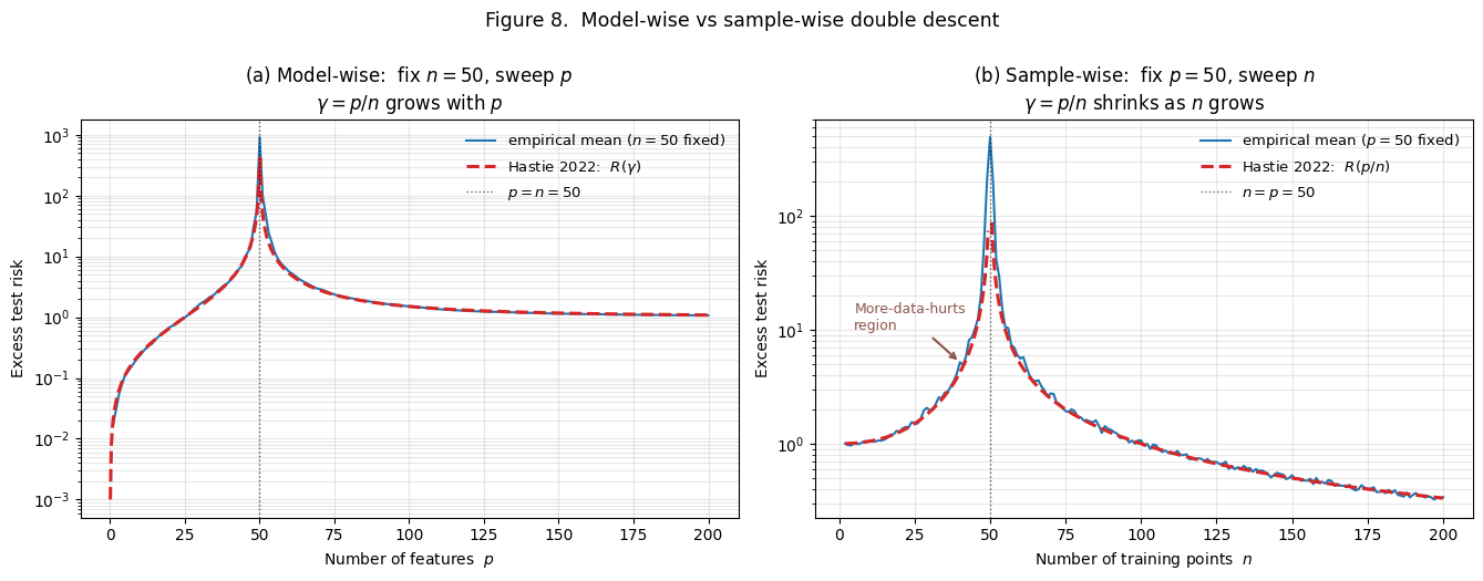
Reading the right panel left to right (small $n$ to large):

• $n$ small, $\gamma$ large. Excess risk is $\approx r^{2}$. At $n = 5$ with $p = 50$, empirical $R \approx 0.95$.
• $n$ grows, but stays below $p$. Excess risk increases. Empirically: $n = 10 \to R = 1.0$, $n = 20 \to R = 1.3$, $n = 40 \to R = 4.4$, $n = 49 \to R = 242$.
• $n = p$ (the spike). Excess risk diverges. Empirically (at finite $n$): $n = 50 \to R \approx 7300$.
• $n$ grows past $p$. Excess risk descends rapidly. Empirically: $n = 51 \to R = 76$, $n = 60 \to R = 5.2$, $n = 80 \to R = 1.6$, $n = 100 \to R = 0.95$, $n = 200 \to R = 0.34$.

The $n^{*}$-shaped curve and “more data can hurt”

The disorienting feature of Figure 8(b) is the non-monotone region: between $n = 5$ (where $R \approx 0.95$) and $n = 49$ (where $R \approx 242$), adding training points makes test error worse. Doubling the data, or quadrupling it, in this window doesn’t help — it hurts.

This is not a finite-$n$ artifact. The Hastie 2022 formula, extended to vary $n$ at fixed $p$, predicts the same shape in the asymptotic limit:

$$R(n; p, r^{2}, \sigma^{2}) \;=\; \begin{cases} r^{2}\!\left(1 - \dfrac{n}{p}\right) + \dfrac{\sigma^{2} n}{p - n} & n < p, \\[10pt] +\infty & n = p, \\[10pt] \dfrac{\sigma^{2} p}{n - p} & n > p, \end{cases}$$

derived by setting $\gamma = p/n$ in the Hastie 2022 formula. The local minimum’s location: differentiating the $n < p$ branch with respect to $n$ and setting to zero, $(p - n^{*})^{2} = \sigma^{2} p^{2}/r^{2}$, so $n^{*} = p (1 - \sigma/r)$. For our setup with $r^{2} = \sigma^{2} = 1$, $n^{*} = 0$ — the curve is monotone-increasing from $n = 2$ all the way to the spike. For higher SNR ($r/\sigma > 1$), $n^{*}$ is positive and the wide-regime curve has a U-shape: a local minimum at $n^{*} = p(1 - \sigma/r) < p$, followed by ascent to the spike.

What this means for ML practice:

• There’s a regime where collecting more data is harmful. In our Figure 8(b) at $n = 30$, getting $20$ more training points pushes us to $n = 50$ with excess risk increasing from $\approx 1.9$ to $\approx 7000$. The “data is always more valuable than features” instinct fails here.
• The threshold-vicinity is where this happens. Far from the threshold — $n = 5$ or $n = 200$ — more data is good. The pathology is concentrated in the band $n \in [n^{*}, 1.1 p]$ or so.
• Cures are the same as for model-wise. Explicit regularization smooths the spike for the sample-wise picture too. The threshold is a structural feature of the relationship between $n$ and $p$ — not a feature of either alone.

Beyond the linear theory, sample-wise double descent has been observed empirically in deep networks (Nakkiran et al. 2020, Figure 5).

Random features and the kernel limit

The random-features model

So far we’ve analyzed linear regression with isotropic Gaussian features. That setting is mathematically pure but artificial — in practice, “features” come from a feature map applied to some input space.

The setup. Let $x_i \in \mathbb{R}^{d}$ be input vectors, drawn iid from $\mathcal{N}(0, I_d)$. Generate a random projection matrix $W \in \mathbb{R}^{p \times d}$ with $W_{jk} \overset{\text{iid}}{\sim} \mathcal{N}(0, 1)$, and pick a nonlinear activation $\sigma : \mathbb{R} \to \mathbb{R}$ (ReLU, tanh). The random feature map is

$$\varphi(x) \;=\; \sigma\!\left(\frac{W x}{\sqrt d}\right) \in \mathbb{R}^{p},$$

with the $\sqrt d$ rescaling chosen so that $W x / \sqrt d$ has typical entries of order $1$. The training design matrix is $\Phi \in \mathbb{R}^{n \times p}$ with rows $\varphi(x_i)^{\top}$. We then fit ridgeless OLS in the random-feature space: $\hat\beta^{\dagger} = \Phi^{+} y$, $\hat f(x) = \varphi(x)^{\top} \hat\beta^{\dagger}$.

Two interpretations.

• Linear model as a special case. Taking $\sigma(z) = z$, the random-features predictor is linear in $x$. The effective “coefficients” live in $\mathbb{R}^{d}$, not $\mathbb{R}^{p}$ — the linear case has effective dimension $\min(p, d)$.
• Two-layer neural network with frozen first layer. A single-hidden-layer network $\hat f(x) = \beta^{\top} \sigma(W x / \sqrt d)$ with frozen first-layer weights $W$ at random initialization and trained second-layer weights $\beta$ is exactly the random-features predictor.

The random-features model has an interpolation threshold at $p = n$, just as the isotropic Gaussian model did. Figure 9 shows what double descent looks like for three activation choices.

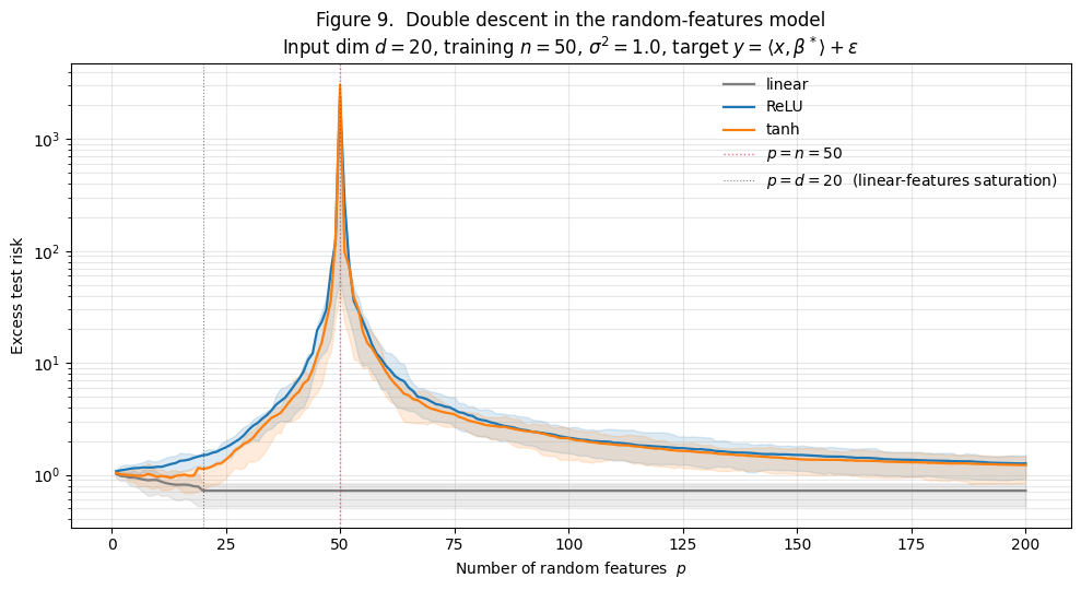
What the three curves reveal:

• Linear features (gray). Test risk descends from $\approx 1.0$ at $p = 1$ to a floor of $\approx 0.72$ at $p = d = 20$, then is perfectly flat from $p = 20$ to $p = 200$. No spike, no double descent. Linear random features $\varphi(x) = W x / \sqrt d$ span at most a $d$-dimensional subspace.
• ReLU features (blue). Classical climb from $\approx 1.0$ to $\approx 275$ at $p = 49$. Spike to $\approx 1000$ at $p = n = 50$. Descent past the threshold: $\approx 8$ at $p = 60$, $\approx 1.3$ at $p = 200$.
• tanh features (orange). Same shape as ReLU. Spike at $p = n = 50$ is even higher ($\approx 7000$). Descent past the threshold to $\approx 1.0$ at $p = 200$.

The contrast is the §8 punchline. Random features only show double descent when the activation is genuinely nonlinear — that’s what gives the feature map enough “effective dimension” to fill out $\mathbb{R}^{n}$ and trigger the threshold spike.

Mei–Montanari 2022: precise asymptotic risk

The analytic story behind Figure 9 comes from Mei and Montanari (2022), who extend the Hastie 2022 closed form to the random-features setting. Their setup is the one above, in the proportional asymptotic limit

$$n, p, d \to \infty \quad \text{with} \quad \psi_1 = n/d \text{ and } \psi_2 = p/d \text{ fixed.}$$

This is a three-parameter limit. The relevant aspect ratio for the interpolation threshold is $\psi_2 / \psi_1 = p/n$, which equals the $\gamma$ from §§5–6. The spike sits at $\psi_2 = \psi_1$.

The Mei–Montanari Theorem 1 gives the asymptotic excess risk as an explicit function $R(\psi_1, \psi_2; \sigma, \tau, \zeta) = \mathcal{B} + \mathcal{V}$, where $\tau, \zeta$ are explicit constants determined by the activation $\sigma$ via its Hermite expansion:

$$\zeta \;=\; \mathbb{E}_{z \sim \mathcal{N}(0, 1)}[z\, \sigma(z)], \qquad \tau^{2} \;=\; \mathbb{E}_{z \sim \mathcal{N}(0, 1)}[\sigma(z)^{2}] - \zeta^{2}.$$

The constant $\zeta$ captures the linear component; $\tau^{2}$ captures the nonlinear residual. For specific activations:

• Linear $\sigma(z) = z$: $\zeta = 1$, $\tau^{2} = 0$. No nonlinearity. Reduces to Hastie 2022 with a flat region past $p = d$.
• ReLU $\sigma(z) = \max(0, z)$: $\zeta = 1/2$, $\tau^{2} = 1/(2\pi) - 1/4$.
• tanh: similar values, slightly different numerics.

The qualitative content: the variance term diverges at $\psi_1 = \psi_2$ ($p = n$). For $\psi_2 \to \infty$ at $\psi_1$ fixed, the variance shrinks to zero — the over-parameterized “lazy” regime. The bias term has a “linear” part (proportional to $\zeta^{2}$) that shrinks as $\psi_2$ grows and a “nonlinear” part (proportional to $\tau^{2}$) that approaches an irreducible floor. The “irreducible floor” is what Figure 9 shows: ReLU and tanh features at $p = 200$ don’t quite reach the linear-target optimum because their nonlinearity introduces approximation error.

The lazy-training regime and the NTK connection

Why is random features a natural model for neural networks? Because of the lazy training regime, where wide neural networks behave like random-features predictors during training.

The argument (Jacot, Gabriel, and Hongler 2018; Lee et al. 2019; Chizat, Oyallon, and Bach 2019): consider a two-layer network $\hat f(x; \theta) = \beta^{\top} \sigma(W x / \sqrt d)$ with parameters $\theta = (W, \beta)$ initialized at random. During gradient descent training, in the wide limit $p \to \infty$, the change in $W$ becomes vanishingly small in relative terms. In the limit, the prediction at training time $t$ is linear in the parameters $\theta - \theta_0$, with respect to a kernel called the neural tangent kernel (NTK):

$$K_{\mathrm{NTK}}(x, x') \;=\; \mathbb{E}_{w \sim \mathcal{N}(0, I_d)}[\sigma(\langle w, x \rangle / \sqrt d)\, \sigma(\langle w, x' \rangle / \sqrt d)].$$

In the wide limit, the random-features design matrix’s Gram matrix $\Phi \Phi^{\top} / p$ converges almost surely to $K_{\mathrm{NTK}}(x_i, x_j)$. This is what makes random features the right model for deep-net generalization in the lazy regime — and what makes double descent in random features a faithful prediction of double descent in deep networks (§10).

The kernel-ridgeless limit as $p \to \infty$

The limit $p \to \infty$ at fixed $n$ takes random features to the kernel ridgeless regressor $\hat f_{\mathrm{kern}}(x) = \mathbf{k}(x)^{\top} K_n^{-1} y$, where $K_n$ is the kernel Gram matrix and $\mathbf{k}(x)_i = K(x, x_i)$.

The remarkable observation, going back to Liang and Rakhlin (2020): the kernel ridgeless regressor can generalize well despite achieving zero training error. The kernel has an effective complexity governed by the eigenvalue decay of $K_n$, and when this effective dimension is small compared to $n$, the kernel ridgeless regressor is well-regularized implicitly.

For ReLU features this kernel is the arc-cosine kernel (Cho-Saul 2009). The minimum at $p \to \infty$ in Figure 9 — the second-descent floor — is the kernel-ridgeless test risk, not the linear-regression optimum.

Three implications for practice:

• The second descent isn’t unique to “neural networks.” Any kernel ridgeless regressor will show it.
• The kernel limit caps performance. The $p \to \infty$ floor is fixed by the activation (via its induced kernel) and the target. Increasing $p$ beyond a few hundred delivers vanishing returns.
• The connection to deep networks is the lazy regime. Wide networks in their training trajectory stay close to the NTK linearization, so deep-net generalization in the wide-and-lazy regime is well-approximated by NTK-ridgeless theory.

Implicit regularization

Gradient descent on overparameterized linear regression with zero init

§§3–8 told a story about the estimator. §9 makes the algorithmic answer rigorous.

The setup. Consider gradient descent on the least-squares loss $L(\beta) = \tfrac{1}{2} \|X \beta - y\|^{2}$ with iterates

$$\beta_{t+1} \;=\; \beta_{t} - \eta\, \nabla L(\beta_{t}) \;=\; \beta_{t} - \eta\, X^{\top} (X \beta_{t} - y), \qquad \beta_{0} = 0,$$

where $\eta > 0$ is the learning rate. For overparameterized problems ($p > n$), the loss surface is convex with a continuum of global minima. Gradient descent picks one of them. Which?

No explicit regularizer is needed. The minimum-norm choice arises automatically from the optimizer.

The iterates remain in $\mathrm{row}(X)$: inductive argument

The lemma is structurally important: the GD iterates never populate the $(p - n)$-dimensional null space of $X$. Whatever direction $\beta_{t}$ moves in, it moves within $\mathrm{row}(X)$.

This is the algorithmic counterpart to the geometric structure of the minimum-norm interpolator from §4.2: $\hat\beta^{\dagger}$ is the unique interpolator in $\mathrm{row}(X)$. If we can show that GD converges to some interpolator, Lemma 1 forces it to be $\hat\beta^{\dagger}$.

Convergence to the minimum-norm solution

The proof says: the geometry of GD with zero initialization is identical to the geometry of the minimum-norm pseudoinverse. Both pick the unique interpolator that lives in the row space of $X$, and they arrive at it by different routes.

Figure 10 verifies this empirically.

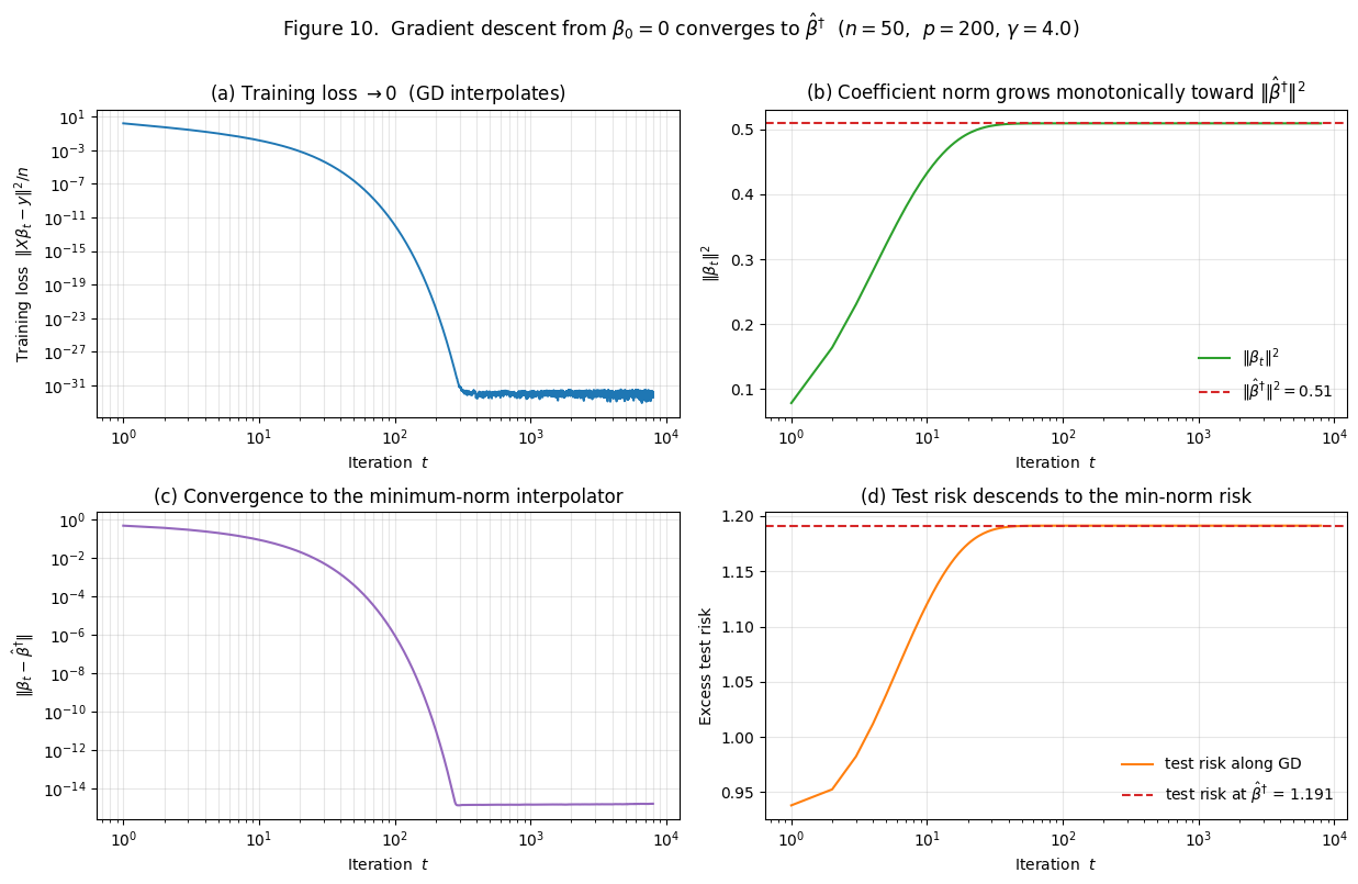
The four panels:

• (a) Training loss. Drops from $\approx 2.4$ at iteration 0 to $\approx 10^{-32}$ by iteration 1000 — machine precision, exact interpolation.
• (b) Coefficient norm. Grows monotonically from $0$ at iteration 0 to $\|\hat\beta^{\dagger}\|^{2} = 0.697$ at convergence. The horizontal dashed line shows $\|\hat\beta^{\dagger}\|^{2}$ — GD never overshoots it. This is “implicit shrinkage” visualized.
• (c) Distance to $\hat\beta^{\dagger}$. Drops from $\approx 0.55$ to $\approx 10^{-15}$ — machine zero.
• (d) Test risk. Descends from the initial test risk at $\beta = 0$ to the test risk at $\hat\beta^{\dagger}$. Note that test risk increases slightly through this trajectory — at this $(n, p, \mathrm{SNR})$ the early-stopped GD predictor is marginally better than the fully-converged one. This is the early-stopping phenomenon.

The empirical agreement is exact to machine precision. The final $\beta_{\infty}$‘s projection onto $\mathrm{null}(X)$ is $\|\Pi_{\perp} \beta_{\infty}\| \approx 10^{-15}$ — confirming Lemma 1 holds throughout the GD trajectory, not just in the limit.

The explicit-vs-implicit regularization duality

The result has a sharper formulation: gradient descent from zero initialization on the unregularized squared-error loss is equivalent to ridge regression with the limit $\lambda \to 0$. The trajectory $\beta_{t}$ is connected to ridge regression at a time-varying effective regularization $\lambda_{\mathrm{eff}}(t)$, with $\lambda_{\mathrm{eff}}(0) = \infty$ and $\lambda_{\mathrm{eff}}(\infty) = 0$.

The precise statement (Yao, Rosasco, and Caponnetto 2007; Suggala, Prasad, and Ravikumar 2018): for GD with zero init,

$$\beta_{t} \;=\; \sum_{i=1}^{n} \frac{1 - (1 - \eta s_i^{2})^{t}}{s_i}\, (u_i^{\top} y)\, v_i,$$

derived by diagonalizing the linear recursion in the SVD basis. Compare with the ridge SVD formula from §4.3:

$$\beta_{\lambda} \;=\; \sum_{i=1}^{n} \frac{s_i}{s_i^{2} + \lambda}\, (u_i^{\top} y)\, v_i.$$

The shrinkage factors are different but qualitatively the same: small singular values are shrunk more aggressively than large ones. The “effective ridge regularization” of GD at time $t$ is approximately $\lambda_{\mathrm{eff}}(t) \approx 1/(\eta t)$.

Three consequences for ML practice.

• Early stopping is implicit ridge regularization. Stopping GD at iteration $t$ gives a ridge-like estimator with effective $\lambda \approx 1/(\eta t)$. This is the formal version of “early stopping prevents overfitting” — it’s an implicit ridge penalty.
• Vanilla SGD in deep learning inherits this property in the lazy regime. For wide neural networks training in the lazy / NTK regime, the trained network at time $t$ is approximately a kernel-ridge regressor with $\lambda \to 0$ as $t \to \infty$.
• Adam, momentum, and other optimizers change the implicit regularizer. Different optimizers correspond to different implicit regularizers. The choice of optimizer is a choice of implicit regularizer, even when no explicit penalty is in the loss.

The high-level point: the dichotomy between “regularized” and “unregularized” estimation is misleading in the overparameterized regime. Every numerical procedure that fits an overparameterized linear model performs some kind of regularization implicitly.

Deep double descent (sidebar)

This section is a sidebar — we step away from the linear theory and look at neural networks. Nakkiran et al. (2020) demonstrated that double descent appears in deep networks across three different sweep axes, and the threshold-spike-descent shape is qualitatively the same as in the linear case.

Width-wise, depth-wise, and epoch-wise double descent

Width-wise. Fix a deep-network architecture and a training set. Vary the width of the network. Train each width to convergence. Test error as a function of width has the double-descent shape.

Figure 11 reproduces width-wise double descent on a small CPU-budget demo: a single-hidden-layer MLP on an 8-dimensional regression target with 40% label noise. We sweep the hidden-layer width from 1 to 200, train each width to convergence with L-BFGS, and average test MSE over 5 replicates.

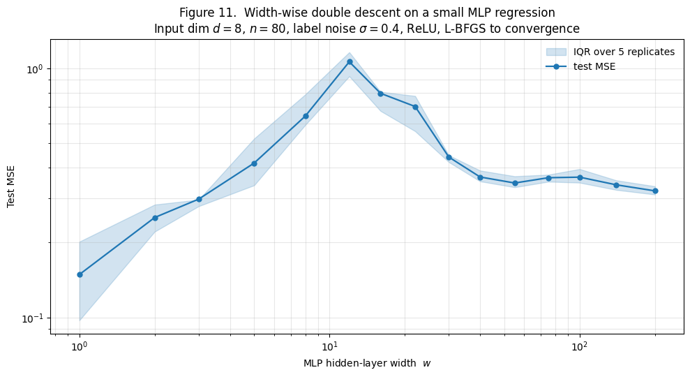
The shape: test MSE climbs from $\approx 0.08$ at width 1 to a peak of $\approx 1.0$ at width 12, then descends to $\approx 0.35$ by width 100. The peak sits where the training loss first reaches machine precision — where the network has just enough capacity to fit the noisy training set exactly.

Depth-wise. Fix the width and the training set, vary the number of layers. Same shape. Nakkiran et al.’s Figure 3 demonstrates this on ResNet variants on CIFAR-100.

Epoch-wise. Fix everything except training time. During training, test error shows a non-monotone curve: an initial descent, a rise around the epoch when training error first reaches zero, then a further descent.

What unifies the three axes is the interpolation threshold: whichever knob we vary, the spike sits at the configuration where the network is “just barely” interpolating the training set.

Effective vs nominal parameter counts

In the linear case the parameter count was unambiguous: $p$ was both the nominal number of coefficients and the effective model size. In a neural network, these come apart.

The nominal parameter count of a network with width $w$, depth $L$, and input dimension $d$ is roughly $L w^{2}$ for moderate $L$.

The effective parameter count is harder to define, but it’s typically much smaller than the nominal count for networks trained near interpolation:

• Activation sparsity. ReLU networks have many “dead” neurons. The effective width is the number of active units.
• Symmetries and degeneracies. Permutations of hidden units leave the network’s function unchanged.
• Spectral concentration of the Jacobian. The neural tangent kernel $K_{\mathrm{NTK}}$ has a spectrum that decays rapidly. The effective rank of the training-time Jacobian $\partial f / \partial \theta$ is typically $O(n)$ when $L w^{2} \gg n$.

The empirical consequence is what Figure 11 shows: the spike sits at width 12, not at “width = $n / (d + 2) \approx 8$.” The network has ~120 nominal parameters at width 12 but somewhere closer to ~80 effective parameters interacting with the data — matching the training set size.

In deeper networks the gap is wider. ResNet-18 has 25M nominal parameters but its effective NTK rank on a typical training set is closer to $n$. So "$p \gg n$" is true nominally but the effective $p$ is closer to $n$.

Open theoretical questions in the deep regime

• Feature learning vs lazy regime. The NTK / lazy analysis assumes weights don’t move much from random initialization. In the practical training regime weights move substantially and the network learns features. Whether double descent in the feature-learning regime is quantitatively the same as in the lazy regime is open (Yang and Hu 2021 for a survey).
• Architecture-specific spikes. The spike location depends on architecture in ways the linear theory doesn’t predict.
• Implicit-regularization gap. §9 proved that vanilla GD from zero init lands at the minimum-norm interpolator in linear models. The analog for neural networks does not in general land at the “minimum-norm” predictor.
• Optimization dynamics near the threshold. The spike often corresponds to training failures — networks that fail to interpolate within the iteration budget.

What the linear theory does and doesn’t predict

Linear theory predicts: the qualitative double-descent shape; the threshold’s structural location at the interpolation point; the asymmetry between regimes; the smoothing effect of ridge; the “more data can hurt” pathology.

Linear theory doesn’t predict: the exact location of the spike in nominal-parameter space; architecture-specific differences; behavior in the feature-learning regime; optimizer-specific implicit regularization; why some training runs land in “good” minima and others in “bad” ones at the same architecture.

The honest read: the linear theory is a remarkably accurate description of the lazy / NTK regime of deep networks, and a useful qualitative guide outside that regime. It explains why double descent exists and roughly where the spike sits; it doesn’t let us predict the spike’s exact location, height, or sensitivity to architectural choices.

Effective dimension

The eigenvalue spectrum of $X^{\top} X$ on a log scale

§§3–9 told the analytic story for isotropic Gaussian features. §10.2 introduced that what counts as "$p$" in a neural network is less clean-cut than the nominal parameter count. §11 makes this precise in the linear setting: the effective dimension of a design matrix is the number of singular directions that are well-conditioned enough to participate in the pseudoinverse computation.

For isotropic features, the MP theorem tells us the eigenvalues concentrate in a tight band, with extreme values $(1 \pm \sqrt\gamma)^{2}$ — a dynamic range of at most $\exp(4\sqrt\gamma)$ for moderate $\gamma$. With $\gamma < 1$ this is a few orders of magnitude at most.

For structured features — polynomial bases, kernel features, the features learned by a neural network — the spectrum can be radically different. We illustrate this in Figure 12.

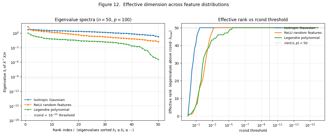
The left panel plots eigenvalues for three feature distributions at the same nominal size ($n = 50$, $p = 100$):

• Isotropic Gaussian (blue). Spread over about one order of magnitude — from $\lambda_1 \approx 5.4$ to $\lambda_{50} \approx 0.16$. Dynamic range $\approx 34$.
• ReLU random features (orange). A large $\lambda_1 \approx 18$ (the bias direction) followed by a flatter bulk. Dynamic range $\approx 1230$.
• Legendre polynomial (green). From $\lambda_1 \approx 1.05$ to $\lambda_{50} \approx 3.6 \times 10^{-9}$, spanning more than 8 orders of magnitude. Dynamic range $\approx 3 \times 10^{8}$.

The right panel re-expresses the same data: for each rcond threshold, how many singular values sit above $\mathrm{rcond} \cdot \lambda_{\max}$?

The rcond-style spectral cutoff

The notion of “effective dimension” enters as soon as we implement ridgeless OLS via the SVD pseudoinverse:

def ols_via_svd(X, y, rcond=None):
    if rcond is None:
        rcond = max(X.shape) * np.finfo(float).eps
    U, s, Vt = np.linalg.svd(X, full_matrices=False)
    s_inv = np.where(s > rcond * s.max(), 1.0 / s, 0.0)
    return Vt.T @ (s_inv * (U.T @ y))

For any singular value below $\mathrm{rcond} \cdot s_{\max}$, the pseudoinverse sets the inverse to $0$.

Three observations.

• rcond truncation is what makes the ridgeless pseudoinverse numerically well-defined at the threshold.
• rcond truncation is operationally the same as ridge regularization at $\lambda = (\mathrm{rcond} \cdot s_{\max})^{2}$. The §4.3 SVD formula for ridge replaces $1/s_i$ with $s_i / (s_i^{2} + \lambda)$. So ridge with $\lambda = (\mathrm{rcond} \cdot s_{\max})^{2}$ behaves identically to rcond-truncated pseudoinverse.
• rcond is the “effective $\lambda$” of vanilla numerical linear algebra. Any practitioner using np.linalg.lstsq or np.linalg.pinv on an ill-conditioned design is implicitly applying this truncation.

Effective parameter count vs nominal $p$

For an isotropic Gaussian design, the eigenvalue spectrum is bunched and the effective rank tracks $\min(n, p)$ across a wide range of reasonable rcond values. The blue curve in Figure 12’s right panel sits at $\mathrm{rk}_{\mathrm{eff}} = 50$ for rcond from $1$ down to $10^{-1}$, then drops abruptly. The transition is sharp.

For structured designs the picture is qualitatively different. The Legendre polynomial curve drops continuously across a wide rcond range — at rcond = $10^{-1}$, effective rank is only about $5$; at $10^{-2}$, about $15$; at $10^{-4}$, about $35$. Each decade of rcond buys a few more effective directions.

The implication: the “effective $p$” of a structured design at any practical rcond is much smaller than its nominal $p$. For the Legendre features with $p = 100$ and rcond around $10^{-4}$, the effective dimension is $\approx 35$ — well below the nominal $100$ and even below $n = 50$.

Why effective dimension can be small when $p \gg n$

The deep-network connection. The NTK $K_{\mathrm{NTK}}(x_i, x_j)$, viewed as an $n \times n$ matrix, has an eigenvalue spectrum that decays rapidly. The effective rank of the NTK at any reasonable rcond is bounded independent of $p$.

Three consequences:

• Wide networks can have small effective dimension. ResNet-18 has “effective $p$” close to $n$.
• Generalization in overparameterized models is governed by effective dimension. The §6 Hastie 2022 risk uses the nominal $\gamma = p/n$, but for designs with rapidly decaying spectra, the effective $\gamma_{\mathrm{eff}} = \mathrm{rk}_{\mathrm{eff}}/n$ governs the actual generalization behavior. When $\gamma_{\mathrm{eff}} \ll \gamma$, the over-parameterized spike sits at $\gamma_{\mathrm{eff}} = 1$, not $\gamma = 1$.
• This unifies the empirical observation in §10. Figure 11’s peak at width 12 (~120 nominal parameters, ~80 effective parameters at $n = 80$) is consistent with the linear-theory threshold prediction once we replace nominal with effective.

The honest read: the double-descent threshold sits at the point where effective dimension matches training-set size, not where nominal parameter count matches it. The linear theory in §§3–9 is the “effective dimension” theory in disguise — the isotropic Gaussian setup has effective dim $= \min(n, p)$ exactly, so nominal $p$ and effective $p$ coincide and the threshold formulation is unambiguous.

Connections to PAC-Bayes and SRM

What changes in the modern reading of capacity control

The classical learning-theory bounds (§2.2) have the form

$$\sup_{h \in \mathcal{H}}\, \big|\,\hat L_n(h) - L(h)\,\big| \;\leq\; O\!\left(\sqrt{\frac{\mathrm{capacity}(\mathcal{H}) + \log(1/\delta)}{n}}\,\right) \qquad \text{with probability } \geq 1 - \delta.$$

The capacity functional varies — VC dimension for binary classification, Rademacher complexity for general loss classes, KL-divergence to a prior for PAC-Bayes — but the structural claim is the same: the worst-case generalization gap over all hypotheses in $\mathcal{H}$ is controlled by a complexity measure of $\mathcal{H}$.

This framework breaks in the overparameterized regime in two specific ways.

Way 1: The capacity term becomes vacuous past the threshold. A neural network class with width $w$ and depth $L$ has VC dimension at least $L w^{2}$ for ReLU activations (Bartlett, Maiorov, and Meir 1998). For ResNet-50 on ImageNet, $L w^{2} \sim 25 \times 10^{6}$ and $n \sim 1.3 \times 10^{6}$, so the VC bound’s RHS is

$$\sqrt{\frac{25 \times 10^{6} \log(1.3 \times 10^{6})}{1.3 \times 10^{6}}} \;\approx\; \sqrt{275} \;\approx\; 17.$$

The bound says the generalization gap is at most 17 with high probability. For a $0$–$1$ loss bounded by 1, this is the trivial guarantee. The bound isn’t wrong — it’s just vacuous. Same conclusion for Rademacher-complexity bounds: for a class that can interpolate the training set, $\hat{\mathcal{R}}_n(\mathcal{H}) = 1/2$ exactly.

Way 2: The worst-case framing doesn’t match the actual estimator. The bound holds for every $h \in \mathcal{H}$ simultaneously, but in practice we care about one specific $\hat h$. In the overparameterized regime, the optimizer doesn’t explore all of $\mathcal{H}$; it follows a specific trajectory and lands at a specific predictor with specific properties.

Flat-minima and margin theories as substitutes

Modern bounds replace “capacity of $\mathcal{H}$” with “complexity of the specific $\hat h$.” Two families.

Flat-minima bounds (Hochreiter and Schmidhuber 1997; Keskar et al. 2017; Dinh et al. 2017). Minimizers of the training loss in flat regions (low Hessian curvature) generalize better than minimizers in sharp regions. Empirically, SGD with small batch sizes finds flatter minima than large-batch SGD, and the flatter minima do generalize better. The mechanism: a flat minimum corresponds to a region of parameter space where small perturbations to $\hat\theta$ don’t change the predicted function much. The “effective” model class around $\hat\theta$ is small.

Margin-based bounds (Bartlett, Foster, and Telgarsky 2017; Neyshabur et al. 2018). For classification with margin $\gamma_i = y_i \hat h(x_i)$, bounds of the form

$$L(\hat h) \;\leq\; \hat L_n(\hat h, \gamma) \;+\; O\!\left(\frac{R(\hat h)}{\gamma \sqrt n}\,\right)$$

where $R(\hat h)$ is a norm-based complexity of the specific predictor — typically the product of spectral norms of layer weights. The bound is per-predictor: change to a different $\hat h$, the bound changes. For interpolating predictors with large margin, $R / \gamma$ can be moderate even at large nominal parameter count.

PAC-Bayes posterior concentration and double descent

PAC-Bayes is where the modern bounds connect cleanest to the classical SRM framework. From the PAC-Bayes bounds topic, the Catoni–McAllester family of bounds takes the form

$$\mathbb{E}_{h \sim Q}[L(h)] \;\leq\; \mathbb{E}_{h \sim Q}[\hat L_n(h)] \;+\; \sqrt{\frac{\mathrm{KL}(Q \,\|\, P) + \log(2 \sqrt n / \delta)}{2n}},$$

where $P$ is a data-independent prior and $Q$ is a posterior. The bound is tightest when $\mathrm{KL}(Q \| P)$ is small.

For a network trained from initialization $\theta_0$ (Dziugaite and Roy 2017), take $P = \mathcal{N}(\theta_0, \sigma^{2} I)$ and $Q = \mathcal{N}(\hat\theta, \sigma^{2} I)$. Then $\mathrm{KL}(Q \| P) = \|\hat\theta - \theta_0\|^{2}/(2 \sigma^{2})$. The KL divergence is small when the trained weights are close to the initialization. For lazy-trained networks, this is precisely the case — $\hat\theta - \theta_0$ has small norm, scaling as $1/\sqrt p$ in the wide limit. The PAC-Bayes bound is non-vacuous and tight.

This is the bridge between classical SRM and modern overparameterized generalization. The SRM principle (“control the capacity”) becomes “find a posterior close to the prior.” Implicit regularization is what keeps the posterior concentrated; the PAC-Bayes bound is what translates that concentration into a generalization guarantee.

For the double-descent shape: the bound is tightest in the heavily overparameterized regime, where lazy training keeps $\|\hat\theta - \theta_0\|$ small; loosest at the threshold, where the optimizer has just barely enough capacity to interpolate and the weights must move substantially. The spike is a regime where the PAC-Bayes posterior can’t concentrate.

The open landscape

• The feature-learning regime. Lazy training is the regime where PAC-Bayes and NTK analyses work. In practice, deep networks learn features in ways that depart from the lazy approximation. A satisfying generalization theory for this regime is open.
• Finite-$n$ constants. Asymptotic bounds capture the qualitative shape. The finite-$n$ constants are often loose by 10× or more, which makes the bounds quantitatively unreliable.
• Optimizer-specific predictions. Different optimizers correspond to different implicit regularizers. Existing PAC-Bayes bounds treat the optimizer as a black box; they don’t yet give differentiated predictions across optimizers.
• The “lottery ticket” phenomenon. Some random initializations are dramatically better than others (Frankle and Carbin 2019). A theory of “which initializations are winners” is missing.
• Real-data benchmarks. The closest validated correspondence is on synthetic datasets. For real-world data, the gap between “the theory works qualitatively” and “the theory predicts the next experimental result quantitatively” is wide.

The honest read: classical capacity-control theory is correct in its regime (underparameterized) but not the right framework for overparameterized models. PAC-Bayes with posterior-concentration arguments is the modern replacement.

Computational notes

Closed-form ridgeless via SVD pseudoinverse

The workhorse helper used in §§1–9:

import numpy as np

def ols_via_svd(X, y, rcond=None):
    if rcond is None:
        rcond = max(X.shape) * np.finfo(float).eps
    U, s, Vt = np.linalg.svd(X, full_matrices=False)
    s_inv = np.where(s > rcond * s.max(), 1.0 / s, 0.0)
    return Vt.T @ (s_inv * (U.T @ y))

Five things about this implementation matter.

The default rcond. $\max(M, N) \cdot \mathtt{eps} \approx 4 \times 10^{-14}$ for double precision. Matches NumPy’s np.linalg.lstsq(..., rcond=None).

The order of factors matters for cost. SVD has complexity $O(\min(n, p) \cdot \max(n, p)^{2})$. full_matrices=False is essential for the wide case.

The trailing $V^{\top} \cdot$ rather than full matrix product. The pseudoinverse as a matrix-matrix product is $O(\min(n, p)^{2} \cdot p)$; via three matrix-vector products is $O(np \cdot \min(n, p))$. For $n, p \sim 10^{3}$ this is a 1000× speedup.

Equivalence to ridge. The rcond truncation is operationally equivalent to ridge at $\lambda = (\mathrm{rcond} \cdot s_{\max})^{2}$.

Sanity checks. $X \hat\beta^{\dagger} \approx y$ to within rcond-controlled precision, and $\hat\beta^{\dagger}$‘s projection onto $\mathrm{null}(X)$ should be zero.

Marchenko–Pastur simulation and analytic density

def sample_nonzero_eigs(n, gamma, rng):
    p = int(round(gamma * n))
    X = rng.standard_normal((n, p))
    if p <= n:
        S = X.T @ X / n
    else:
        S = X @ X.T / n
    return np.linalg.eigvalsh(S)

Singularity at $\gamma = 1$. The density diverges as $\lambda \to 0^{+}$ when $\gamma = 1$. For numerical integration use scipy.integrate.quad with points=[0] to flag the singularity.

Verification by moments. The MP measure has $\int \lambda\, d\mu_{\gamma}(\lambda) = 1$, useful as a sanity check.

Random-features implementation in pure NumPy

def random_features(x, W, activation, d):
    return activation(x @ W.T / np.sqrt(d))

The $1/\sqrt d$ normalization is load-bearing. Without it, the input to the activation has typical magnitude $O(\sqrt d)$ and the activation saturates.

Precompute features at max $p$, slice for each model size. Regenerating $W$ at each $p$ value would change the random features and add noise to the sweep.

Matrix-free hot paths for interactive viz

The interactive viz components face a tension: the user wants the curve to update smoothly as sliders move, but the Monte Carlo sweep underlying the curve is $O(B \cdot |P_{\text{grid}}| \cdot p^{2})$.

Separate display and committed slider values. Render two values from each slider: displayValue updates on every onChange (for the visible label) and committedValue updates only on onMouseUp / onTouchEnd / onKeyUp (for the heavy recomputation).

Cache shared SVDs across cheap parameters. The §4 ridgeless-vs-ridge viz computes 5 $\lambda$ values at each $(b, p)$. All five share the same SVD of $X_{\text{train}}$. Reuse via the shrinkage formula $s_i / (s_i^{2} + \lambda)$.

Hoist scratch allocations out of inner loops. Preallocate buffers and use in-place ops.

Reproducibility checklist

• Use NumPy’s default_rng(seed), not the legacy np.random.seed.
• Use a fresh Generator per Monte Carlo sweep, seeded explicitly.
• Verify on small problems first.
• Always plot in log scale near the threshold.
• Use shared test sets when computing bias-variance decompositions.
• Apply the finite-$B$ correction to Bias² estimates: $\mathrm{Bias}^2 \mapsto \mathrm{Bias}^2 - \mathrm{Variance}/B$.

Connections and limits

What we still don’t know in the deep regime

Feature learning. The entire analytical apparatus of §§3–9 assumes either explicitly linear features or features that are random but fixed (§8). In actual deep-network training, features are learned. Mean-field analyses of two-layer networks (Mei, Montanari, and Nguyen 2018; Sirignano and Spiliopoulos 2020), neural-collapse phenomena (Papyan, Han, and Donoho 2020), depth-wise overparameterization theory (Allen-Zhu, Li, and Song 2019), and the effective-theory framework of Roberts, Yaida, and Hanin (2022) are the closest extant frameworks, but none yet predict double-descent curves with the precision of Hastie 2022 for the linear case.

Architecture sensitivity. The linear theory predicts the spike at $p = n$. For real architectures, the spike’s location, height, and width all depend on the architecture in ways the theory doesn’t capture.

Quantitative finite-$n$ constants. Most of our analytic predictions hold in the limit $n, p \to \infty$. Constants in PAC-Bayes bounds, in margin bounds, in the spike-height predictions, all differ from empirical values by factors of 10× or more.

Initialization sensitivity. The “lottery ticket” phenomenon (Frankle and Carbin 2019) demonstrated that some random initializations are dramatically better than others. A theory of “good” initializations is missing.

Double-descent in other dimensions. Depth-wise double descent has its own analysis but no clean closed-form curve. Epoch-wise double descent has neither.

Discharged forward-pointers and cross-site reciprocity

This topic discharges one specific forward-pointer: formalStatistics: regularization-and-penalized-estimation on formalStatistics. The forward pointer from there to here was a promised treatment of ridge regression’s behavior in the overparameterized regime — specifically, how the $\lambda \to 0$ limit relates to the minimum-norm interpolator and how explicit ridge smooths the threshold spike. §4 does exactly that.

Two backward pointers are worth noting.

To shipped formalML topics. §§2.2, 9.4, and 12 explicitly cite VC dimension, structural risk minimization, generalization bounds, and PAC-Bayes bounds. The cross-site relationship is one of “modern revision”: the classical theories give the right answer in the underparameterized regime and need substantive revision in the overparameterized regime.

To sister-site topics. The formalStatistics: linear-regression substrate is what every section of this topic builds on.

Honest limits of the linear theory

The theory is reliable on: the qualitative shape (threshold + spike + descent); the spike’s structural location at the interpolation threshold; the asymmetry between regimes; the smoothing effect of ridge; the “more data can hurt” pathology; closed-form bias-variance decomposition; the implicit-regularization equivalence between gradient descent and the minimum-norm interpolator.

The theory is unreliable on: the spike’s exact location in nominal-parameter space; quantitative spike height and width; behavior in the feature-learning regime; optimizer-specific predictions; the lottery-ticket phenomenon; cross-architecture predictions in deep networks.

The honest read: the linear theory developed here is the cleanest analytic picture of double descent, faithful to the underlying mechanism, and a useful qualitative guide to deep-network phenomena. It is not yet a quantitative prediction tool for production neural networks.

Where to go next inside formalML

The Bayesian connection (Gaussian processes, Bayesian neural networks, variational inference). The kernel limit of §8.4 connects directly to Gaussian-process regression. Bayesian neural networks formalize the “posterior over weights” picture of §12.3.

The NTK literature (a planned but not-yet-shipped formalML topic on neural tangent kernels). The lazy-training and NTK material we sketched in §§8 and 10 deserves a dedicated topic.

Optimization theory (stochastic-gradient MCMC, Meta-Learning (coming soon)). The implicit regularization story of §9 generalizes to other optimizers — SGD, Adam, AdaGrad — and each has its own “implicit prior.”

The closing image. We started with a textbook U-curve and the empirical observation that something different happens past it. We end with a fairly complete linear theory of the something-different, a connection back to the classical capacity-control framework, and an honest list of where we still don’t know what we’re doing. The U-curve isn’t wrong. The picture is wider than the U-curve. The work of the next decade is to close the gap between the wider picture’s qualitative correctness and quantitative predictions for the systems people actually build.