Structural Risk Minimization

Motivation: why capacity control matters

The fixed-class ERM trap

Empirical risk minimization (ERM) — picking the hypothesis $\hat h \in \mathcal{H}$ that minimizes training error — is the foundational learning algorithm, and it behaves as advertised as long as the class $\mathcal{H}$ is small enough that uniform convergence kicks in (the Fundamental Theorem of Statistical Learning from PAC Learning is the formal statement). But small enough is doing all the work. If $\mathcal{H}$ is too small, we can’t represent the regression function well and bias dominates. If $\mathcal{H}$ is too rich, we fit the noise and variance dominates. The whole game in learning theory is navigating this trade-off, and the irritating fact is that we can’t navigate it by choosing $\mathcal{H}$ upfront: the best class to run ERM on depends on the data we haven’t seen yet — the sample size, the noise level, the smoothness of the target.

Make this concrete. Fit polynomials to $n = 50$ noisy points drawn from $m(x) = \sin(\pi x)$. Degree-1 polynomials underfit; they can’t bend. Degree-15 polynomials interpolate the noise and oscillate wildly between data points. Somewhere in between is a degree that captures the smooth structure without chasing the wiggles. ERM on $\mathcal{H}_1$ gives us a bad linear fit; ERM on $\mathcal{H}_{15}$ gives us a wild oscillator. ERM is the wrong question. The right question is which class $\mathcal{H}_k$ should we run ERM on?

Bias and variance as functions of capacity

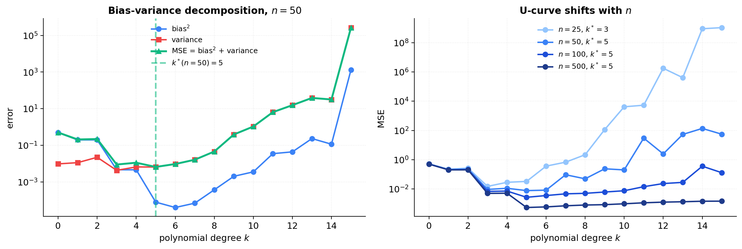
Fix a regression target $m: \mathcal{X} \to \mathbb{R}$ and a noise process $Y = m(X) + \varepsilon$ with $\mathbb{E}[\varepsilon] = 0$ and $\mathrm{Var}(\varepsilon) = \sigma^2$. For a nested sequence of classes $\mathcal{H}_1 \subset \mathcal{H}_2 \subset \cdots$, let $\hat h_k$ be the ERM in $\mathcal{H}_k$ on a sample of size $n$. The pointwise mean-squared test error against a fresh $Y' = m(x) + \varepsilon'$ decomposes as the usual bias-variance identity (see formalStatistics: linear-regression for the parametric derivation):

$$\mathbb{E}\left[(\hat h_k(x) - Y')^2\right] = \underbrace{\bigl(\mathbb{E}[\hat h_k(x)] - m(x)\bigr)^2}_{\text{bias}^2(k, x)} + \underbrace{\mathrm{Var}(\hat h_k(x))}_{\text{variance}(k, x)} + \sigma^2,$$

where the expectation is over the training sample $S \sim D^n$ and the fresh noise $\varepsilon'$, and $\sigma^2$ is the irreducible noise floor. The error against the regression function alone — $\mathbb{E}[(\hat h_k(x) - m(x))^2]$ — drops the $\sigma^2$ term and is just bias$^2(k, x) +$ variance$(k, x)$. Two observations carry the section. Bias is monotone non-increasing in $k$: a larger nested class can only approximate $m$ at least as well as a smaller one. Variance is monotone non-decreasing in $k$: a richer class has more freedom to chase noise, so $\hat h_k$ moves around more across resamplings of $S$. Add them and integrate over $x$ to get the expected MSE; the result is a U-curve in $k$.

The minimum of that U-curve — the true optimal $k^*(n)$ — is what we’d pick if we could see the population. The problem is that we can’t; the training error $\hat L_n(\hat h_k)$ is monotone non-increasing in $k$ (more flexibility never hurts in-sample) and bottoms out at zero by interpolation once $k$ is large enough. Empirical risk alone tells us a strictly wrong story about how to pick $k$.

Why the “true” optimal capacity depends on $n$

The U-curve isn’t fixed; it shifts with $n$. For ordinary least squares with $k+1$ parameters, the variance term at degree $k$ scales like $\sigma^2 (k+1) / n$ — the textbook Gauss–Markov consequence ( formalStatistics: linear-regression derives it). Doubling $n$ halves the variance contribution without touching the bias, so the U-curve flattens on the right and the optimum $k^*(n)$ shifts up: with more data, we can afford more complexity.

This is the central reason no fixed choice of $\mathcal{H}$ works across problem sizes. A degree-3 ERM that’s near-optimal at $n = 50$ leaves bias on the table at $n = 500$; a degree-9 ERM that’s near-optimal at $n = 500$ overfits catastrophically at $n = 50$. The optimal capacity is a function of $n$, so the model class itself has to be chosen as a function of the data.

SRM in one paragraph: penalize-and-pick

Structural Risk Minimization (SRM) is the recipe for choosing $\mathcal{H}_k$ from data. (1) Fix in advance a nested family $\mathcal{H}_1 \subset \mathcal{H}_2 \subset \cdots$, ordered by increasing capacity. (2) For each $\mathcal{H}_k$, define a capacity-dependent penalty $\mathrm{pen}(\mathcal{H}_k, n, \delta)$ that grows with the capacity of $\mathcal{H}_k$ and shrinks with $n$. (3) Pick the class $\hat k$ that minimizes training error plus penalty, and return $\hat h_{\hat k}$, the ERM on $\mathcal{H}_{\hat k}$:

$$\hat k \in \arg\min_{k \ge 1} \left\{\hat L_n(\hat h_k) + \mathrm{pen}(\mathcal{H}_k, n, \delta)\right\}, \qquad \hat h_{\hat k} = \arg\min_{h \in \mathcal{H}_{\hat k}} \hat L_n(h).$$

The penalty plays the role of a stand-in for the (unobservable) variance. When it’s calibrated correctly — meaning the penalty upper-bounds the gap $L(\hat h_k) - \hat L_n(\hat h_k)$ with probability $\ge 1 - \delta$ uniformly across $k$ — the picked class $\hat k$ provably tracks $k^*(n)$ as $n$ grows. The rest of this topic is about how to calibrate the penalty (VC dimension in §4, Rademacher complexity in §5, PAC-Bayes in §9) and what the trade-offs are.

n (sample size): 50σ (noise std): 0.20B (MC replicates): 100

At (n = 50, σ = 0.20, B = 100), the bias-variance optimum is k* = 5. Right panel: shifting n shifts k* rightward, the central claim of §1.3.

The nested-family setup

Definition: nested hypothesis-class family

A nested hypothesis-class family is a sequence $\mathcal{H}_1 \subset \mathcal{H}_2 \subset \cdots$ of hypothesis classes indexed by $k \in \mathbb{N}$, satisfying two conditions: nesting ($\mathcal{H}_j \subseteq \mathcal{H}_k$ whenever $j \le k$), and capacity monotonicity (a capacity functional $C: \{\mathcal{H}_k\} \to \mathbb{R}_{\ge 0}$ — VC dimension, Rademacher complexity, or effective degrees of freedom — non-decreasing in $k$ with $C(\mathcal{H}_k) \to \infty$).

SRM never runs ERM on $\mathcal{H}_\infty$; it always runs it on a finite class $\mathcal{H}_{\hat k}$ chosen from the family. Older Russian-school literature (Vapnik 1995) calls a nested family a filtration of the ambient class; the word is borrowed from probability theory and refers to the same object.

The indexing doesn’t have to be discrete — continuous-parameter families like RKHS norm balls $\mathcal{H}_r = \{f \in \mathcal{H}_K : \|f\|_K \le r\}$ are nested in $r$ and admit the same SRM analysis; this is the soft-SRM view we’ll formalize in §6. The choice of which nested family to use is a structural modeling decision that happens before seeing the data — the analog of choosing a parametric model in classical statistics. SRM picks $\hat k$ from the family, not the family itself. Picking the family poorly is a different (and unaddressed) failure mode.

Canonical examples

Four families recur throughout the topic and across the broader ML literature.

Polynomials by degree. $\mathcal{H}_k = \{p: [-1, 1] \to \mathbb{R} \mid \deg p \le k\}$, the toy from §1. The capacity is $C(\mathcal{H}_k) = k + 1$ — the dimension of the parameter space; for the threshold-classification variant of the same family, the VC dimension is also $k + 1$. This is the example we’ll use for all numerics through §11.

SVMs by inverse margin. $\mathcal{H}_\gamma = \{h \mid h(x) = \mathrm{sign}(\langle w, x \rangle + b),\ \|w\| \le 1/\gamma\}$, the large-margin family from Vapnik (1995). Larger $\gamma$ means a smaller class — the linear classifiers are restricted to those that separate with margin at least $\gamma$. Capacity scales as $1/\gamma^2$ for the worst-case Rademacher bound, independent of input dimension. This is the celebrated dimension-free property that motivates kernel methods, and it anchors §12.1.

Neural networks by width. $\mathcal{H}_w = \{\text{depth-}L \text{ feedforward nets with} \le w \text{ neurons per layer}\}$. The nesting is honest — a width-$w$ net is a special case of a width-$(w+1)$ net by zeroing out the last neuron — but the classical capacity measures are loose enough that the SRM bound is uninformative for any realistic deep net. This is the family where classical theory breaks (§12.2–12.4) and where implicit regularization takes over.

RKHS norm balls. For a reproducing-kernel Hilbert space $\mathcal{H}_K$ with kernel $K$, the family $\mathcal{H}_r = \{f \in \mathcal{H}_K : \|f\|_K \le r\}$ is nested in $r$, with empirical Rademacher complexity $\hat{\mathfrak{R}}_n(\mathcal{H}_r) \le r \sqrt{\sum_i K(x_i, x_i)}\,/n$ (Bartlett and Mendelson 2002). The squared-norm penalty $\lambda \|f\|_K^2$ implements SRM on $\{\mathcal{H}_r\}_{r \ge 0}$ in soft form — the §7.1 connection.

Others fit the same template — decision trees by depth (with pruning), boosted ensembles by round count, sparse linear models by $\ell_0$-norm. The unifying picture is an indexed family of classes, monotone in some capacity functional, with the index $k$ the free parameter the algorithm gets to set.

Capacity measures: VC dimension, Rademacher complexity, effective DoF

Different SRM bounds need different capacity functionals. Three are standard, and the choice between them in a specific bound has both theoretical and practical consequences.

VC dimension ($\dim_{\mathrm{VC}}(\mathcal{H})$). For binary classification, defined as the size of the largest set $\mathcal{H}$ can shatter — fully developed in VC Dimension and introduced in PAC Learning. VC dimension is a distribution-free, worst-case measure: it captures the largest possible generalization gap over all data-generating distributions. The Vapnik-style SRM bound (§4) uses VC dimension — universal but typically loose.

Rademacher complexity ($\hat{\mathfrak{R}}_n(\mathcal{H})$, $\mathfrak{R}_n(\mathcal{H})$). Defined as $\hat{\mathfrak{R}}_n(\mathcal{H}) = \mathbb{E}_{\sigma}[\sup_{h \in \mathcal{H}} \tfrac{1}{n}\sum_{i=1}^n \sigma_i h(x_i)]$ where $\sigma_i$ are i.i.d. Rademacher (uniform on $\{\pm 1\}$); the population version takes a further expectation over $X$ (Generalization Bounds). Rademacher complexity is distribution-dependent — it sees the actual training sample — and is typically sharper than VC dimension when $\mathcal{H}$ doesn’t shatter the data the distribution puts mass on. The Bartlett–Mendelson SRM bound (§5) uses it.

Effective degrees of freedom. For linear smoothers $\hat Y = S Y$ — least squares, ridge, kernel smoothers — the effective DoF is $\mathrm{tr}(S)$. For ordinary least squares with $k+1$ parameters this equals $k+1$ exactly; for ridge regression with penalty $\lambda$ it’s $\mathrm{tr}(\mathbf{X}(\mathbf{X}^\top \mathbf{X} + \lambda \mathbf{I})^{-1} \mathbf{X}^\top)$, which is strictly less than $k+1$ for $\lambda > 0$ and decreases as $\lambda$ grows. Effective DoF is the capacity functional underlying AIC, BIC, and the SRM-as-regularization story in §7; it’s specific to linear or near-linear estimators but is the practitioner’s everyday measure.

The three are related but not interchangeable. For a class of VC dimension $d$, the worst-case Rademacher complexity satisfies $\mathfrak{R}_n(\mathcal{H}) = O(\sqrt{d \log n / n})$ — a Sauer–Shelah consequence. For our polynomial-regression toy, all three measures grow linearly in $k$, which is why the same SRM picture works regardless of which one we use. For richer model classes — especially deep nets — they diverge sharply, which is part of §12’s story.

What goes wrong with non-nested families

Some natural model families aren’t nested. The clean example is $k$-nearest neighbors: the class $\mathcal{H}_k^{kNN}$ of $k$-NN rules indexed by neighbor count is not nested under inclusion — a 3-NN rule is not a special case of a 5-NN rule. Decision trees indexed by depth are nested under pruning; trees indexed by leaf count typically are not. SVMs with different kernels (linear, RBF, polynomial) form a discrete unordered set, not a chain.

The fix is to drop the literal-inclusion requirement and keep only the capacity-indexed part. Given any countable indexed family $\{\mathcal{H}_k\}_{k \ge 1}$ with capacity $C_k$ monotone non-decreasing, the union-bound argument that produces the SRM penalty (§3) goes through unchanged — we never actually used $\mathcal{H}_j \subset \mathcal{H}_k$ in the derivation, only that we’d allocated a per-class confidence budget $\delta_k$ with $\sum_k \delta_k \le \delta$. The same SRM estimator $\hat k = \arg\min_k \{\hat L_n(\hat h_k) + \mathrm{pen}(\mathcal{H}_k)\}$ is well-defined, and the same oracle inequality (§3.3) holds with the same proof.

In Vapnik’s original formulation the families are nested for cleanliness, but everything generalizes to a capacity-indexed sequence (Shawe-Taylor et al. 1998 treat the data-dependent and non-nested cases explicitly). The cost of relaxing nesting is interpretive, not formal: the bias term doesn’t decompose monotonically when classes overlap unpredictably, so the “more data lets us afford more capacity” story becomes less crisp. For most practical applications — degree-indexed polynomials, depth-indexed trees, width-indexed nets, $C$-indexed SVMs — the families are nested and the cleaner version applies.

Visualizing the polynomial ladder

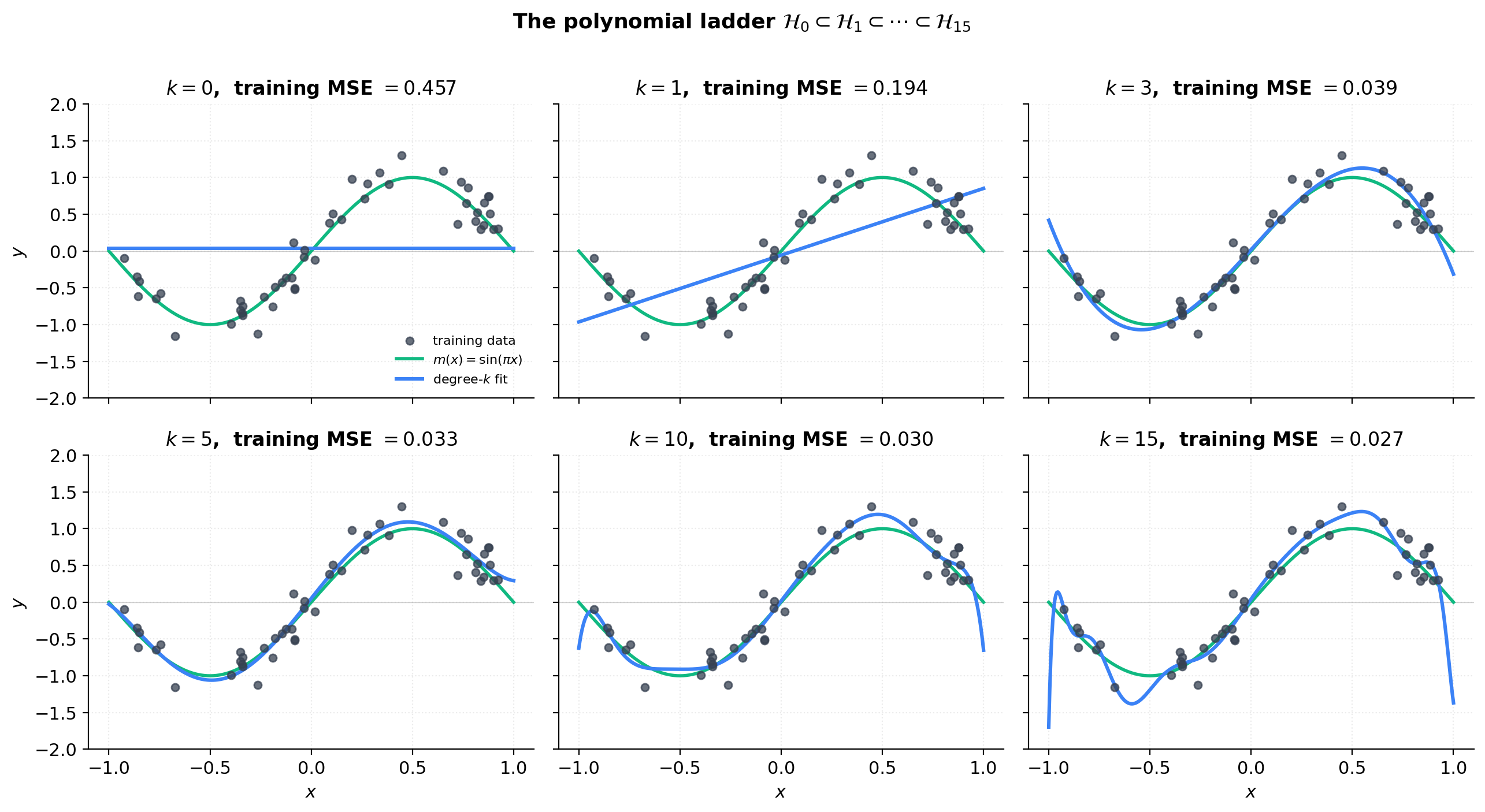
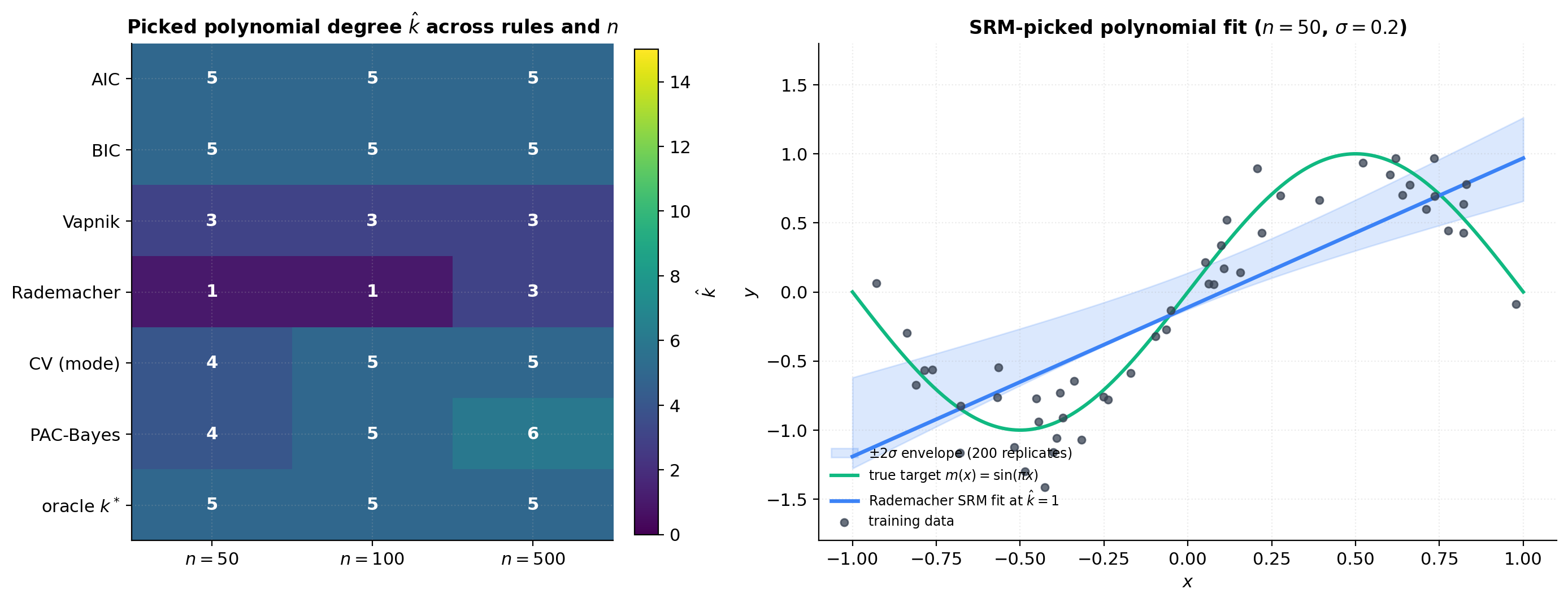
The figure below makes the nested family concrete. On a single training sample of $n = 50$ from the §1 toy, we fit polynomials of degrees $k \in \{0, 1, 3, 5, 10, 15\}$ and plot the six fits as a 2×3 panel grid, with the training data and the true function $m(x) = \sin(\pi x)$ overlaid on each panel. The reader should see the ladder of capacity unfold: $k = 0$ is a horizontal line (mean of $Y$), $k = 1$ is a tilted line that still misses the curvature, $k = 3$ is the first fit that captures the sinusoidal shape (matching the leading-order Taylor expansion $\sin(\pi x) \approx \pi x - (\pi x)^3 / 6$), $k = 5$ is essentially the optimum, $k = 10$ starts oscillating between training points, and $k = 15$ exhibits catastrophic Runge-style oscillation near the endpoints. The training error (printed in each panel title) decreases monotonically with $k$, confirming the “ERM alone tells the wrong story” thesis from §1.

k (polynomial degree): 5re-roll sample

Training MSE at k = 5: 0.0284. Training error is monotone non-increasing in k — ERM alone tells the wrong story about which k to pick.

The SRM principle

The per-class confidence allocation

The SRM principle starts from a per-class uniform convergence bound. For each class $\mathcal{H}_k$ in our nested family, suppose we have a high-probability bound on the worst-case gap between training error and population risk: there is a function $\varepsilon_k(\delta_k, n)$ such that, on a sample of size $n$,

$$\Pr_{S \sim D^n}\left[\sup_{h \in \mathcal{H}_k} \bigl|L(h) - \hat L_n(h)\bigr| \le \varepsilon_k(\delta_k, n)\right] \ge 1 - \delta_k. \qquad (\dagger)$$

The function $\varepsilon_k$ is what the §4 (Vapnik VC) and §5 (Bartlett–Mendelson Rademacher) developments specify; for now it’s a placeholder. The reader can think of $\varepsilon_k(\delta_k, n) = c \sqrt{(d_k + \log(1/\delta_k))/n}$ for some constant $c$ and the VC dimension $d_k$ of $\mathcal{H}_k$, but the SRM derivation that follows doesn’t depend on the specific form — only on the existence of some per-class uniform convergence bound.

The catch: $(\dagger)$ holds with probability $\ge 1 - \delta_k$ for the fixed class $\mathcal{H}_k$ in isolation. We’re going to pick from among all the classes $\mathcal{H}_1, \mathcal{H}_2, \ldots$ based on the same sample $S$, so we need a bound that holds simultaneously across all classes. By the union bound,

$$\Pr_{S}\left[\exists k \ge 1:\ \sup_{h \in \mathcal{H}_k} \bigl|L(h) - \hat L_n(h)\bigr| > \varepsilon_k(\delta_k, n)\right] \le \sum_{k=1}^\infty \delta_k.$$

For the right-hand side to equal our target failure probability $\delta$, we need an allocation $\{\delta_k\}_{k \ge 1}$ of confidence-mass across classes with $\sum_k \delta_k \le \delta$. The canonical choice — Vapnik 1995 — is

$$\delta_k = \frac{6 \delta}{\pi^2 k^2}, \qquad k = 1, 2, 3, \ldots,$$

which sums to $\delta$ exactly via the Basel identity $\sum_{k \ge 1} 1/k^2 = \pi^2/6$.

The choice isn’t unique. The telescoping allocation $\delta_k = \delta/(k(k+1))$ also sums to $\delta$ exactly; the geometric allocation $\delta_k = \delta \cdot 2^{-k}$ does too. What distinguishes the $1/k^2$ choice is its growth rate inside the $\log(1/\delta_k)$ term that ends up in the penalty:

$$\log(1/\delta_k) = \log\frac{\pi^2 k^2}{6 \delta} = 2 \log k + \log\frac{\pi^2}{6 \delta} = 2 \log k + O(\log(1/\delta)).$$

So when we substitute back into $\varepsilon_k$, we pick up an additive $2 \log k$ term in the bound — logarithmic growth in $k$. The geometric allocation $\delta_k = \delta \cdot 2^{-k}$ would give $k \log 2$ — linear growth in $k$, a much harsher penalty for large classes. The polynomial-decay allocation is canonical precisely because it gives the slowest-growing penalty consistent with the union bound.

This $2 \log k$ term is the “price” we pay for considering an infinite nested family rather than a single fixed class. In practical applications $k$ ranges over a small finite set ($k \in \{0, \ldots, 15\}$ in our polynomial toy), and the $2 \log k$ contribution is dominated by the capacity term $d_k$.

Definition: the SRM estimator

Equipped with a confidence allocation, the SRM penalty is the per-class bound at the allocated level.

A practical note: the outer infimum over $k$ is taken over the (countably infinite) family, but $\mathrm{pen}(\mathcal{H}_k, n, \delta)$ grows in $k$ — the capacity term goes to infinity, and even if the capacity stays bounded the $2 \log k$ term grows without bound. So the minimum is achieved at some finite $\hat k$, and the search is effectively over a finite prefix of the family.

When the inf inside $\hat h_k$ isn’t achieved (e.g., for some non-parametric classes), the analysis goes through with $\hat h_k$ defined as an $\eta$-approximate ERM for any $\eta > 0$; the additional $\eta$ term in the oracle inequality is taken to zero. From here on we assume the inf is achieved in each $\mathcal{H}_k$ — true for all the parametric examples in §2.

The SRM oracle inequality

The oracle inequality is the load-bearing theorem of SRM. It says the SRM estimator’s risk is comparable to the best risk achievable in any class in the family, plus twice that class’s penalty — and we don’t have to know which class is best to enjoy this guarantee.

The right-hand side is what we’d get from an oracle who knows the population risk and picks the optimal $k$ — modulo the factor of 2 on the penalty. The factor of 2 is the cost of learning $\hat k$ from data: we need uniform convergence twice over, once to validate our choice of $\hat k$ and once to compare it to the oracle’s choice.

Two consequences worth flagging. Adaptive guarantee: the bound holds for the best $k$ in the family, which can depend on $n$, the noise level, and the target — and we don’t have to specify it in advance. Approximation–estimation decomposition: $L^*(\mathcal{H}_k)$ is the approximation error of class $\mathcal{H}_k$ (how well the class can approximate the Bayes-optimal predictor), and $\mathrm{pen}(\mathcal{H}_k, n, \delta)$ is the estimation error (how well we can identify the best element of $\mathcal{H}_k$ from a finite sample). SRM trades off approximation vs estimation automatically — taking $k$ larger improves approximation (since $L^*(\mathcal{H}_k)$ is monotone non-increasing in $k$ by nesting) but worsens estimation (since pen grows in $k$).

Proof of the oracle inequality

The proof is the union-bound argument written out carefully.

Three things worth noting about the proof’s structure. The factor of 2 on $\mathrm{pen}(\mathcal{H}_{k^*})$ comes from invoking uniform convergence twice — once for the SRM-picked class in (2), once for the reference class in (5). The penalty for the SRM-picked class $\mathcal{H}_{\hat k}$ cancels between (2) and (3), so the final bound only sees the reference-class penalty — this algebraic cancellation is what makes the bound adaptive: it gives us the best penalty in the family for free. And the $2 \log k$ contribution from the confidence allocation is hidden inside $\mathrm{pen}(\mathcal{H}_{k^*})$, since we evaluated $\varepsilon_{k^*}$ at level $\delta_{k^*}$ rather than $\delta$.

Penalty decomposition

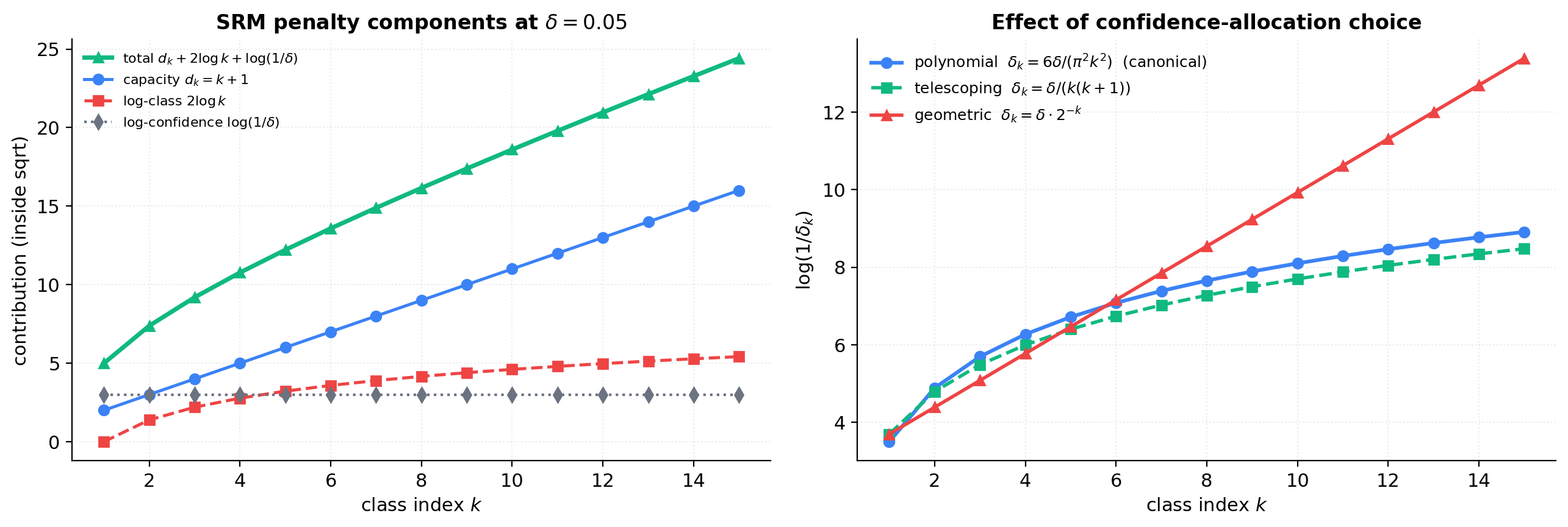
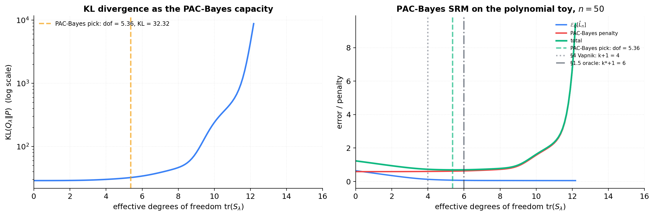
The figure below decomposes the SRM penalty into its three additive contributions on the polynomial-regression toy with $d_k = k+1$. At $\delta = 0.05$, $n = 50$, $k \in \{1, \ldots, 15\}$, the capacity term $d_k$ is linear and reaches 16 at $k = 15$; the log-class term $2 \log k$ is logarithmic and reaches $\approx 5.4$ at $k = 15$ (about a third of the capacity term); the log-confidence term $\log(1/\delta) \approx 3$ is constant. Capacity dominates the penalty; the $\log k$ price for considering an infinite family is real but small in practice.

The second panel compares three confidence-allocation choices for $\delta_k$. The canonical polynomial decay $\delta_k = 6\delta/(\pi^2 k^2)$ gives $\log(1/\delta_k) \sim 2 \log k$. The telescoping choice $\delta_k = \delta/(k(k+1))$ gives essentially the same asymptotic shape. The geometric choice $\delta_k = \delta \cdot 2^{-k}$ gives $\log(1/\delta_k) \sim k \log 2$ — linear in $k$, dramatically harsher. This is the visualization of why the polynomial decay is canonical: it’s the slowest-growing $\log(1/\delta_k)$ subject to $\sum_k \delta_k \le \delta$.

Classical VC-bound SRM (Vapnik 1995/1998)

The Vapnik penalty

The SRM oracle inequality (Theorem 1) is loss-agnostic and capacity-agnostic — it works for any per-class uniform convergence bound $(\dagger)$ we can produce. The Fundamental Theorem of Statistical Learning (PAC Learning, agnostic-PAC two-sided form) gives one for any class of finite VC dimension. For a class $\mathcal{H}$ with VC dimension $d$, any distribution $D$, and any $\delta \in (0, 1)$, with probability at least $1 - \delta$ over $S \sim D^n$,

$$\sup_{h \in \mathcal{H}} \bigl|L_D(h) - \hat L_S(h)\bigr| \;\le\; C \sqrt{\frac{d \log(2en/d) + \log(4/\delta)}{n}}, \tag{4.1}$$

where $C$ is a universal constant (the value depends on the loss function and the route taken through the FTSL proof — Sauer–Shelah + Hoeffding gives one constant, chaining bounds give a smaller one; the qualitative shape is what matters here). Plug in the canonical confidence allocation $\delta_k = 6\delta/(\pi^2 k^2)$ from §3.

Each term in the numerator has a meaning. $d_k \log(2n / d_k)$ is the capacity contribution — it comes from the Sauer–Shelah count of dichotomies a VC-$d_k$ class can produce on $n$ points and is the dominant term for moderate $k$ and $n$. $2 \log k$ is the union-bound cost from the confidence allocation $\delta_k = 6\delta/(\pi^2 k^2)$, the “price for considering infinitely many classes.” $\log(\pi^2/(6\delta))$ is the confidence-level cost. All inside a $\sqrt{1/n}$ envelope — the classical “slow rate” of statistical learning.

For regression with squared loss the same shape holds provided predictions and labels are bounded (truncate to $[-B, B]$ and the penalty picks up a multiplicative factor of $B^2$). The polynomial-regression toy from §1 satisfies $|m(x)| \le 1$ and $|\varepsilon| \le 1$ with overwhelming probability, so the truncation is invisible. For the polynomial family, the VC dimension of the threshold-classification variant equals the parameter dimension $d_k = k + 1$ — same shape for the regression effective DoF.

Derivation from FTSL

The derivation is the union-bound argument from §3 with $\varepsilon_k$ instantiated by (4.1). For each $\mathcal{H}_k$ at confidence level $\delta_k$,

$$\Pr\!\left[\sup_{h \in \mathcal{H}_k} \bigl|L(h) - \hat L_n(h)\bigr| > C \sqrt{\frac{d_k \log(2en/d_k) + \log(4/\delta_k)}{n}}\right] \;\le\; \delta_k.$$

Substituting $\delta_k = 6\delta/(\pi^2 k^2)$,

$$\log(4/\delta_k) \;=\; \log 4 + \log\!\frac{\pi^2 k^2}{6\delta} \;=\; 2\log k + \log\!\frac{4 \pi^2}{6\delta} \;=\; 2\log k + \log\!\frac{\pi^2}{6\delta} + \log 4.$$

The additive $\log 4$ rolls into the universal constant $C$ when we resolve the $\log$s into the form of Definition 3. The result is $(\dagger)$ with $\varepsilon_k(\delta_k, n) = \mathrm{pen}_V(\mathcal{H}_k, n, \delta)$. Applying Theorem 1 then gives the Vapnik SRM oracle inequality: with probability $\ge 1 - \delta$,

$$L(\hat h_{\hat k}) \;\le\; \inf_{k \ge 1} \bigl\{L^*(\mathcal{H}_k) \,+\, 2 \, \mathrm{pen}_V(\mathcal{H}_k, n, \delta)\bigr\}.$$

This is the original SRM bound from Vapnik (1995, 1998) — the form that motivated the entire framework.

SRM consistency

The oracle inequality is a finite-sample guarantee: for the given $n$ and $\delta$, the SRM estimator’s risk is no worse than the best in-family choice plus twice that class’s penalty. We’d also like an asymptotic guarantee — that as $n \to \infty$, the SRM estimator’s risk approaches the Bayes-optimal risk $L^* = \inf_h L(h)$, taken over all measurable $h$.

Two consequences. Convergence rate: if condition (a) is strengthened to a quantitative approximation rate — $L^*(\mathcal{H}_k) - L^* = O(k^{-\alpha})$ for some $\alpha > 0$ — then the convergence in Theorem 2 happens at a quantifiable rate, determined by trading $k$ off against the penalty (Lugosi and Zeger 1995). No rate without smoothness: without quantitative approximation conditions, the convergence in Theorem 2 can be arbitrarily slow (Devroye, Györfi, and Lugosi 1996, §7).

Proof of consistency

The argument is: pick a reference class $K$ that’s good enough in approximation, observe that its penalty vanishes as $n \to \infty$, plug both into the oracle inequality, take the limit.

Two structural notes about the proof. The reference $K$ is data-independent. This is essential: we pick $K$ based on the approximation property (a), apply the oracle inequality with $K$ on the right, and absorb the gap into the penalty. Trying to take $K = \hat k_n$ would defeat the argument, since the right-hand side of the oracle inequality is fixed before the data is seen. The proof says nothing about $\hat k_n$ itself. We never claim $\hat k_n \to \infty$ or $\hat k_n \to K^*$ for some optimal $K^*$ — what’s controlled is the risk, not the index. $\hat k_n$ can oscillate arbitrarily as long as the corresponding risk converges.

Vapnik SRM on the polynomial toy

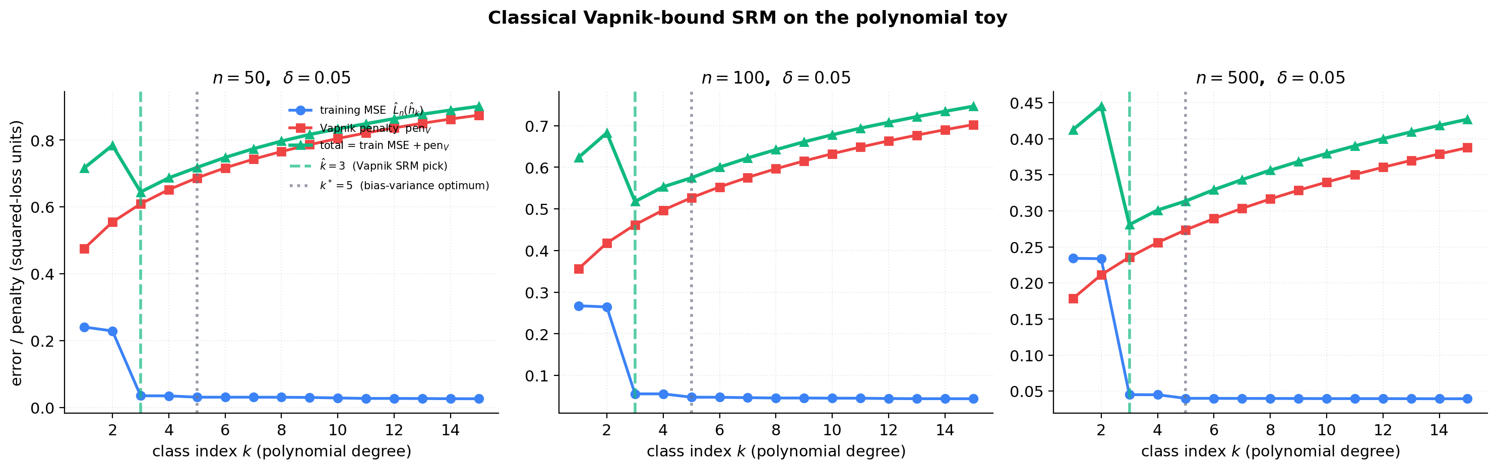
The figure below plots training MSE, the Vapnik penalty, and their sum as functions of $k$ on the polynomial-regression toy, at $n \in \{50, 100, 500\}$. The picked $\hat k$ is the argmin of the total; we also compute the bias-variance optimum $k^*$ from a small Monte Carlo for comparison.

The reader should see two things. The U-shape exists. Training MSE decreases monotonically, penalty grows monotonically, the sum has an interior minimum. The SRM rule is well-defined and computable from the sample alone. Vapnik SRM is conservative. The picked $\hat k$ is consistently smaller than the bias-variance optimum $k^*$ computed from §1’s MC. The Vapnik bound is the worst-case uniform-convergence rate over all distributions; on a benign distribution like ours, the actual generalization gap is much smaller than the bound, and the rule pays for the safety margin by under-fitting.

This sets up §5 directly. The Bartlett–Mendelson Rademacher SRM uses a data-dependent capacity measure (empirical Rademacher complexity on the actual sample) instead of the distribution-free VC dimension. On distributions where the worst case is not the worst case (which is most distributions), the Rademacher bound is tighter, and the picked $\hat k$ moves closer to $k^*$ — though at very small $n$ a McDiarmid confidence term can dominate and flip the relative tightness (§5.5).

The pedagogical $C = 1$ above keeps the §4.5 demo’s U-shape interior so the picked $\hat k$ is interpretable. The literal FTSL constant from chaining bounds is roughly 2–8, depending on the proof route; practitioners typically don’t use the literal Vapnik bound — they use Rademacher (§5), AIC/BIC (§8), or CV (§10) instead.

n: 50δ: 0.05C (Vapnik constant): 1.00

show §3.5 three-term decomposition (capacity + 2 log k + log(π²/(6δ)))

Vapnik SRM picks k̂_V = 3 at (n = 50, δ = 0.05, C = 1.00). On this benign distribution k̂_V is consistently smaller than the oracle k* ≈ 5 — the bound pays for distribution-freeness.

Rademacher-complexity SRM (Bartlett–Mendelson 2002)

From worst-case to data-dependent

The Vapnik penalty is the worst case over all distributions on $\mathcal{X}$ — it bounds the generalization gap of $\mathcal{H}_k$ uniformly over every conceivable input distribution. For any distribution where $\mathcal{H}_k$ exhibits less complexity than its worst case — because the data is on a low-dimensional manifold, or because the realized inputs lie in a benign region, or just because the noise structure happens to be helpful — the Vapnik bound overestimates the generalization gap, and the SRM rule built on it under-fits (§4.5).

The Rademacher complexity is empirical — it’s defined on the realized sample $X_1, \ldots, X_n$ and measures how well functions in $\mathcal{H}_k$ can align with random sign noise on that specific sample. If the class can’t fit Rademacher noise well on this particular $X$ — and for benign distributions, it usually can’t, by a $\sqrt{\log(n/d)}$ factor — the resulting penalty is tighter and the SRM rule picks a less conservative $\hat k$.

The replacement is mechanical: keep everything from §3 and §4, just swap the per-class uniform convergence bound. The Bartlett–Mendelson (2002) bound (Generalization Bounds, which establishes the bound via McDiarmid’s inequality and a symmetrization argument) replaces (4.1).

The Bartlett–Mendelson SRM penalty

For a function class $\mathcal{F}$ defined on a sample $S = (Z_1, \ldots, Z_n)$, the empirical Rademacher complexity is

$$\hat{\mathfrak{R}}_S(\mathcal{F}) \;=\; \mathbb{E}_{\sigma}\!\left[\sup_{f \in \mathcal{F}} \frac{1}{n}\sum_{i=1}^n \sigma_i f(Z_i)\right],$$

where $\sigma = (\sigma_1, \ldots, \sigma_n)$ are i.i.d. Rademacher variables uniform on $\{\pm 1\}$ (also developed in PAC Learning and Generalization Bounds). The Bartlett–Mendelson generalization bound: for the loss class $\mathcal{F}_k = \{(x, y) \mapsto \ell(h(x), y) : h \in \mathcal{H}_k\}$, with probability at least $1 - \delta$ over $S \sim D^n$,

$$\sup_{h \in \mathcal{H}_k} \bigl(L(h) - \hat L_n(h)\bigr) \;\le\; 2\hat{\mathfrak{R}}_S(\mathcal{F}_k) + 3 \sqrt{\frac{\log(2/\delta)}{2n}}. \tag{5.1}$$

The factor of 2 in front of $\hat{\mathfrak{R}}_S(\mathcal{F}_k)$ comes from the symmetrization step (passing from the data-sample $S$ to an i.i.d. ghost sample $S'$ and bounding by $2\mathfrak{R}_n$ — see Generalization Bounds). The $3\sqrt{\log(2/\delta)/(2n)}$ comes from two applications of McDiarmid’s bounded-differences inequality.

Plug $\delta_k = 6\delta/(\pi^2 k^2)$ into (5.1).

Three observations. The penalty is sample-dependent. The capacity term $\hat{\mathfrak{R}}_S(\mathcal{F}_k)$ has no $\log(n/d)$ factor: for nice classes its scaling is $\sqrt{d/n}$, not $\sqrt{d \log(n/d) / n}$ as in Vapnik. That $\sqrt{\log(n/d)}$ factor is the savings on benign distributions. For Lipschitz losses, Talagrand’s contraction lemma (Generalization Bounds) gives $\hat{\mathfrak{R}}_S(\mathcal{F}_k) \le L \cdot \hat{\mathfrak{R}}_S(\mathcal{H}_k)$, so we can compute Rademacher complexity on the hypothesis class and absorb $L$ into a constant.

The Rademacher SRM oracle inequality

Same shape as the Vapnik oracle inequality (§4), with $\mathrm{pen}_V$ replaced by $\mathrm{pen}_R$. The only thing that has changed is which uniform-convergence bound feeds into Theorem 1.

The bound is data-dependent in a sharper sense than Vapnik’s. The Vapnik bound depends on the sample only through $n$; the Rademacher bound depends on the sample through $\hat{\mathfrak{R}}_S$. Two practical consequences. Adaptivity: on benign samples, $\hat{\mathfrak{R}}_S(\mathcal{F}_k)$ is small even when $d_k$ is large. Sample-by-sample variability: the picked $\hat k$ can differ across samples even when the underlying distribution is the same — a feature, not a bug.

Proof

The proof is short because all the work is delegated. The McDiarmid + symmetrization machinery that establishes (5.1) lives in Generalization Bounds; the union-bound algebra lives in §3.4. What §5 contributes is the instantiation.

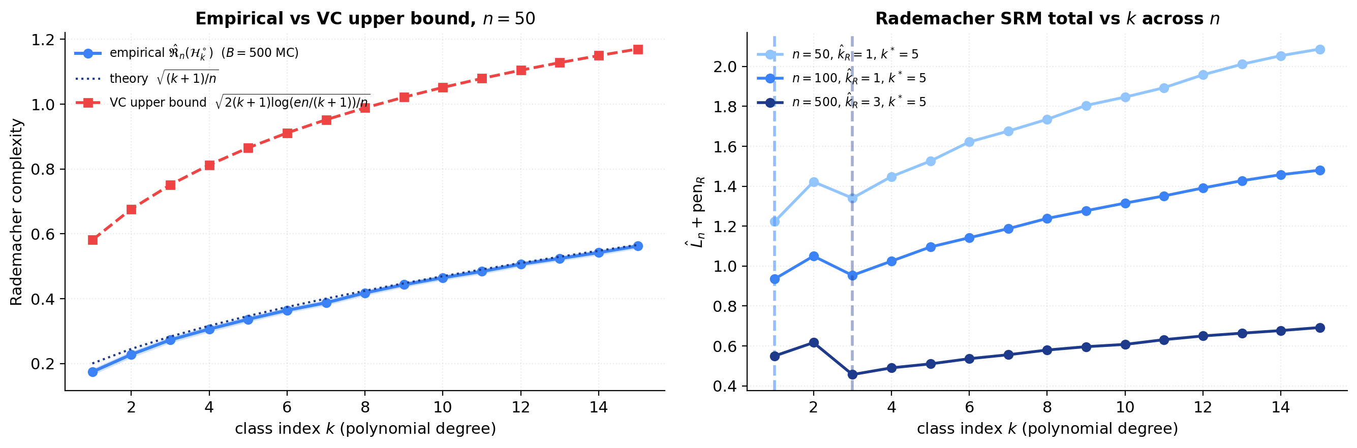
Empirical Rademacher vs the VC upper bound

The polynomial-regression toy admits a clean closed form for the empirical Rademacher complexity of the $L^2(P_n)$-unit-ball polynomial class $\mathcal{H}_k^\circ = \{h \in \mathcal{H}_k : \|h\|_n \le 1\}$. A direct computation (Cauchy–Schwarz in the $V^\top V$ inner product, where $V$ is the Vandermonde of the realized sample) gives

$$\sup_{h \in \mathcal{H}_k^\circ} \frac{1}{n}\sum_{i=1}^n \sigma_i h(X_i) \;=\; \frac{1}{\sqrt{n}} \|P_V \sigma\|,$$

where $P_V$ is the orthogonal projection onto the column space of $V$. So $\hat{\mathfrak{R}}_n(\mathcal{H}_k^\circ) = \mathbb{E}_\sigma[\|P_V \sigma\| / \sqrt{n}]$, estimated by Monte Carlo over $B = 500$ Rademacher draws. The closed form makes the computation deterministic — no actual fitting required, just orthogonal projection.

For comparison, the VC-implied upper bound (Massart’s lemma + Sauer–Shelah) is $\sqrt{2(k+1)\log(en/(k+1))/n}$. The factor that distinguishes them is the $\sqrt{\log(en/(k+1))}$ — the log savings from data-dependent vs distribution-free analysis.

The expected behavior — Rademacher tighter than Vapnik on benign distributions — is asymptotic. At small $n$ the Bartlett–Mendelson confidence term $3 \sqrt{\log(2\pi^2 k^2/(6\delta))/(2n)}$ can dominate the data-dependent capacity savings, and the Rademacher-picked $\hat k_R$ can come out smaller than $\hat k_V$ rather than larger. On our polynomial toy, $\hat k_R = 1$ at $n = 50$ and $n = 100$, while $\hat k_V = 3$ across all three sample sizes; the cross-over happens around $n \ge 200$. The honest reading: Rademacher is tighter than Vapnik asymptotically, on benign distributions; at small $n$ the McDiarmid confidence term can dominate and produce a conservative pick. The picture sharpens visibly as $n$ grows.

n: 100B (Rademacher MC draws): 300

overlay VC upper bound (Massart's lemma + Sauer-Shelah)

Empirical Rademacher sits below the VC upper bound; the gap is the √log(n/d_k) data-dependent savings. The savings shrink at small n because the McDiarmid confidence term in Definition 4 dominates (Rademacher SRM picks $\hat k_R = 1$ at n = 50, 100; cross-over near n ≥ 200).

Penalized ERM and soft SRM

From hard nesting to soft penalty

Sections 3–5 derived SRM as a discrete rule. The discreteness is a notational artifact. Every practical model class can be smoothly interpolated by a continuous capacity functional $C: \mathcal{H} \to \mathbb{R}_{\ge 0}$, and the discrete family is recovered as the level sets $\mathcal{H}_r = \{h \in \mathcal{H}_\infty : C(h) \le r\}$ of the capacity functional.

With a continuous capacity functional in hand, two natural problems present themselves. The constrained form:

$$\min_{h \in \mathcal{H}_\infty} \hat L_n(h) \quad \text{subject to} \quad C(h) \le r. \tag{6.1}$$

The penalized form replaces the constraint with a Lagrange multiplier:

$$\min_{h \in \mathcal{H}_\infty} \bigl\{\hat L_n(h) + \lambda C(h)\bigr\}, \qquad \lambda \ge 0. \tag{6.2}$$

Under mild convexity assumptions on $\hat L_n$ and $C$ — both satisfied for squared loss plus a convex norm penalty — strong Lagrangian duality holds: every solution of (6.1) at level $r$ is a solution of (6.2) at some $\lambda = \lambda(r)$, and vice versa (Boyd and Vandenberghe 2004, §5.5).

For SRM the practical consequence is that we don’t need to enumerate the discrete family. We can solve (6.2) for a continuous grid of $\lambda$ values, trace out the entire regularization path of solutions $\hat h_\lambda$, and pick $\hat\lambda$ to minimize a soft SRM objective — training error plus a penalty that depends on the effective capacity at $\lambda$.

The penalty parameter as a continuous SRM level

Let $\hat h_\lambda$ denote the solution of (6.2) at penalty parameter $\lambda$. As $\lambda$ varies from $0$ to $\infty$, $C(\hat h_\lambda)$ varies monotonically: $\lambda_1 < \lambda_2$ implies $C(\hat h_{\lambda_1}) \ge C(\hat h_{\lambda_2})$ (Tikhonov 1963).

So $\lambda$ acts as a continuous capacity dial. Small $\lambda$ = high capacity, large $\lambda$ = low capacity. This monotonicity is the soft analog of the nested-family inclusion: as $\lambda$ shrinks, the effective class $\mathcal{H}_{r(\lambda)} = \{h : C(h) \le r(\lambda)\}$ grows.

A useful capacity measure for the penalized-ERM regime is the effective degrees of freedom: $\mathrm{tr}(S_\lambda)$ for linear smoothers. For ridge regression with Vandermonde features $V$ and penalty $\lambda \|\alpha\|_2^2$,

$$S_\lambda = V (V^\top V + \lambda I)^{-1} V^\top, \qquad \mathrm{tr}(S_\lambda) = \sum_{j=1}^{k+1} \frac{s_j^2}{s_j^2 + \lambda},$$

where $s_j$ are the singular values of $V$. This trace decreases smoothly from $\mathrm{rank}(V) = k+1$ at $\lambda = 0$ to $0$ at $\lambda = \infty$, providing exactly the continuous interpolation we want.

The soft SRM estimator and its relationship to $\hat k$

The natural form replaces the discrete capacity term $d_k$ with effective DoF. The hard/soft correspondence: for each $\lambda$, Lagrangian duality identifies a unique $r(\lambda)$ such that $\hat h_\lambda$ solves the constrained problem at level $r(\lambda)$. For benign penalty constants, the picked effective DoF at $\hat\lambda$ should be close to the discrete SRM’s $\hat k + 1$.

Implicit nested families

Given any penalty functional $C$ and any $\lambda > 0$, the level set $\mathcal{H}_{r(\lambda)} = \{h : C(h) \le r(\lambda)\}$ is a well-defined hypothesis class, and as $\lambda$ varies these classes are nested. This is the implicit nested family generated by the penalty.

The consequence: any penalty-based method automatically inherits the SRM framework. The penalty type — $\ell_2$ for ridge, $\ell_1$ for lasso, Sobolev norm for spline smoothing, $\ell_0$-pseudo-norm for best-subset selection — determines the geometry of the implicit family, but the soft-SRM rule and its oracle inequality apply regardless.

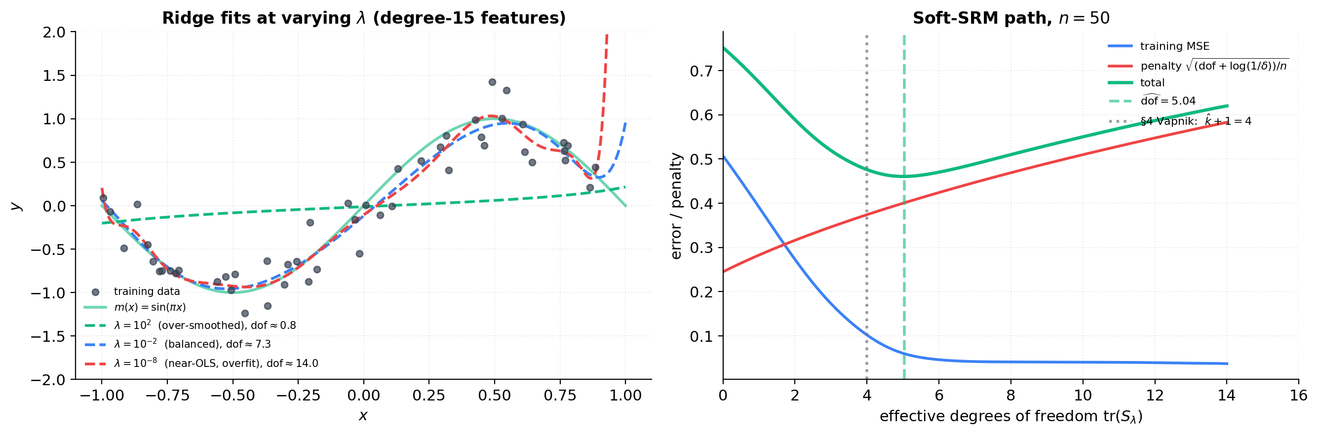
Soft-SRM path on the polynomial toy

The figure below uses the degree-15 Vandermonde feature matrix as the ambient parameter space and fits ridge regression $\min_\alpha \|Y - V\alpha\|_2^2 + \lambda \|\alpha\|_2^2$ for a logarithmic grid of $\lambda \in [10^{-8}, 10^6]$. For each $\lambda$ we compute training MSE, effective DoF $\mathrm{tr}(S_\lambda)$, and a simplified soft-SRM penalty $\sqrt{(\mathrm{tr}(S_\lambda) + \log(1/\delta))/n}$.

log₁₀ λ: -2.00 (λ = 1.00e-2)

Soft-SRM ridge: λ acts as a continuous capacity dial. Small λ = high capacity (overfit visible on the left); large λ = low capacity (underfit). The soft-SRM total picks λ̂ at the interior minimum, with picked effective DoF = 5.59.

SRM as regularization

Tikhonov regularization as soft SRM

Tikhonov (1963) introduced the regularization functional $\min_\theta \{\|Y - X\theta\|_2^2 + \lambda \|L\theta\|_2^2\}$ for some operator $L$. With $L = I$ this is standard ridge regression. With $L$ a discrete-derivative operator it becomes spline smoothing. With $L = D$ a finite-difference matrix it becomes total-variation denoising.

For SRM, the relevant fact is that Tikhonov with $L = I$ is precisely soft SRM (Definition 5) with capacity functional $C(\theta) = \|\theta\|_2^2$. The implicit nested family is the parameter-space ball $\mathcal{H}_r = \{\theta : \|\theta\|_2^2 \le r\}$. Geometrically the $\ell_2$ ball is rotationally symmetric — solutions shrink isotropically toward zero. No coefficient is ever set to exactly zero.

Ridge effective degrees of freedom

The effective DoF $\mathrm{tr}(S_\lambda)$ from §6 plays a dual role for ridge regression. First, it’s the capacity of the implicit family at $\lambda$. Second, it’s the Stein’s unbiased risk estimator (SURE) bias-correction term: the expected training MSE is biased downward from the population risk by $2 \sigma^2 \mathrm{tr}(S_\lambda)/n$.

For ridge on polynomial-Vandermonde features, the SVD gives $\mathrm{tr}(S_\lambda) = \sum_j s_j^2/(s_j^2 + \lambda)$ — a smooth monotone function from $k+1$ (OLS) to $0$. The SURE interpretation also gives a sample-only way to estimate $\hat\lambda$: minimize $\hat L_n(\hat h_\lambda) + 2 \hat\sigma^2 \mathrm{tr}(S_\lambda)/n$. This is Mallows’s $C_p$ in disguise (§8).

Lasso and the $\ell_1$ ball

Lasso (Tibshirani 1996) replaces Tikhonov’s $\ell_2$ penalty with $\ell_1$:

$$\hat\theta_\lambda^{\mathrm{Lasso}} \;\in\; \arg\min_\theta \bigl\{\|Y - X\theta\|_2^2 + \lambda \|\theta\|_1\bigr\}.$$

The implicit nested family is the $\ell_1$ ball $\mathcal{H}_r = \{\theta : \|\theta\|_1 \le r\}$ — a cross-polytope. The geometry forces solutions to lie on low-dimensional faces with most coordinates exactly zero. The natural capacity measure for lasso is sparsity — the number of nonzero coefficients. Zou, Hastie, and Tibshirani (2007) prove that this count equals the effective DoF in the SURE sense:

$$\mathrm{eff\_dof}(\hat\theta_\lambda^{\mathrm{Lasso}}) \;=\; \|\hat\theta_\lambda^{\mathrm{Lasso}}\|_0.$$

The Bickel-Ritov-Tsybakov (2009) lasso oracle inequality has exactly the SRM shape: $\|X(\hat\theta_\lambda^{\mathrm{Lasso}} - \theta^*)\|_n^2 \le c \cdot s^* \log p / n$, with $s^* = \|\theta^*\|_0$ the true sparsity — the capacity term $s \log p$ plays the role of $d_k \log(n/d_k)$ from §4.

In linear models, weight decay — adding $\lambda \|\theta\|_2^2$ to the loss — is literally Tikhonov regularization with $L = I$, hence soft SRM on the $\ell_2$ ball. The terminology comes from the gradient-descent update rule: $\theta_{t+1} = (1 - \eta\lambda)\theta_t - \eta\nabla\hat L_n(\theta_t)$. In deep networks the connection to classical SRM is murkier (§12), but the soft-SRM intuition still motivates the practice. For our polynomial-regression toy, weight decay is just ridge regression and the ridge effective-DoF analysis applies verbatim.

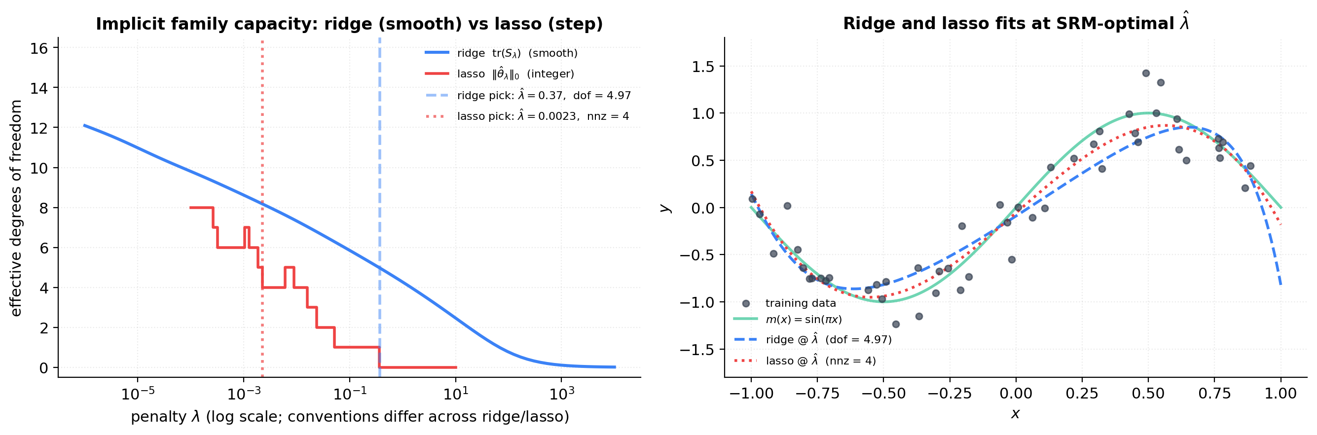
Ridge vs lasso on the polynomial toy

Fit ridge and lasso on the polynomial Vandermonde with the same training sample. Compute training MSE, effective DoF (smooth $\mathrm{tr}(S_\lambda)$ for ridge, integer-valued $\|\hat\theta\|_0$ for lasso), and the soft-SRM total. The figure compares ridge $\hat\lambda$ + effective DoF, lasso $\hat\lambda$ + number of nonzeros, §4 Vapnik hard-SRM $\hat k + 1$, and the §1 bias-variance oracle $k^* + 1$. All four should fall in a narrow band on this benign toy.

Ridge log₁₀ λ: -2.00 (λ = 1.0e-2)Lasso log₁₀ λ: -2.00 (λ = 1.0e-2)

Ridge and lasso are both soft SRM on different implicit families. Ridge ℓ² ball: rotationally symmetric, smooth effective DoF. Lasso ℓ¹ ball: cross-polytope, integer-valued capacity. The user picks the penalty geometry; SRM picks the level.

SRM and information criteria

AIC

The Akaike Information Criterion (Akaike 1973) is $\mathrm{AIC}_k = -2 \log p(Y \mid \hat\theta_k) + 2 d_k$. For Gaussian-noise regression with plug-in $\sigma^2$, AIC is equivalent to picking $\hat k$ minimizing $\hat L_n(\hat h_k) + 2 \sigma^2 d_k / n$. So AIC is exactly the SRM rule with capacity penalty $\mathrm{pen}_{\mathrm{AIC}}(d_k, n) = 2\sigma^2 d_k / n$ — linear in $d_k$, no $\log$ factor, no confidence parameter.

Motivation: Akaike derived AIC by asking, asymptotically, which model gives the smallest Kullback–Leibler divergence from the true distribution. The rule is calibrated for prediction risk, not selection consistency: AIC is asymptotically efficient for prediction.

BIC

The Bayesian Information Criterion (Schwarz 1978) is $\mathrm{BIC}_k = -2 \log p(Y \mid \hat\theta_k) + d_k \log n$ — penalty $d_k \log n$ rather than $2 d_k$. For Gaussian-noise regression, BIC penalty is $\sigma^2 d_k \log n / n$. For $n \ge e^2 \approx 7.4$, $\log n > 2$, so BIC is strictly more conservative than AIC.

Motivation: Schwarz derived BIC as a Laplace approximation to the negative log marginal likelihood of a Bayesian model with a flat prior. BIC is consistent for selection: if the true model lies in the family, BIC picks it with probability $\to 1$ as $n \to \infty$. The AIC vs BIC distinction: AIC minimizes prediction risk asymptotically, BIC identifies the true model asymptotically.

MDL

The Minimum Description Length principle (Rissanen 1978) views model selection as data compression. The “best” coding scheme for parameters (Rissanen’s universal Bayesian code) yields $\mathrm{MDL}_k \approx -\log p(Y \mid \hat\theta_k) + (d_k/2) \log n + O(1)$. Doubling and comparing to BIC: $2 \mathrm{MDL}_k \approx \mathrm{BIC}_k$ asymptotically. MDL and BIC are the same rule from different starting points. See Minimum Description Length for the coding-theoretic substrate.

Unification

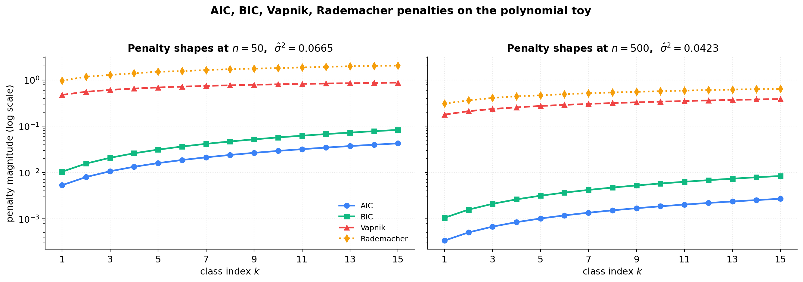
All five SRM rules fit the same template — pick $\hat k$ minimizing $\hat L_n(\hat h_k) + \mathrm{pen}(d_k, n, \delta)$. They differ in the penalty function:

Rule	Penalty	Shape
AIC	$2\sigma^2 d_k / n$	linear in $d_k$; no $\log n$; no $\delta$
BIC, MDL	$\sigma^2 d_k \log n / n$	linear in $d_k$; $\log n$; no $\delta$
Vapnik	$C \sqrt{(d_k \log(n/d_k) + \log(1/\delta)) / n}$	square-root in $d_k$; $\log n$; finite-sample $\delta$
Rademacher	$2 \hat{\mathfrak{R}}_n + 3 \sqrt{\log(1/\delta_k)/(2n)}$	empirical; data-dependent; finite-sample $\delta$

Three structural differences. Capacity shape: AIC/BIC are linear (parametric, fast rate); Vapnik/Rademacher are square-root (non-parametric, slow rate). $\log n$ factor: BIC and Vapnik have it; AIC and Rademacher don’t. Confidence parameter: Vapnik and Rademacher are finite-sample bounds; AIC and BIC are asymptotic.

Each targets a different goal: AIC for asymptotic prediction efficiency; BIC/MDL for selection consistency; Vapnik for worst-case finite-sample generalization; Rademacher for data-dependent finite-sample generalization.

Penalty shapes and pick-agreement

For $n \in \{50, 100, 500\}$ on the polynomial toy, compute training MSE and each of the four penalties as functions of $k$. The figure plots the four penalty shapes on a log y-scale (the bound-based and asymptotic penalties span ~50× in magnitude) and tabulates the picked $\hat k$ for each rule.

n: 50σ (noise std): 0.20

AIC pick: 5

BIC pick: 3

Vapnik pick: 3

Rademacher pick: 1

Same SRM template, different calibrations, different picks. AIC/BIC are parametric/linear; Vapnik/Rademacher are non-parametric/square-root and dominate AIC/BIC by 1-2 orders of magnitude.

SRM and PAC-Bayes

From class-indexed nesting to posterior-averaged capacity

PAC-Bayes generalizes SRM substantially: the rule produces a probability distribution $Q$ over hypotheses, with the predictor being either the posterior-mean function $\bar h_Q(x) = \mathbb{E}_{h \sim Q}[h(x)]$ or a stochastic sample from $Q$.

The setup. Fix a prior $P$ over $\mathcal{H}$ chosen before seeing the data. After observing $S$, choose a posterior $Q$ — any data-dependent distribution, subject to $Q \ll P$. The PAC-Bayes framework bounds the posterior-averaged generalization error $\mathbb{E}_{h \sim Q}[L(h)]$ in terms of posterior-averaged training error and KL divergence $\mathrm{KL}(Q \| P)$. The implicit nested family is indexed by KL: $\mathcal{Q}_r = \{Q : \mathrm{KL}(Q \| P) \le r\}$. PAC-Bayes is smooth SRM with KL as the capacity functional.

The PAC-Bayes bound (Catoni–McAllester family)

The bound is uniform over all $Q$ by a continuous-$Q$ MGF argument (PAC-Bayes Bounds contains the full derivation via Donsker–Varadhan). Catoni’s tighter 2007 form replaces the square-root capacity term with an exponentially-tilted bound sharper for small $\mathbb{E}_Q[\hat L_n]$; for SRM purposes the qualitative shape is identical.

KL divergence as a continuous capacity measure

For Gaussian posteriors and priors, KL has a closed form. With $P = \mathcal{N}(0, \sigma_P^2 I_d)$ and $Q = \mathcal{N}(\mu_Q, \sigma_Q^2 I_d)$,

$$\mathrm{KL}(Q \| P) \;=\; \frac{1}{2}\left(\frac{d \sigma_Q^2 + \|\mu_Q\|^2}{\sigma_P^2} \,-\, d \,+\, d \log \frac{\sigma_P^2}{\sigma_Q^2}\right). \tag{9.2}$$

KL is monotone in $\|\mu_Q\|^2$ — the connection to Tikhonov regularization from §7 becomes explicit at the PAC-Bayes level. Minimizing $\mathbb{E}_Q[\hat L_n] + \sqrt{\mathrm{KL}/(2n)}$ over a Gaussian $Q$ centered at the ridge estimator produces a penalty $\propto \|\hat\alpha_\lambda\|^2 / \sigma_P^2$.

Soft-to-hard SRM limit

Posterior concentrates on a single hypothesis: $\mathrm{KL}(Q \| P) = \infty$ for any continuous prior $P$. To recover hard SRM, use a discrete prior: $P$ uniform over $\{\hat h_1, \ldots, \hat h_K\}$, $Q$ point-mass on one $\hat h_k$, $\mathrm{KL}(Q \| P) = \log K$ — the union-bound rule from §3 as a special case.

Posterior equals prior: $\mathrm{KL}(Q \| P) = 0$ gives a tight bound on the prior-mean predictor, which has no data-adaptation.

The PAC-Bayes-optimal posterior is the Gibbs posterior $Q^*(h) \propto P(h) \exp(-\beta \cdot \hat L_n(h))$ — the analog of the Bayesian posterior, with $\beta$ controlling concentration. The PAC-Bayes-optimal $\beta$ trades off the two extremes: exactly the SRM trade-off. See PAC-Bayes Bounds for the full Gibbs construction.

PAC-Bayes on the polynomial toy

The figure uses the polynomial Vandermonde features of degree 15 as the parameter space ($d = 16$). Prior $P = \mathcal{N}(0, \sigma_P^2 I_{16})$ with $\sigma_P = 1$. For a logarithmic grid of $\lambda$, the posterior mean is set to the ridge estimate and the posterior covariance to $\tau^2 I_{16}$ with $\tau = 0.1$. We compute KL via (9.2), posterior-averaged training error, and PAC-Bayes total.

The $\tau = 0.1$ choice is a pedagogical simplification — the proper Bayesian-ridge posterior covariance is $\sigma^2 (V^\top V + \lambda I)^{-1}$, which depends on $\lambda$. Decoupling $\tau$ from $\lambda$ keeps the §9 demo focused on the KL-as-capacity story without re-engineering for the full Bayesian-ridge posterior.

σ_P (prior width): 1.00τ (posterior width): 0.10

Picked effective DoF at λ̂: 5.67. KL is the continuous capacity measure; the prior σ_P chooses *which* implicit family, the posterior τ chooses *where* on the family to land.

Cross-validation as data-driven SRM

CV as a complexity-penalty surrogate

Cross-validation takes a different route from the bound-based rules: estimate the population risk by holding out part of the sample. The $K$-fold cross-validation procedure for $\mathcal{H}_k$ partitions $S$ into $K$ folds, fits $\hat h_k^{(-j)}$ on the other $K-1$ folds, and evaluates on the held-out fold:

$$\hat L^{\mathrm{CV}}_k \;=\; \frac{1}{K} \sum_{j=1}^K \frac{1}{|S^{(j)}|} \sum_{i \in S^{(j)}} \ell\bigl(\hat h_k^{(-j)}(X_i), Y_i\bigr).$$

CV picks $\hat k_{\mathrm{CV}} \in \arg\min_k \hat L^{\mathrm{CV}}_k$ and returns $\hat h_{\hat k_{\mathrm{CV}}}$ refit on the full sample. The key structural fact: no explicit penalty. $\hat L^{\mathrm{CV}}_k$ is an unbiased estimator of the population risk of the $(K-1)/K$-subsample fit. The trade-off is information loss: CV uses $1/K$ of the data for testing per fold, so it has higher statistical variance than bound-based rules.

A CV oracle inequality

The $\sqrt{\log M / n_{\mathrm{test}}}$ rate matches SRM up to constants. For infinite families, the analog (Bartlett, Lugosi, Mendelson 2002; Yang 2007) replaces $\log M$ with a stability-based or VC-based measure. Proof sketch: Hoeffding on each fold plus union bound over $M$ candidates.

The CV-variance vs SRM-stability trade-off

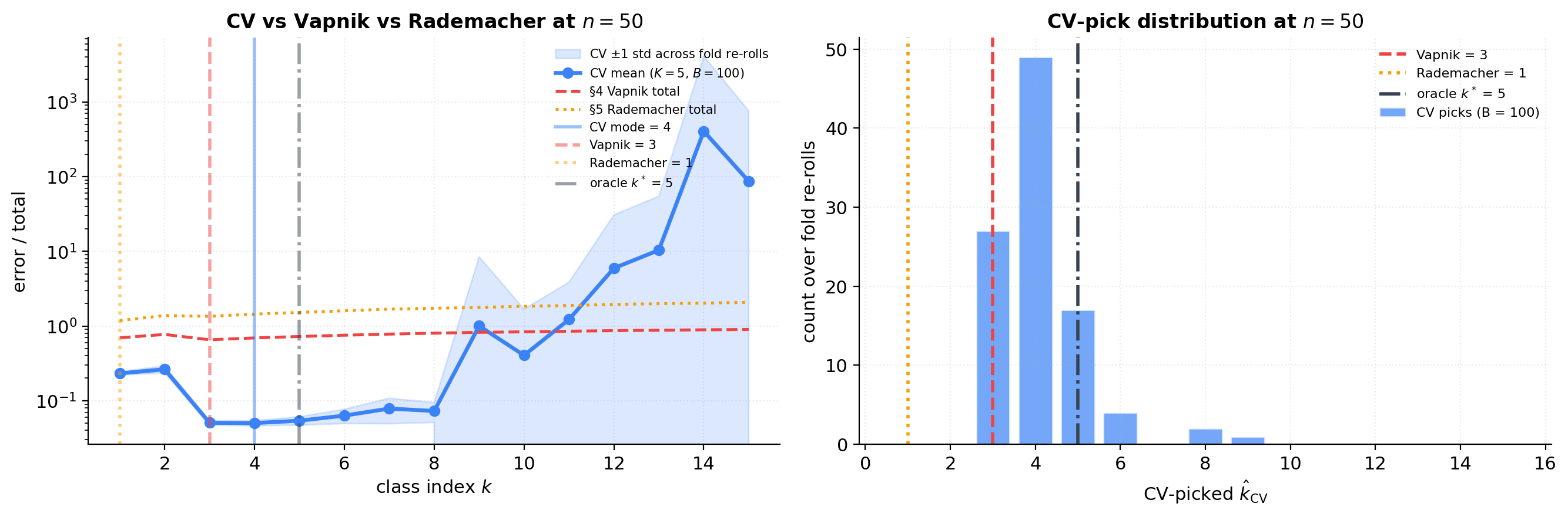
CV has higher statistical variance — the score depends on the random fold partition, with width 1–3 degrees on the polynomial toy across 100 partitions. Bound-based SRM depends on the algorithm’s stability — Vapnik is loose for stable algorithms, tight for unstable. Practical rule: CV for complex algorithms (deep nets, ensembles); bound-based SRM for simple families with clean capacity analysis.

When CV picks differently from SRM

Three regimes: loose bound constants (Vapnik’s $C$ slack); asymptotic vs finite-$n$ (AIC/BIC are asymptotic, CV is finite-sample); fold-partition noise (CV varies by 1–2 across rerolls). Agreement is reassuring; disagreement is diagnostic.

CV vs Vapnik vs Rademacher

Run 5-fold CV at $n = 50$ with 100 random fold partitions. The figure aggregates to the mean CV curve, $\pm 1$ std band across partitions, and the distribution of picked $\hat k$. The histogram of CV picks shows fold-to-fold variability concretely.

K (folds): 5B (rerolls): 50n: 50

CV pick mode: 3 across 50 fold rerolls at K=5, n=50. The histogram shows fold-partition variance directly — 1–3 degrees of spread is typical at small n.

Worked example: polynomial regression with SRM

Setup recap

The toy from §1, used throughout: $X \sim \mathrm{Uniform}(-1, 1)$, $m(x) = \sin(\pi x)$, $\varepsilon \sim \mathcal{N}(0, 0.2^2)$, $n \in \{50, 100, 500\}$, $\mathcal{H}_k =$ polynomials of degree $\le k$.

Bias-variance Monte Carlo

The bias-variance decomposition from §1, with $B = 200$ replicates per sample size. The argmin of MSE over $k$ defines the bias-variance oracle $k^*(n)$.

The agreement matrix

For each rule and each $n$, the picked $\hat k$ on the executed notebook (NumPy PCG64 seed 20260512):

Rule (this seed)	$n = 50$	$n = 100$	$n = 500$
AIC	5	5	5
BIC	5	5	5
Vapnik ($C = 1$)	3	3	3
Rademacher	1	1	3
5-fold CV (mode, 100 rerolls)	4	5	5
PAC-Bayes (degree $= \lfloor \mathrm{DoF}\rfloor - 1$)	4	5	6
Oracle $k^*$	5	5	5

Three patterns: the picks cluster within a 4-degree band; AIC and BIC pick largest, Vapnik smallest at moderate $n$; all picks shift upward (or hold steady) with $n$ (consistency in action). The one surprise is Rademacher at small $n$ — the McDiarmid confidence term in $\mathrm{pen}_R$ dominates the data-dependent capacity savings on this benign distribution, and the rule picks $\hat k_R = 1$ rather than the $\hat k_R \ge \hat k_V$ asymptotic prediction.

Sensitivity to noise, sample size, and confidence

Noise variance: larger $\sigma$ shifts oracle $k^*$ down. AIC and BIC have explicit $\sigma^2$ factors. Vapnik/Rademacher are $\sigma$-free but indirectly affected via the training-error curve. Sample size: all rules shift up with $n$. Confidence parameter: only Vapnik, Rademacher, PAC-Bayes depend on $\delta$; AIC, BIC, CV are $\delta$-free.

Agreement matrix, money shot, sensitivity sweep

n: 50σ: 0.20K (folds): 5δ: 0.05

headline rule:AICBICVapnikRademacherCVPAC-BayesOracle k*

Agreement matrix

Money shot + sensitivity bar

Every rule, every pick, at this (n, σ, K, δ). Set the headline-rule selector to swap whose fit drives the money shot. The agreement matrix reveals when rules disagree (small n) and when they cluster (large n).

SRM in practice: SVMs and beyond

SVMs and the $C$-parameter as SRM

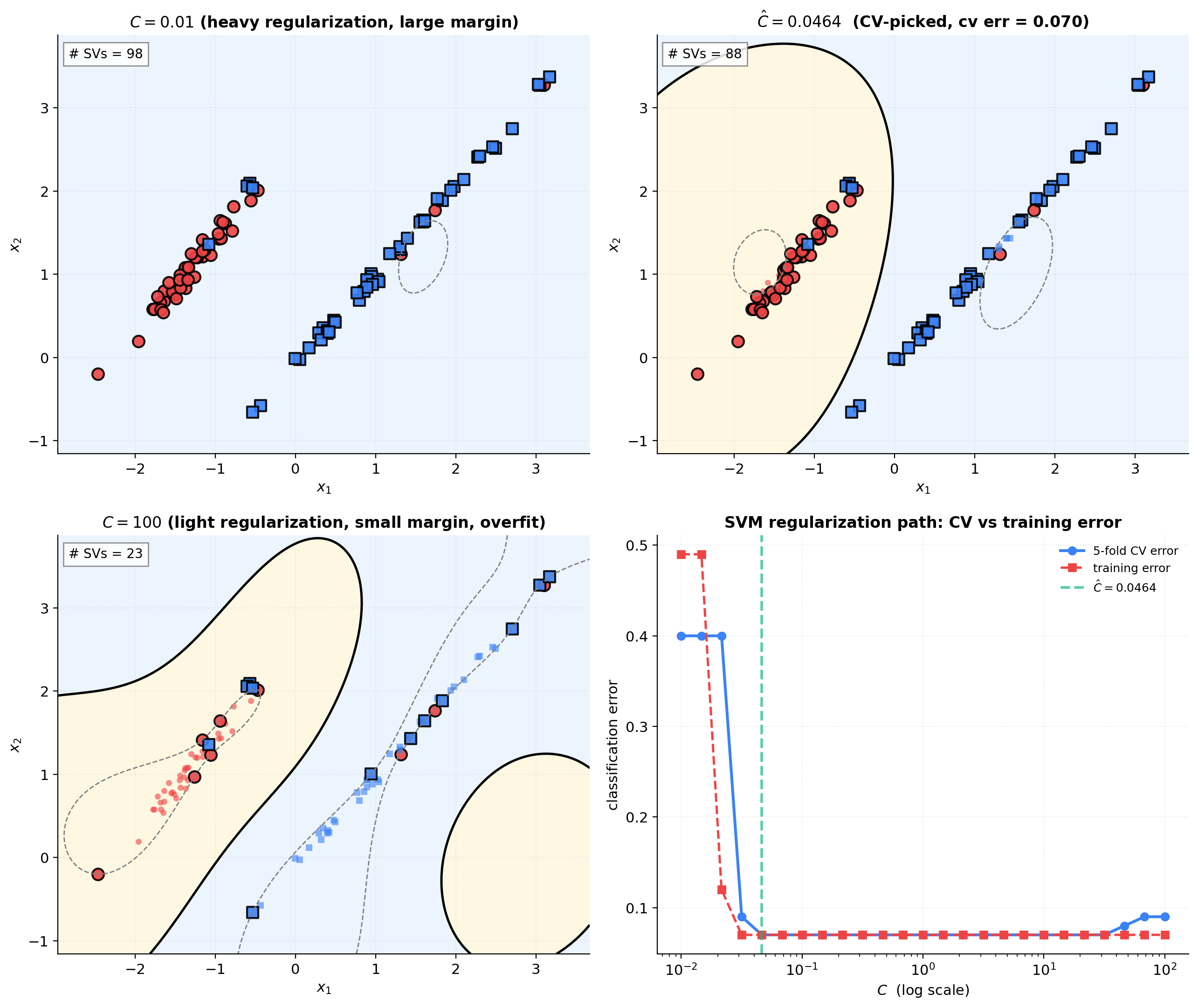
Soft-margin SVMs (Cortes and Vapnik 1995) are the canonical classical-SRM application:

$$\min_{w, b, \xi} \;\;\frac{1}{2}\|w\|_2^2 + C \sum_{i=1}^n \xi_i \quad \text{subject to} \quad y_i (\langle w, \phi(x_i) \rangle + b) \ge 1 - \xi_i, \;\xi_i \ge 0.$$

This is soft SRM (Definition 5) with hinge loss and capacity functional $C(w) = \tfrac{1}{2}\|w\|_2^2$. The implicit nested family is the margin-balls $\mathcal{H}_\gamma = \{(w, b) : \|w\|_2 \le 1/\gamma\}$. The capacity calculation is celebrated: for an RKHS with bounded kernel $K(x, x) \le R^2$,

$$\hat{\mathfrak{R}}_n(\mathcal{H}_\gamma) \;\le\; \frac{R}{\gamma \sqrt{n}}.$$

Dimension-free — this is why kernel methods work in infinite-dimensional spaces without curse-of-dimensionality penalty.

Neural networks: where classical SRM goes loose

For a depth-$L$ neural network with $W$ total parameters, $\dim_{\mathrm{VC}} = \Theta(W L \log W)$ (Bartlett, Maiorov, Meir 1998). For $W = 10^7$, $L = 50$, that’s $\approx 5 \times 10^9$ — vacuous bound. Why classical SRM fails: the bound is uniform over $\mathcal{H}_w$ but SGD explores only a small subset; implicit regularization biases SGD toward low-norm solutions. Active research: spectral norms (Bartlett, Foster, Telgarsky 2017), PAC-Bayes with data-dependent priors (Dziugaite and Roy 2017), sharpness (Foret et al. 2021).

The overparameterized regime

Modern ML operates with $W \gg n$. Classical SRM says generalization should be terrible; empirically it’s fine. Three theory threads address the puzzle: benign overfitting (Bartlett, Long, Lugosi, Tsigler 2020), implicit regularization, norm-based margin bounds. None is yet predictive. Practical model selection still uses CV.

Double descent as the modern complication

Belkin, Hsu, Ma, Mandal (2019); Nakkiran et al. (2020): test risk as a function of capacity has two regimes. Classical regime ($W \ll n$): U-curve. Interpolation threshold ($W \approx n$): catastrophic peak. Modern regime ($W \gg n$): second descent, often below the classical minimum. Detailed treatment: Double Descent (coming soon).

The double-descent picture: classical U-curve (bias → variance) up to the interpolation threshold W ≈ n, catastrophic peak at the threshold, then a second descent in the modern overparameterised regime (W ≫ n). Sketch only — full treatment in Double Descent (coming soon).

SVM-$C$ sweep on a 2D classification toy

A 2D binary classification toy ($n = 100$, two Gaussian clusters). RBF-kernel SVM across $C \in [10^{-2}, 10^2]$. 5-fold CV picks $\hat C$. The four-panel figure shows decision boundaries at three $C$ values plus the CV error vs $C$ path.

Connections and limits

Tightness of the bounds

The Vapnik bound is loose by orders of magnitude on benign distributions — the price of being distribution-free. Rademacher tightens by going data-dependent (factor of $\sqrt{\log(n/d_k)}$ for nice distributions). PAC-Bayes tightens further by leveraging the prior. Lower bounds: the Vapnik rate is tight up to constants for some problem instances — the worst case is real, just not the average case. Practitioner hierarchy: Vapnik for deterministic guarantee with looseness tolerance; Rademacher for tighter guarantee on the specific dataset; PAC-Bayes for prior knowledge; CV for empirical right-answer.

Non-nested families

Many families aren’t nested: $k$-NN, different SVM kernels, decision trees by leaf count, bagging. The §2.4 workaround: drop the strict inclusion requirement and keep only the capacity-indexed part. The union-bound argument (§3.1) never used $\mathcal{H}_j \subset \mathcal{H}_k$ — only $\sum_k \delta_k \le \delta$. The same SRM estimator and oracle inequality work for any countable capacity-indexed family. What’s lost is interpretive: the bias term doesn’t decompose monotonically. For unions of finite collections of nested chains (e.g., SVM with multiple kernels), hierarchical SRM with $\delta_m = \delta/M$ across chains works cleanly.

Computational cost

Bound-based SRM: per-class fit cost × number of classes. Cheap for polynomial regression; manageable for SVMs; dominated by training cost for deep nets. CV: $K \times$ per-class fit cost. Expensive for large neural nets. Implicit regularization (early stopping, dropout): essentially free but theoretically opaque. The trade-off: clean theory and low cost (bounds) vs universal applicability (CV) vs cheap-but-opaque (implicit).

What SRM doesn’t tell you

Distribution shift: SRM assumes i.i.d. training and test data. Real-world shift breaks this; domain adaptation is the active research area (Ben-David et al. 2010). Agnostic-PAC gap: SRM bounds $L(\hat h_{\hat k}) - L^*(\mathcal{H}_{\hat k})$, not $L(\hat h_{\hat k}) - L^*$ (Bayes-optimal gap); if the family doesn’t approximate Bayes-optimal well, SRM is vacuous on absolute risk. Model misspecification: classical SRM assumes well-specified models; under misspecification, “best-in-class” $L^*(\mathcal{H}_k)$ may be far from any meaningful target. Other: family choice (vs index within family), loss-function choice, adversarial robustness, active learning. SRM is precise for given fixed family + i.i.d. sampling, how to pick adaptively; silent on everything else.

Where to go next

• Double Descent (coming soon) — the modern overparameterized regime; benign overfitting; implicit regularization.
• PAC-Bayes Bounds — full PAC-Bayes theory; Donsker-Varadhan, Maurer’s lemma, Catoni.
• Generalization Bounds — McDiarmid plus symmetrization; Bartlett-Mendelson Rademacher bounds in detail.
• PAC Learning — foundational VC plus Sauer-Shelah plus FTSL plus Rademacher.
• Stacking and Predictive Ensembles — ensembling and Bayesian model averaging as soft model averaging across the SRM family.

Beyond formalML: Massart’s Concentration Inequalities and Model Selection (Springer 2007); Mohri, Rostamizadeh, Talwalkar’s Foundations of Machine Learning (MIT 2018); Vapnik’s Statistical Learning Theory (Wiley 1998).

Computational notes

Every numerical experiment in this topic runs in under a second per slider commit on a 2020-era CPU. The computational bottleneck across §§4–11 is the polynomial Vandermonde-based linear algebra; below is the Python skeleton used to produce the figures.

import numpy as np

def make_data(n, sigma, rng):
    """Polynomial-regression toy: X ~ U(-1,1), Y = sin(πX) + N(0, sigma²)."""
    X = rng.uniform(-1.0, 1.0, size=n)
    Y = np.sin(np.pi * X) + sigma * rng.standard_normal(n)
    return X, Y


def vapnik_penalty(d_k, n, k, delta, C=1.0):
    """Vapnik penalty (Definition 3) with universal constant C exposed."""
    capacity = d_k * np.log(2 * n / np.maximum(d_k, 1))
    klog = np.where(np.asarray(k) <= 1, 0.0, 2 * np.log(np.maximum(k, 1)))
    conf = np.log((np.pi ** 2) / (6 * delta))
    return C * np.sqrt((capacity + klog + conf) / n)


def empirical_rademacher_polynomial(X, k, B, rng):
    """Closed-form empirical Rademacher complexity for the polynomial unit ball."""
    V = np.vander(X, k + 1, increasing=True)
    Q, _ = np.linalg.qr(V)  # thin QR — orthonormal basis for col(V)
    n = len(X)
    norms = np.empty(B)
    for b in range(B):
        sigma = rng.choice([-1, 1], size=n)
        norms[b] = np.linalg.norm(Q.T @ sigma) / np.sqrt(n)
    return norms.mean(), norms.std() / np.sqrt(B)


def estimate_sigma2(X, Y, k_max):
    """Unbiased plug-in noise variance from SVD-pseudoinverse OLS at k_max."""
    V = np.vander(X, k_max + 1, increasing=True)
    coef, *_ = np.linalg.lstsq(V, Y, rcond=None)
    rss = float(np.sum((Y - V @ coef) ** 2))
    return rss / max(len(Y) - (k_max + 1), 1)


def aic_penalty(d_k, n, sigma2):
    return 2.0 * sigma2 * d_k / n


def bic_penalty(d_k, n, sigma2):
    return sigma2 * d_k * np.log(n) / n


def ridge_fit_predict(X, Y, k_max, lam):
    V = np.vander(X, k_max + 1, increasing=True)
    n, d = V.shape
    A = V.T @ V + lam * np.eye(d)
    alpha = np.linalg.solve(A, V.T @ Y)
    return V @ alpha, alpha


def ridge_effective_dof(X, k_max, lam):
    V = np.vander(X, k_max + 1, increasing=True)
    s = np.linalg.svd(V, compute_uv=False)
    return float(np.sum(s ** 2 / (s ** 2 + lam)))

Numerical pitfalls worth flagging. Vandermonde conditioning at high degree: the monomial Vandermonde on $n = 50$ points at degree 15 has condition number $\approx 10^{20}$; use SVD-pseudoinverse (numpy.linalg.lstsq with rcond=None) or QR rather than the normal equations directly. Numerical lasso convergence: at very small $\lambda$, the lasso fit on a degree-15 Vandermonde converges slowly under coordinate descent; set max_iter generously and suppress benign convergence warnings, or use the Chebyshev basis as the working basis. Plug-in $\hat\sigma^2$: at small $n$ relative to $d_{\max}$ the unbiased estimator $\mathrm{RSS}/(n - d_{\max})$ has non-trivial variance, and BIC picks can shift by 1–2 degrees across reseeds. The agreement matrix above gives the central pick at the notebook seed; expect drift across alternative seeds.