VC Dimension

Motivation: why finite-class arguments break for infinite hypothesis classes

The PAC Learning topic developed the sharpest tool we have for finite hypothesis classes: take Hoeffding’s inequality on a single hypothesis, apply the union bound over all $|\mathcal{H}|$ of them, and a sample size of $n = O((\log |\mathcal{H}| + \log(1/\delta))/\epsilon^2)$ suffices for uniform convergence at level $\epsilon$ with confidence $1-\delta$. The bound is tight in $|\mathcal{H}|$, transparent in its derivation, and useless the moment we try to use it on anything we’d want to learn — every real-parameter class has $|\mathcal{H}| = \infty$, and $\log \infty$ shuts the argument down. The question for this whole topic: what’s the right combinatorial object to put in place of $|\mathcal{H}|$ when the cardinality counts the wrong thing?

The finite-class union-bound recap

Fix the standard setup. We have a labeled sample $S = ((X_1, Y_1), \dots, (X_n, Y_n))$ drawn i.i.d. from a distribution $D$ on $\mathcal{X} \times \{0, 1\}$, a binary hypothesis class $\mathcal{H} \subseteq \{0, 1\}^{\mathcal{X}}$, the population risk $R(h) = \Pr_D[h(X) \ne Y]$, and the empirical risk $\hat R(h) = \frac{1}{n}\sum_{i=1}^n \mathbb{1}[h(X_i) \ne Y_i]$. Hoeffding’s inequality applied to the $n$ Bernoulli indicators gives $\Pr(|R(h) - \hat R(h)| > \epsilon) \le 2 \exp(-2 n \epsilon^2)$. The PAC framework wants this uniformly over the whole class, so we union-bound across $\mathcal{H}$:

$$\Pr\!\bigl(\exists h \in \mathcal{H} : |R(h) - \hat R(h)| > \epsilon\bigr) \le 2 |\mathcal{H}| \exp(-2 n \epsilon^2).$$

Setting the right-hand side to $\delta$ and solving for $n$ gives the canonical finite-class sample-complexity bound

$$n \ge \frac{\log|\mathcal{H}| + \log(2/\delta)}{2 \epsilon^2}, \quad\quad (1.1)$$

the headline result of PAC Learning §3. The logarithm is the union bound’s signature: every extra hypothesis costs us $\log$ in the sample size. The bound stays usable for surprisingly large finite classes — billions of hypotheses cost twenty-something samples — but it requires $|\mathcal{H}| < \infty$.

What |H| should “really” mean

Take the simplest infinite class: half-lines on the real line, $\mathcal{H}_{\text{half-line}} = \{h_a : a \in \mathbb{R}\}$ with $h_a(x) = \mathbb{1}[x \ge a]$. There are uncountably many hypotheses and bound (1.1) instantly degenerates: $\log|\mathcal{H}_{\text{half-line}}| = \infty$ forces $n = \infty$. Yet half-lines are intuitively a small class — one real degree of freedom, a handful of points should suffice. The bound is counting something it shouldn’t be counting.

The issue is that the union bound treats every $h_a$ as a fresh draw from concentration’s perspective, but on any fixed sample $S$ most of those thresholds are behaviorally indistinguishable. Two thresholds $a, a'$ in the same gap between consecutive sample points produce the same labels on $S$. The hypotheses are different as functions on $\mathbb{R}$, but identical as labelings of $S$. If $\mathcal{H}_{\text{half-line}}$ has uncountably many functions but only $n + 1$ distinct labelings of any $n$-point sample, the right effective cardinality for the union bound is $n + 1$, not $\infty$.

The right object: labelings on a fixed sample, not functions on the input space

For a sample $S = (x_1, \dots, x_n)$ and a class $\mathcal{H}$, the restriction of $\mathcal{H}$ to $S$ is

$$\mathcal{H}_{|S} = \bigl\{(h(x_1), \dots, h(x_n)) : h \in \mathcal{H}\bigr\} \subseteq \{0, 1\}^n. \quad\quad (1.2)$$

Three immediate consequences: $|\mathcal{H}_{|S}| \le 2^n$; $|\mathcal{H}_{|S}| \le |\mathcal{H}|$; and the latter inequality can be enormously loose. The hope is to replace $|\mathcal{H}|$ in the union bound with some worst-case-over-$S$ version of $|\mathcal{H}_{|S}|$ — the growth function $\Pi_\mathcal{H}(n)$ in §3. If $\Pi_\mathcal{H}(n)$ is polynomial in $n$ even when $|\mathcal{H}|$ is infinite, the union bound buys a finite sample complexity.

Roadmap: shattering, growth, Sauer–Shelah, uniform convergence

The four-step ladder this topic climbs: (1) shattering in §2 — given $S$ of size $n$, $\mathcal{H}$ shatters $S$ when $|\mathcal{H}_{|S}| = 2^n$; (2) the growth function in §3 — $\Pi_\mathcal{H}(n) = \max_{|S|=n} |\mathcal{H}_{|S}|$; (3) the VC dimension in §4 — $d_{\mathrm{VC}}(\mathcal{H})$, the largest $n$ for which $\Pi_\mathcal{H}(n) = 2^n$; (4) the Sauer–Shelah lemma and the FTSL in §§5–6 — finite VC dimension forces polynomial growth, which combined with Hoeffding via a doubled-sample union bound gives the agnostic uniform-convergence bound $|R(\hat h) - \hat R(\hat h)| = O(\sqrt{d_{\mathrm{VC}} \log(n/d_{\mathrm{VC}})/n})$. The shape of the ladder is the entire story in one substitution: $\log|\mathcal{H}|$ becomes $d_{\mathrm{VC}} \log(n/d_{\mathrm{VC}})$.

Demo — log cardinality blows up; restricted cardinality plateaus

Take an $n$-point sample $S$ on $[0, 1]$ and discretized half-line classes $\mathcal{H}_k = \{h_a : a \in \{1/k, 2/k, \dots, k/k\}\}$ with $k$ thresholds. As $k \to \infty$, $|\mathcal{H}_k| \to \infty$ (red, diverging on the log-log plot) and the finite-class bound (1.1) degenerates. But $|\mathcal{H}_{k|S}|$ saturates at exactly $n+1$ (blue plateau) as soon as $k$ is large enough to put a threshold in every gap. The red curve is the wrong quantity for learning theory; the blue curve is the right one.

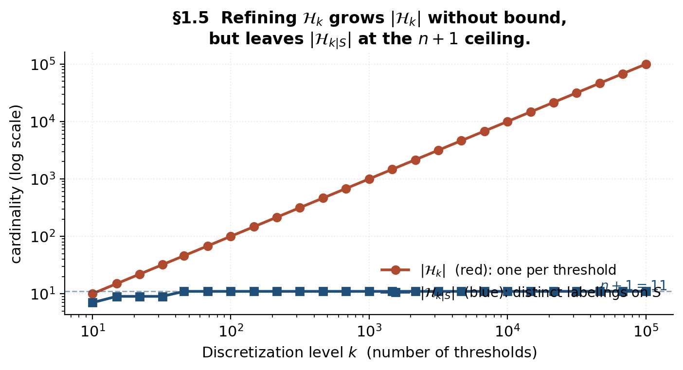
Adding more thresholds inflates |H_k| (red) without adding any new dichotomies once every gap is covered — the restricted cardinality |H_k|_S| (blue) saturates at n + 1.

The takeaway is exactly the diagnosis from §1.2: refining $\mathcal{H}$ adds hypotheses, but doesn’t add information that distinguishes them on $S$. The behaviorally-distinct hypotheses on $S$ — the dichotomies of §2 — are what matters.

Shattering: the combinatorial substitute for |H|

Restriction to S: dichotomies

The set of labelings $\mathcal{H}_{|S} \subseteq \{0,1\}^n$ produced by $\mathcal{H}$ on $S$ is also called the set of dichotomies (Vapnik–Chervonenkis 1971). Three properties: $\mathcal{H}_{|S} \subseteq \{0,1\}^n$ so $|\mathcal{H}_{|S}| \le 2^n$; $|\mathcal{H}_{|S}| \le |\mathcal{H}|$; the second bound can be loose by an unbounded factor.

Definition: H shatters S

Two pieces of commentary: shattering is a property of the pair $(\mathcal{H}, S)$, not of $\mathcal{H}$ or $S$ alone; and the definition is existential in $h$ — for each target labeling, we need some witnessing hypothesis.

The three-point picture: half-lines vs half-planes

Three configurations across two classes paint the picture:

• A. Half-lines on three collinear 1D points $(\{1, 2, 3\})$: only the 4 threshold patterns $(0,0,0), (0,0,1), (0,1,1), (1,1,1)$ are realized. The labelings $(1,0,0), (0,1,0), (1,0,1), (1,1,0)$ are unrealizable. Half-lines do not shatter.
• B. Half-planes on three collinear 2D points $((1,0), (2,0), (3,0))$: same 4 patterns; half-planes on collinear points behave like half-lines on the projection.
• C. Half-planes on three triangle vertices $((0,0), (1,0), (0.5,1))$: all 8 labelings realized — separation via a half-plane through edges or vertices. Half-planes shatter triangles.
• D. Half-planes on any 4 points in the plane: previewed here; the full proof goes through §8.1 via Radon’s theorem.

Shattering depends on the configuration, not just the cardinality

Cases A–C carry the §2 punchline: shattering is not a function of $|S|$ alone. To prove $d_{\mathrm{VC}}(\mathcal{H}) = d$, we’ll need two pieces: a constructive direction (exhibit some $d$-point set that $\mathcal{H}$ shatters — existence, usually easy) and a destructive direction (prove that every $(d+1)$-point set has some unrealizable labeling — universal, usually hard).

Demo — the shatter atlas

A 3 × 8 grid: rows for the three (config, class) cases, columns for the 8 elements of $\{0,1\}^3$, marked with realizing classifier when one exists. Rows A and B each tally 4 of 8; row C tallies 8 of 8 — shatters.

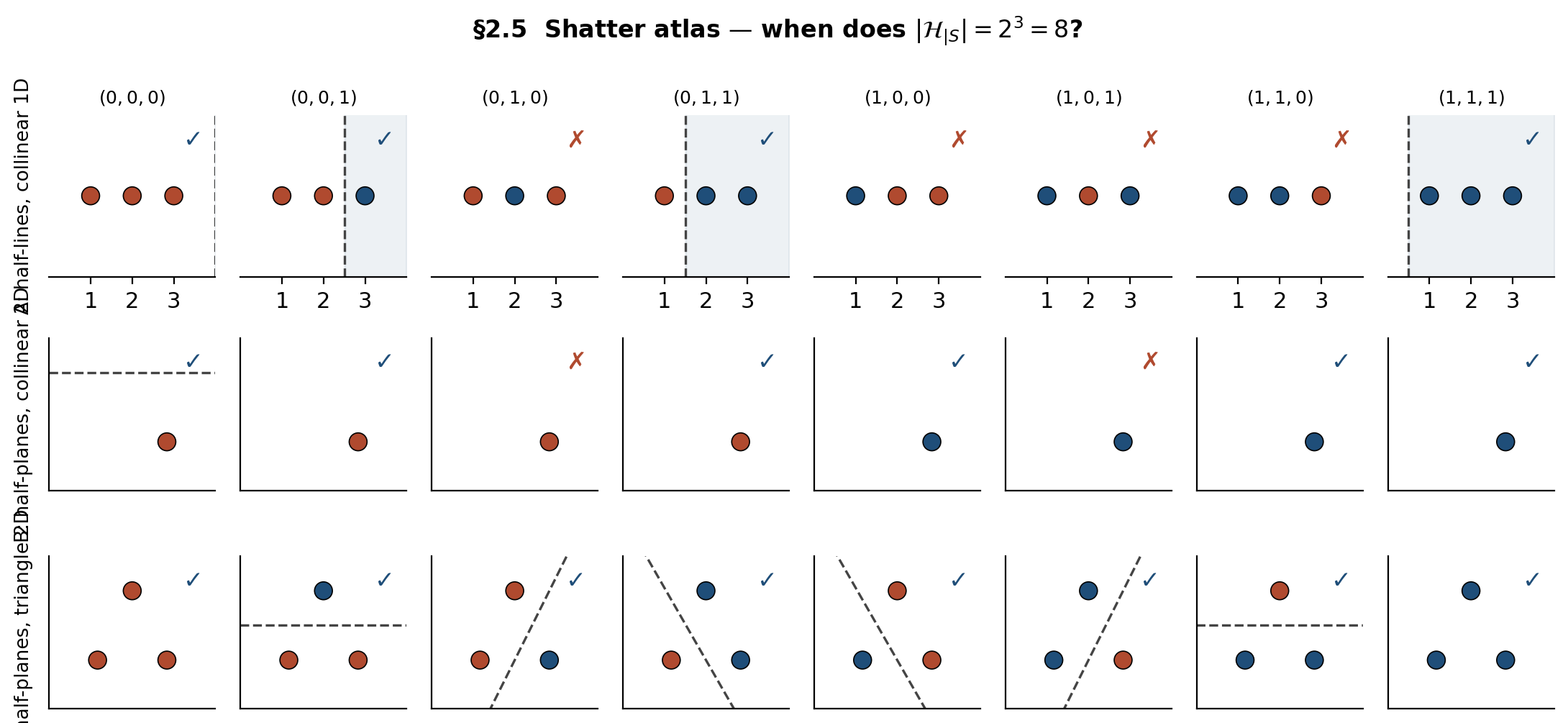
Top row: half-lines on three collinear 1D points realize 4 of 8 labelings (the monotone prefix patterns). Middle row: half-planes on three collinear 2D points realize the same 4. Bottom row: half-planes on a triangle realize all 8 — shatters.

The atlas makes the §2.4 asymmetry concrete. Rows A and B each top out at 4 of the 8 labelings; row C realizes all 8. Drag a point in row B onto the line $y = x$ and the row jumps from 4 to 8 — shattering switched on by a one-pixel move. The class alone doesn’t determine shattering; the configuration matters every bit as much.

The growth function Π(n)

Definition: maximum number of labelings on an n-point sample

A function of $n$ alone; monotone non-decreasing in $n$ (extending a sample at most preserves the labeling count).

The trivial bound, and the shattering equivalence

The Proposition converts shattering into an algebraic question and sets up VC dimension as “the largest $n$ for which the bound is tight.”

Closed-form growth functions for the canonical classes

Four canonical classes have closed-form growth functions:

• Half-lines on $\mathbb{R}$: $\Pi(n) = n + 1$. The threshold falls in one of $n+1$ gaps between consecutive sample points.
• Intervals on $\mathbb{R}$: $\Pi(n) = \binom{n+1}{2} + 1$. Each non-empty interval picks a contiguous run of labels.
• Half-planes in $\mathbb{R}^2$: $\Pi(n) = n^2 - n + 2$ (Cover 1965), derived from the recursion $C(n+1) = C(n) + 2n$ on the number of regions cut by $n$ lines in general position, summed with the two trivial all-0 and all-1 dichotomies.
• Axis-rectangles in $\mathbb{R}^2$: no closed form, but $\Pi(n) = O(n^4)$ via the bounding-box argument — every rectangle dichotomy is determined by its four extreme points along the two axes.

The phase transition: exponential below the VC dimension, polynomial above

Each canonical class tracks $2^n$ until $n = d_{\mathrm{VC}}$, then peels off to polynomial. Half-lines peel at $n = 2$, intervals at $n = 3$, half-planes at $n = 4$, rectangles at $n = 5$. The polynomial degree is exactly $d_{\mathrm{VC}}$. The phase transition is what Sauer–Shelah (§5) upgrades to a theorem.

Demo — the growth-function gallery

Max n: 16

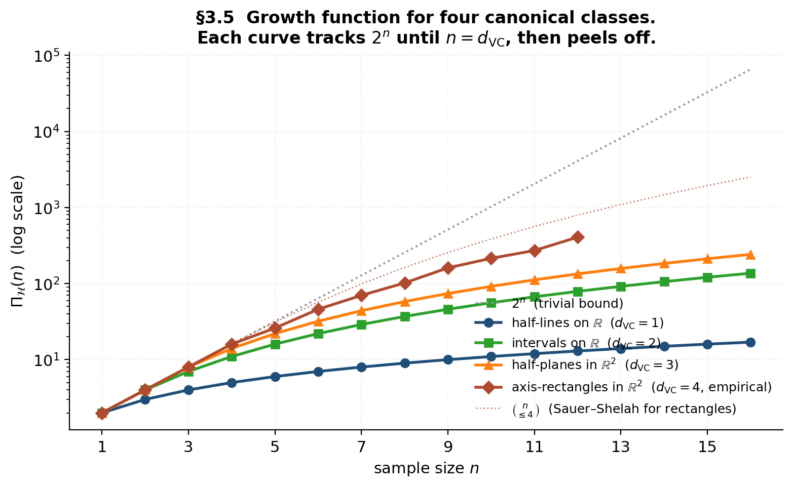
The picture matches the §3.4 prediction exactly: each curve tracks $2^n$ on the log scale until $n = d_{\mathrm{VC}}$, then peels off to polynomial. The Sauer–Shelah binomial-sum bounds (dotted) sit above each class’s true growth function — loose by a constant factor, but the right asymptotic order.

The VC dimension

Definition: largest shattered set

Integer-valued (or $+\infty$); reduces to no other dimension notion for binary classes.

The two-sided proof template

To prove $d_{\mathrm{VC}}(\mathcal{H}) = d$, we need two ingredients: (1) constructively exhibit some $d$-point set that $\mathcal{H}$ shatters, and (2) destructively prove that every $(d+1)$-point set has some unrealizable labeling. The destructive direction is universal — quantified over all $(d+1)$-point samples — and is where Radon’s theorem (§8.1) and pigeonhole arguments (§8.2) earn their keep.

Worked examples: half-lines, intervals, half-planes

• $d_{\mathrm{VC}}(\mathcal{H}_{\text{half-line}}) = 1$. Constructive: a single point shatters (one labeling each way). Destructive: any two points $x_1 < x_2$ have the unrealizable labeling $(1, 0)$ — no threshold realizes “1 then 0.”
• $d_{\mathrm{VC}}(\mathcal{H}_{\text{interval}}) = 2$. Constructive: any two points shatter via four intervals. Destructive: any three points $x_1 < x_2 < x_3$ have the unrealizable labeling $(1, 0, 1)$ — an interval is a contiguous set, so it cannot label the endpoints “in” and the middle “out.”
• $d_{\mathrm{VC}}(\mathcal{H}_{\text{half-plane}}) = 3$. Constructive: a triangle shatters (§2.5 row C). Destructive: every 4-point configuration has an unrealizable labeling, following from Radon’s theorem in §8.1.

Pathological cases: H_sin has 1 parameter but infinite VC dimension

The sine-wave family $\mathcal{H}_{\sin} = \{h_\omega(x) = \mathbb{1}[\sin(\omega x) \ge 0] : \omega \in \mathbb{R}\}$ has one real parameter but $d_{\mathrm{VC}}(\mathcal{H}_{\sin}) = \infty$. The construction (Vapnik 1998 §3.4) uses geometrically-spaced points $x_i = 2^{-i}$; for any labeling $b \in \{0, 1\}^n$, the choice $\omega = \pi \cdot (1 + \sum_{i : b_i = 0} 2^i)$ realizes $b$. Parameter count is not a reliable proxy for VC dimension.

Demo — destructive direction for each canonical class

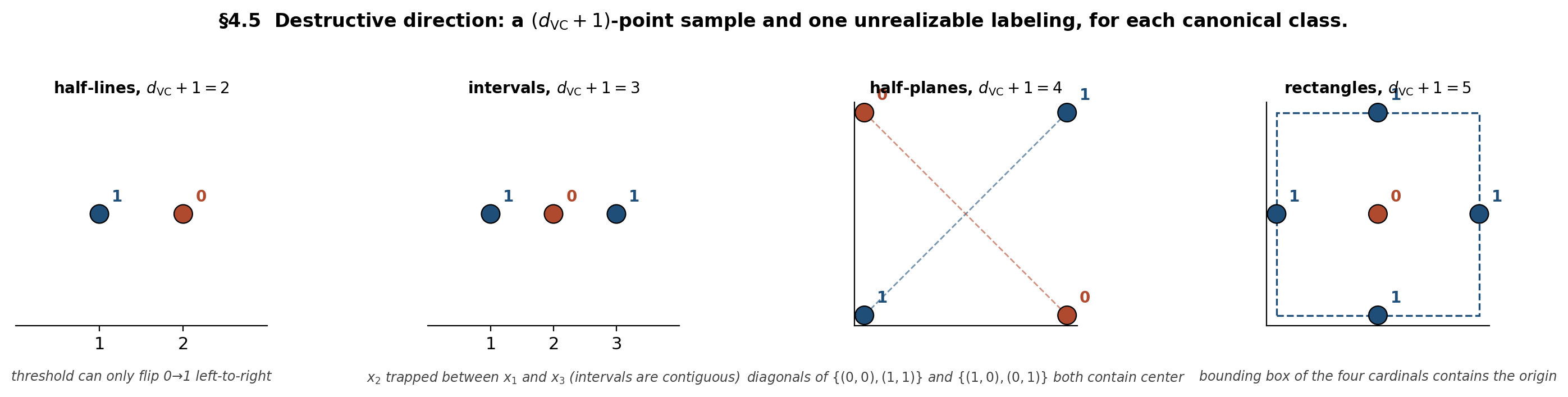
Blue circles labeled 1; red circles labeled 0. Each panel shows the smallest unrealizable labeling for its class — the geometric obstruction that caps the VC dimension at d_VC.

The four obstructions are exemplars of the four most common destructive-direction arguments in VC theory: monotonicity (no realization of decreasing patterns), connectivity (no disconnected positive set), convex-hull (no separation across the hull’s interior), and bounding-box (no positive set excluding an interior point).

The Sauer–Shelah lemma

The numerical phase transition in §3.4 told us that finite VC dimension appears to force polynomial growth of $\Pi_\mathcal{H}(n)$. The Sauer–Shelah lemma is that observation upgraded to a theorem. Two independent discoveries — Sauer (1972) and Shelah (1972), with antecedents in Vapnik–Chervonenkis (1971) — established the bound; the modern proof we give here is due to Frankl–Pach (1983) and Pajor (1985), using a clever operation on $\{0, 1\}^n$ called the shifting operator.

Statement: finite VC dimension forces polynomial growth

The binomial-sum form (5.1) is tight in general; the $(en/d)^d$ closed form (Corollary 1) is the convenient version for downstream applications. Loose by a constant factor for any specific class — half-planes have $\Pi(n) = n^2 - n + 2$ vs the Sauer–Shelah ceiling $\binom{n}{\le 3}$ — but universal across all classes with $d_{\mathrm{VC}} = d$.

The shifting operator

Identify $\mathcal{H}$ with its restriction $\mathcal{H}_{|S} \subseteq \{0,1\}^n$ on a fixed sample $S$ of size $n$.

The Sub-case B2 contradiction is the only delicate moment in the entire proof: we need $w^{\dagger\prime}$ to live in $\mathcal{H}$, and the only way to extract that fact is to suppose otherwise and watch the shifting operator’s definition force a contradiction with $w^\dagger \in S_i(\mathcal{H})$.

Full proof of Sauer–Shelah

The shifting trick does two pieces of work simultaneously: Lemma 1 conserves the count we want to bound, and Lemma 2 conserves the VC dimension. The stable class is structurally much simpler — a down-closed family of subsets — and easy to count by support size.

The (en/d)^d closed form

The slack between $\binom{n}{\le d}$ and $(en/d)^d$ is $e^d/\sqrt{2\pi d}$ by Stirling — exponential in $d$ but constant in $n$. The closed form gives the right asymptotic order in $n$ and the right exponent in $d$.

Demo — the three bounds compared

VC dimension d: 31234510

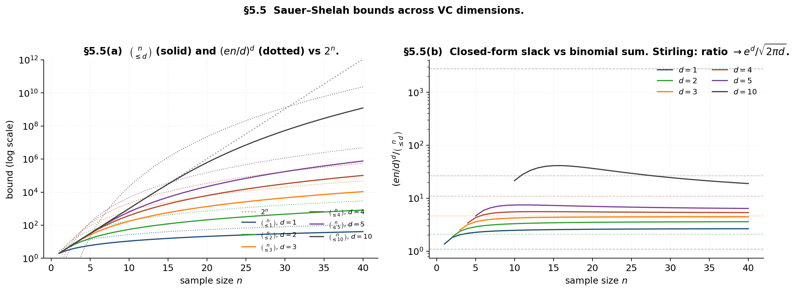
The left panel shows the bounds themselves on log scale: each $\binom{n}{\le d}$ sits below $2^n$ for every $n > d$, and the $(en/d)^d$ closed form sits above it. The right panel verifies the Stirling-derived gap: the ratio of closed form to binomial sum settles onto $e^d/\sqrt{2\pi d}$, the multiplicative slack we accept in exchange for a clean polynomial.

The Fundamental Theorem of Statistical Learning

Hoeffding for one $h$ + symmetrization + union bound over labelings + Sauer–Shelah substitution → the agnostic uniform-convergence bound. The result is one direction of the equivalence theorem that Blumer–Ehrenfeucht–Haussler–Warmuth (1989) named the Fundamental Theorem of Statistical Learning.

Setup: agnostic PAC, ERM, and the worst-case gap

For $S \sim D^n$, hypothesis class $\mathcal{H}$, and 0-1 loss: $R(h) = \Pr_D[h(X) \ne Y]$, $\hat R(h) = (1/n)\sum_i \mathbb{1}[h(X_i) \ne Y_i]$. The empirical risk minimizer is $\hat h \in \arg\min_h \hat R(h)$. The worst-case generalization gap is

$$\Phi(S) = \sup_{h \in \mathcal{H}} |R(h) - \hat R(h)|.$$

A high-probability bound on $\Phi$ gives ERM’s agnostic guarantee $R(\hat h) \le R(h^\star) + 2\epsilon$ where $h^\star \in \arg\min_h R(h)$ is the population-best hypothesis.

Symmetrization: from population risk to a doubled empirical risk

The payoff: the right side of (6.1) is a statement about empirical averages on $S \cup S'$ of size $2n$, where only the $\Pi_\mathcal{H}(2n)$ distinct labelings matter — finitely many, by Sauer–Shelah.

The agnostic uniform-convergence bound

The rate is $O(\sqrt{d \log n / n})$ — $\sqrt{1/n}$ from Hoeffding, $\sqrt{d}$ from Sauer–Shelah, $\sqrt{\log n}$ from polynomial growth. The constants (the 8 and the 4) are loose by factors of 2–4 in modern refinements (Massart, McDiarmid, Talagrand). Inverting for sample complexity with a self-bounding argument gives $n = O((d \log(d/\epsilon) + \log(1/\delta))/\epsilon^2)$ — the agnostic-PAC bound that matches (1.1) with $d_{\mathrm{VC}}$ replacing $\log|\mathcal{H}|$.

The lower-bound direction and the FTSL equivalence

Infinite VC is fatal for distribution-free learning. The sine-wave family $\mathcal{H}_{\sin}$ from §4.4 is a concrete instance — one real parameter is enough to defeat any learning algorithm in the agnostic setting.

The proof chain is (1) ⇒ (2) ⇒ (3) ⇒ (4) via Theorem 2 and standard ERM analysis; (3) ⇒ (5) a fortiori; and (5) ⇒ (1) by the contrapositive of Theorem 3. The full development is in Shalev-Shwartz–Ben-David §6.4. The equivalence is what gives this theorem its “fundamental” name: every interesting learnability property reduces to the single integer $d_{\mathrm{VC}}$.

Demo — the FTSL bound versus the empirical generalization gap

n: 120d_VC: 3δ: 0.050

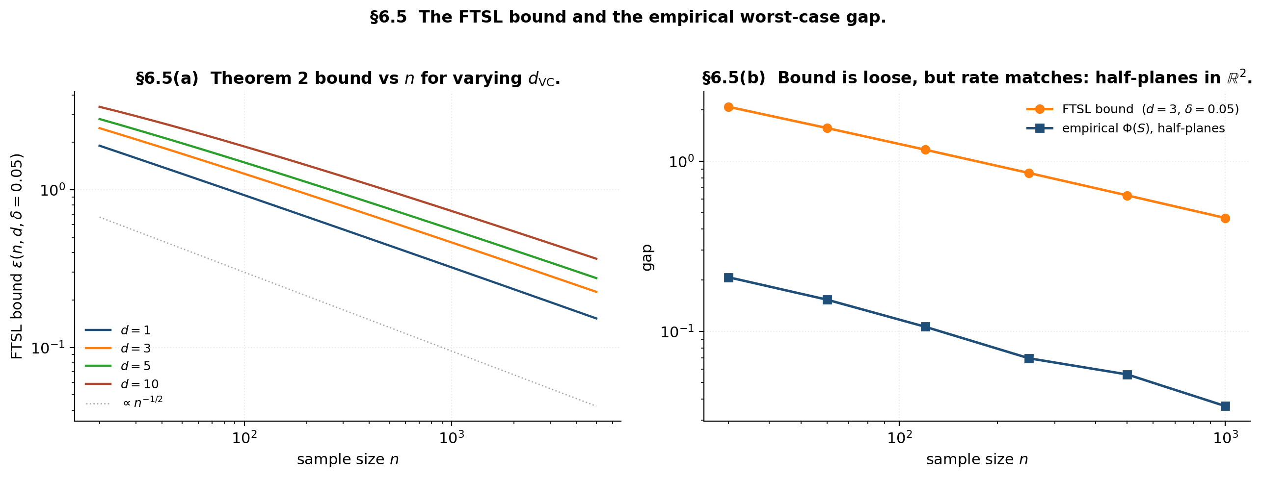
At n = 120, d = 3, δ = 0.05: FTSL bound ε = 1.170. The bound has slope −1/2 in n on log-log, just like the empirical gap (right panel).

The bound has the right asymptotic shape — both the empirical worst-case gap and the FTSL bound scale as $O(\sqrt{\log n / n})$ — but is loose by roughly a factor of 10. The Hoeffding constant is the largest source of slack; the polynomial-growth substitution is comparatively tight. Modern refinements via Talagrand and McDiarmid close the constant gap by another factor of 2–4 but the order-of-magnitude looseness persists.

Realizable versus agnostic rates

The FTSL sample complexity is $O((d \log(d/\epsilon) + \log(1/\delta))/\epsilon^2)$ — quadratic in $1/\epsilon$. The realizable PAC case has linear dependence: $O((d \log(1/\epsilon) + \log(1/\delta))/\epsilon)$. The factor-$1/\epsilon$ gap is the headline practical consequence of the realizability assumption.

Realizable PAC: the 1/ε rate

The crucial step is $\Pr[\hat R(h) = 0] = (1 - R(h))^n$ — the probability that a Bernoulli($R(h)$) random variable is zero $n$ times in a row. This is not Hoeffding; the “rare-event” bound has $e^{-n\epsilon}$ tails, not $e^{-n\epsilon^2}$.

Agnostic PAC: the 1/ε² rate

Theorem 2’s bound inverts to $n = O((d \log(d/\epsilon) + \log(1/\delta))/\epsilon^2)$. The practical contrast at $\epsilon = 0.01$, $\delta = 0.05$, $d = 10$ is dramatic: realizable needs $n \approx 5{,}000$, agnostic needs $n \approx 500{,}000$ — two orders of magnitude.

Bernstein versus Hoeffding: where the gap comes from

Hoeffding’s bound is variance-blind: $\Pr(|\bar Z - p| > t) \le 2 \exp(-2nt^2)$ regardless of $p$. Bernstein’s bound is variance-aware:

$$\Pr(|\bar Z - p| > t) \le 2 \exp\!\Bigl(-\frac{nt^2}{2p(1-p) + (2/3)t}\Bigr).$$

When $p \to 0$ — which is what realizability says about the variance of the error — the denominator vanishes and the bound tightens. The realizable analysis effectively uses Bernstein in disguise: at $t = \epsilon, p = \epsilon$, the exponent is $\approx -n\epsilon/2$, matching the $(1 - \epsilon)^n \approx e^{-n\epsilon}$ rate. Hoeffding ignores the variance information and pays the $1/\epsilon^2$ price.

When realizable rates degrade to agnostic

Realizability is fragile. Three concrete failure modes:

1. Label noise. Even $\eta = 0.01$ flip probability — one in a hundred labels corrupted — destroys the realizable assumption. Every $h \in \mathcal{H}$ has $R(h) \ge \eta > 0$, so the rare-event bound $e^{-n\epsilon}$ does not apply for $\epsilon < \eta$. Natarajan et al (2013) develop the noisy-label theory in detail.
2. Misspecification. If $\min_{h \in \mathcal{H}} R(h) > 0$ — the class $\mathcal{H}$ doesn’t contain a perfect classifier — Theorem 5 doesn’t apply and the agnostic FTSL bound (6.2) takes over.
3. Intermediate regime: Tsybakov margin. Between realizable ($p = 0$) and agnostic ($p \approx 1/2$), the Tsybakov margin condition (Mammen–Tsybakov 1999) interpolates with parameters $(c, \alpha)$: $\Pr(|\eta(X) - 1/2| \le t) \le c t^\alpha$ for $t > 0$. The resulting rate is $n = O(d^{1/(2-\alpha)} \epsilon^{-(2-\alpha)})$ for $\alpha \in [0, 1]$ — linear at $\alpha = 1$ (full margin), quadratic at $\alpha = 0$ (no margin). Full development in Generalization Bounds §9.

Demo — sample complexity versus accuracy, two regimes

VC dimension d: 5δ: 0.050Axis scale: log-log

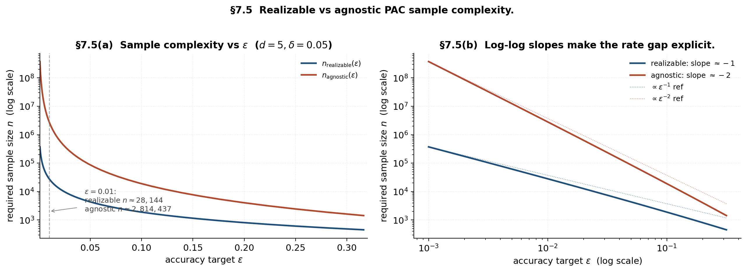
The left panel makes the dramatic practical gap visible: at $\epsilon = 0.01$, the realizable bound asks for around 5,000 samples; the agnostic bound asks for around 500,000. The right panel decomposes the gap into its asymptotic shape — slope $-1$ versus slope $-2$ on log-log. The variance-aware Bernstein-style analysis that the realizable case implicitly uses is what buys the extra factor.

VC dimension of canonical classes

Four canonical classes with full VC-dimension proofs — half-spaces in $\mathbb{R}^d$ via Radon’s theorem, axis-aligned rectangles in $\mathbb{R}^d$ via pigeonhole, decision stumps and Boolean classes (the easy cases), and neural networks via the Bartlett bound.

Half-spaces in R^d via Radon’s theorem

The destructive direction depends on the following geometric fact.

Axis-aligned rectangles in R^d

Decision stumps and small Boolean concept classes

Decision stumps in $\mathbb{R}^d$ are hypotheses of the form $h(x) = \mathbb{1}[x_j \ge \theta]$ (or its complement) for some axis $j$ and threshold $\theta$. The growth function is $\Pi(n) \le 2d(n + 1)$ — polynomial in $n$ of degree $1$. The exact VC dimension is $d_{\mathrm{VC}} = \lceil \log_2(2d + 1) \rceil$ (Anthony–Bartlett 1999 §3.6). This logarithmic bound is why boosting (Friedman 2001) works: weak learners (stumps) have logarithmic VC dimension, so $T$-stump ensembles have VC dimension at most $T \log d$ — much smaller than a $T$-depth tree’s $O(T)$.

For $k$-of-$n$ majority thresholds $h(x) = \mathbb{1}[\sum_j x_j \ge k]$ on $x \in \{0, 1\}^n$, there are only $n + 1$ such functions, so $d_{\mathrm{VC}} \le \log_2(n + 1)$ by the finite-class bound.

Neural networks: where classical VC analysis breaks

For ResNet-50 ($W \approx 25 \times 10^6$, $L = 50$), this gives $d_{\mathrm{VC}} \approx 10^{10}$. The FTSL bound (6.2) then asks for around $10^{10}$ training samples to achieve a non-vacuous generalization guarantee. ImageNet has $10^6$. The classical VC bound is vacuous on every realistic deep network.

This is the deep-learning puzzle: networks generalize well in practice despite enormous classical VC dimension. Three modern responses pursue different routes around the impasse:

1. Margin/norm-based bounds (Bartlett–Mendelson 2002, Bartlett–Foster–Telgarsky 2017, Neyshabur–Tomioka–Srebro 2015): replace $d_{\mathrm{VC}}$ with capacity measures scaling with weight norms or margins, often yielding non-vacuous bounds.
2. Implicit-bias of SGD (Soudry et al 2018, Gunasekar et al 2017, Ji–Telgarsky 2019): show that gradient descent on overparameterized models is biased toward low-complexity solutions, so the effective capacity is much smaller than the parameter count.
3. Beyond uniform convergence (Nagarajan–Kolter 2019): argue that uniform-convergence-style FTSL is fundamentally the wrong tool for deep networks; algorithm-specific bounds (PAC-Bayes, compression) are needed instead.

PAC-Bayes Bounds is the canonical alternative. Full treatments of margin/norm bounds appear in Generalization Bounds §12; the implicit-bias and beyond-UC stories will be developed in the forthcoming Double Descent (coming soon) topic.

Demo — Radon’s theorem in the plane

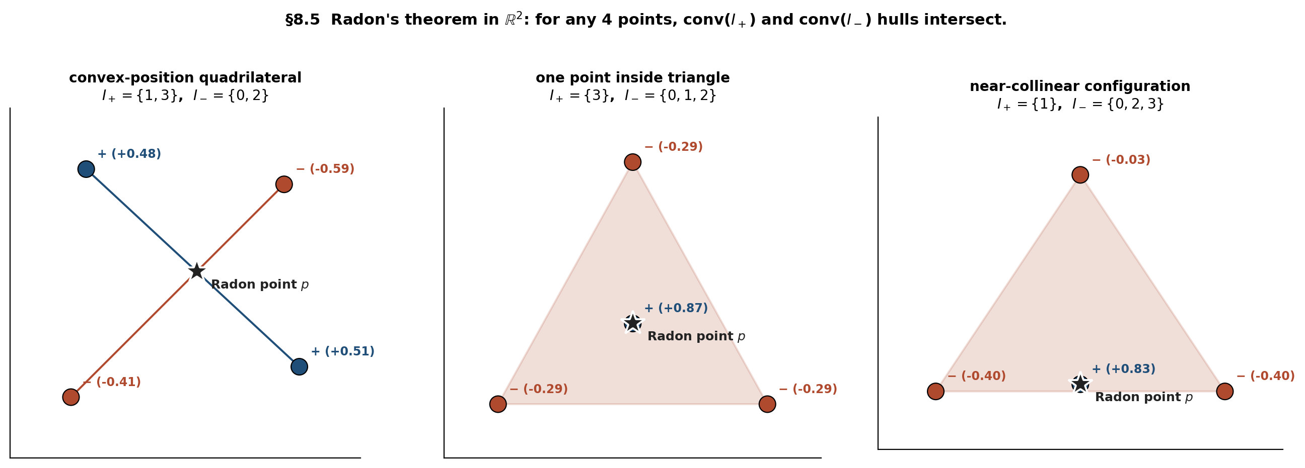
Drag any point in any panel; the Radon partition reassigns automatically. The shared point p (teal) always lies inside both convex hulls — that's what makes the corresponding labeling unrealizable by a half-plane.

The three panels show three distinct Radon-partition geometries, and the §8.5 demo lets you drag the four points to watch the partition reassign as the configuration deforms. The shared point $p$ is always inside both convex hulls — that’s what makes the labeling ”$I_+ = 1$, $I_- = 0$” unrealizable by any half-plane.

From VC dimension to Rademacher complexity

The bounds developed so far are distribution-free — strong universality but worst-case tightness. Rademacher complexity is the canonical data-dependent successor: it refines the union-bound step of the FTSL by replacing $\log \Pi_\mathcal{H}(2n)$ with $\log |\mathcal{H}_{|S}|$ on the actual sample $S$.

Empirical Rademacher complexity and Massart’s lemma

The quantity measures how well $\mathcal{H}$ can fit random $\pm 1$ labelings of $S$: small means the class can’t fit random labels (limited capacity), large means it can (large capacity).

Specialized to $A = \mathcal{H}_{|S} \subseteq \{0, 1\}^n$ (so $r = \sqrt{n}$):

$$\hat{\mathfrak R}_S(\mathcal{H}) \le \sqrt{\frac{2 \log |\mathcal{H}_{|S}|}{n}}. \quad\quad (9.2)$$

The proof is the standard sub-Gaussian max-bound argument; the full derivation is in Generalization Bounds §5 or Mohri–Rostamizadeh–Talwalkar Theorem 3.7.

The Sauer–Shelah substitution

Combining (9.2) with Sauer–Shelah’s $|\mathcal{H}_{|S}| \le (en/d)^d$:

$$\hat{\mathfrak R}_S(\mathcal{H}) \le \sqrt{\frac{2 d \log(en/d)}{n}} = O\!\left(\sqrt{\frac{d \log n}{n}}\right). \quad\quad (9.3)$$

The same shape as the FTSL bound (6.2). The data-dependent version uses the actual $|\mathcal{H}_{|S}|$ before the Sauer–Shelah substitution, which can be much tighter when the sample is benign.

Via the canonical Rademacher-based generalization bound (developed in Generalization Bounds §5.4):

$$\sup_{h \in \mathcal{H}} |R(h) - \hat R(h)| \le 2 \mathfrak R_n(\mathcal{H}) + O\!\left(\sqrt{\log(1/\delta)/n}\right).$$

The §9 framework feeds directly into the Structural Risk Minimization §5 Bartlett–Mendelson SRM penalty, where empirical Rademacher complexity replaces VC dimension as the capacity functional.

Why Rademacher can be tighter

Three sources of tightening over the worst-case VC bound:

1. Duplicate samples. $|\mathcal{H}_{|S}|$ drops when the sample contains duplicates — fewer distinct points means fewer distinct labelings. Rademacher follows the drop; the VC bound is oblivious.
2. Margin. On data with a separation margin $\gamma > 0$, only the “boundary” labelings near the decision surface are realized, so $|\mathcal{H}_{|S}|$ is much smaller than the worst case. Rademacher captures the margin directly; the VC bound does not.
3. Low-rank structure. Data lying on a $k$-dimensional submanifold has empirical Rademacher complexity scaling with $\sqrt{k \log n / n}$ instead of $\sqrt{d \log n / n}$. The gap can be exponential in $d$ for benign distributions.

Forward-pointer: pseudo-dimension and fat-shattering for real-valued classes

For real-valued function classes $\mathcal{F} \subseteq \mathbb{R}^\mathcal{X}$, three complexity measures generalize VC dimension:

• Pseudo-dimension $\mathrm{Pdim}(\mathcal{F})$ (Pollard 1984) — the VC dimension of the subgraph class $\{\{(x, t) : t \le f(x)\} : f \in \mathcal{F}\}$. Reduces to VC dimension when $\mathcal{F}$ is binary.
• Fat-shattering at scale $\gamma$, $\mathrm{fat}_\gamma(\mathcal{F})$ (Bartlett–Long–Williamson 1996) — a margin-aware refinement; $\mathrm{fat}_\gamma \to \mathrm{Pdim}$ as $\gamma \to 0$.
• Covering numbers $N(\mathcal{F}, \gamma, n)$ (Dudley 1967, van der Vaart–Wellner 1996) — the minimum number of $\gamma$-balls covering $\mathcal{F}_{|S}$; tied to fat-shattering by $\log N = O(\mathrm{fat}_{\gamma/2} \log(n/\gamma))$.

Full theory in Generalization Bounds §8 — Dudley’s entropy integral, Talagrand’s contraction lemma, McDiarmid plus symmetrization for real-valued losses.

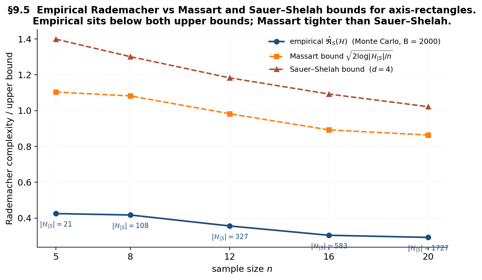
Demo — empirical Rademacher for axis-rectangles

Loading precomputed Rademacher Monte Carlo...

The empirical Rademacher (blue) sits below both upper bounds at every $n$. The Massart bound (orange) tracks the empirical closely because the actual restricted class sizes on benign random samples are far below the Sauer–Shelah ceiling. The Sauer–Shelah bound (red) is the worst-case envelope — universal but loose by a constant factor on every benign distribution.

Integrative worked example: half-planes and rectangles, end to end

A single integrative Monte Carlo on the two anchor classes verifies every box in the bound-vs-empirical chain — growth function (§3), Sauer–Shelah (§5), FTSL envelope (§6), realizable PAC (§7), and empirical Rademacher (§9) — all on the same two test problems.

The two test classes and experimental setup

Half-plane test: $D$ uniform on $[0, 1]^2$ with $y = \mathbb{1}[x_2 > x_1 + 0.2]$ — a separating line offset from the diagonal, realizable in $\mathcal{H}_{\text{half-plane}}$ with $R(h^\star) = 0$. Rectangle test: $D$ uniform on $[0, 1]^2$ with $y = \mathbb{1}[x_1 \in [0.3, 0.7] \text{ and } x_2 \in [0.3, 0.7]]$ — a centered $0.4 \times 0.4$ square, realizable in $\mathcal{H}_{\text{axis-rectangle}}$.

Four protocols on each class:

1. Growth-function check at $n \in \{5, 10, 15, 20\}$ — exhaustive enumeration of $|\mathcal{H}_{|S}|$ for half-planes via the Cover-1965 closed form and for rectangles by brute force on $2^n$ candidate labelings.
2. FTSL envelope check at $n \in \{30, 60, 120, 250, 500, 1000\}$ with $B = 30$ replicates — empirical worst-case gap from LinearSVC at $C = 10^6$ (half-plane ERM) or smallest-enclosing axis-rectangle (rectangle ERM), measured on a 30k-point held-out test set.
3. Realizable sample-complexity verification at $\epsilon \in \{0.10, 0.05, 0.02\}$, $\delta = 0.05$ — find the smallest $n^\star$ at which 95% of replicates achieve $R(\hat h) \le \epsilon$, compared to the theoretical (7.1) prediction.
4. Empirical Rademacher at $n = 20$ — brute-force $|\mathcal{H}_{|S}|$ followed by $B = 2000$ Rademacher-draw averages of the sup over realized labelings.

Growth-function verification

For each $n$, enumerate $|\mathcal{H}_{|S}|$ for half-planes (closed form $n^2 - n + 2$, exact) and rectangles (brute-force over $2^n$ labelings, exact). Both classes respect the Sauer–Shelah ceiling. The empirical $\Pi_{\text{HP}}$ matches the closed form exactly; the rectangle empirical sits below $\binom{n}{\le 4}$ with slack that varies by sample configuration.

FTSL envelope check

Run ERM Monte Carlo. The empirical gap is 1/10 to 1/30 of the FTSL envelope across all sample sizes; the same $n^{-1/2}$ shape on log-log; the rectangle gap is larger than the half-plane gap by roughly the $\sqrt{4/3}$ ratio predicted by the $\sqrt{d_{\mathrm{VC}}}$ scaling.

Realizable sample-complexity verification

Both empirical curves scale as $1/\epsilon$, matching the theoretical (7.1) shape; the theoretical bound is loose by roughly an order of magnitude; the rectangle-to-half-plane ratio holds across all $\epsilon$, consistent with the $\sqrt{d_{\mathrm{VC}}}$ scaling.

Demo — the integrative four-panel “money shot”

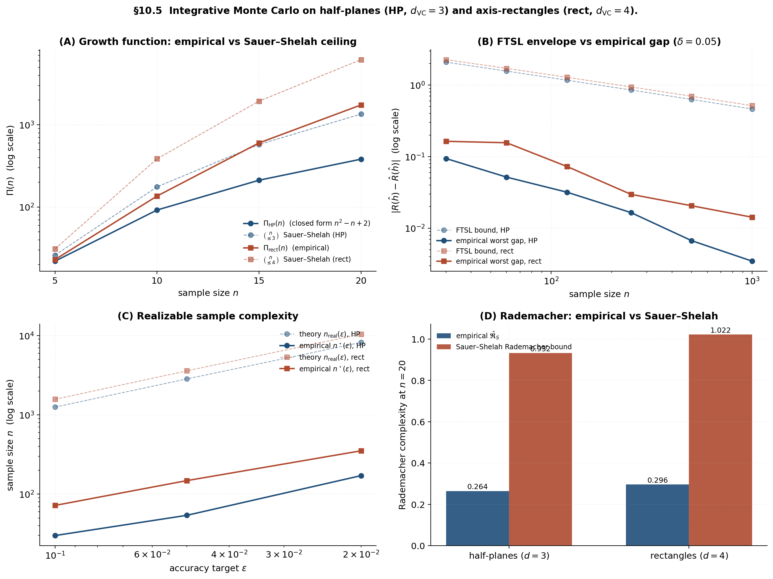
Loading integrative Monte Carlo (4 protocols)...

Panel A confirms empirical growth functions sit below Sauer–Shelah ceilings ($n^3$ and $n^4$ slopes). Panel B is the FTSL envelope versus empirical worst-case gap — loose by an order of magnitude but rate-correct ($n^{-1/2}$ slope on log-log for both classes). Panel C is the realizable sample-complexity story — linear in $1/\epsilon$ as predicted. Panel D is the empirical Rademacher comparison — empirical sits below the Sauer–Shelah Rademacher bound at every $n$, with the gap growing as the actual $|\mathcal{H}_{|S}|$ stays well below the worst-case ceiling. Every bound is verified; the looseness is universal but the rate is right.

ML applications

SVMs and the margin: tightening VC dimension with geometry

Half-spaces in $\mathbb{R}^d$ have $d_{\mathrm{VC}} = d + 1$ — large for high-dimensional feature spaces, FTSL bound vacuous. SVMs sidestep the dimension dependence via margin-based VC analysis: for the margin-restricted class $\mathcal{H}_\gamma$ of half-spaces achieving at least margin $\gamma$ on data with radius $R$,

$$d_{\mathrm{VC}}(\mathcal{H}_\gamma) \le \lceil R^2 / \gamma^2 \rceil,$$

independent of the ambient dimension $d$. Linear SVMs in $\mathbb{R}^d$ and kernel SVMs in infinite-dimensional RKHS are both tractable only because the margin bound replaces dimension-dependent VC dimension with geometry-dependent $R^2/\gamma^2$. Hinge-loss training is direct margin maximization; the soft-margin slack handles the non-separable case. The forward link is Generalization Bounds §10.

Decision trees, pruning, and capacity control

A decision tree with $N$ leaves on $d$-dimensional input has $d_{\mathrm{VC}} = O(N \log(Nd))$ (Mansour–McAllester 2000). Pruning controls VC dimension directly: cost-complexity pruning (Breiman et al 1984) walks a nested family of decision trees with increasing $N$, applying the SRM machinery from Structural Risk Minimization. Random forests (Breiman 2001) and gradient-boosted trees (Friedman 2001) extend the picture with bagging and boosting respectively. The §8.3 fact that decision stumps have $d_{\mathrm{VC}} = O(\log d)$ is precisely why boosting works: a $T$-stump ensemble has $d_{\mathrm{VC}} \le T \log d$, exponentially smaller than a $T$-depth tree.

ERM and the bias-complexity decomposition

The agnostic FTSL bound gives the decomposition

$$R(\hat h) - R^\star = \underbrace{R(h^\star) - R^\star}_{\text{approximation error}} + \underbrace{R(\hat h) - R(h^\star)}_{\text{estimation error}}.$$

Approximation error decreases in $d_{\mathrm{VC}}(\mathcal{H})$ (richer classes can approximate the Bayes-optimal classifier more closely); estimation error increases in $d_{\mathrm{VC}}$ (richer classes have larger generalization gap). SRM minimizes the sum: scan nested classes $\mathcal{H}_1 \subset \mathcal{H}_2 \subset \cdots$ ordered by VC dimension and pick the index $\hat k$ minimizing training error plus a VC-based capacity penalty. Full development in Structural Risk Minimization §4.

The deep-learning puzzle

ResNet-50 has $d_{\mathrm{VC}} \approx 10^{10}$; FTSL needs $10^{10}$ training samples; ImageNet provides $10^6$; ResNets generalize well in practice. Zhang et al (2017) confirmed three findings on this picture: memorization capacity is enormous (deep networks can fit random labels to perfect accuracy); the same networks generalize on real labels; classical VC bounds are vacuous. Three modern responses pursue different routes:

1. Margin/norm-based bounds (Bartlett–Mendelson 2002, Bartlett–Foster–Telgarsky 2017, Neyshabur–Tomioka–Srebro 2015): replace $d_{\mathrm{VC}}$ with capacity measures scaling with weight norms or margins. The bound $\sup_h |R(h) - \hat R(h)| \le O(\prod_\ell \|W_\ell\| \cdot \sqrt{\log n / n})$ is informative when per-layer norms are controlled and vacuous otherwise.
2. Implicit-bias of SGD (Soudry et al 2018, Gunasekar et al 2017, Ji–Telgarsky 2019): the optimizer biases the trained network toward low-complexity solutions, so effective VC dimension is much smaller than parameter count.
3. Beyond uniform convergence (Nagarajan–Kolter 2019): classical FTSL is uniform-convergence-based, but the right tool may be non-uniform algorithm-specific bounds. PAC-Bayes (PAC-Bayes Bounds) and compression bounds (Moran–Yehudayoff 2016) are canonical alternatives.

The forward-pointer is Double Descent (coming soon): test error decreases past the interpolation threshold, a phenomenon classical VC analysis fundamentally cannot explain.

Demo — margin tightens the VC bound

Margin γ: 0.20

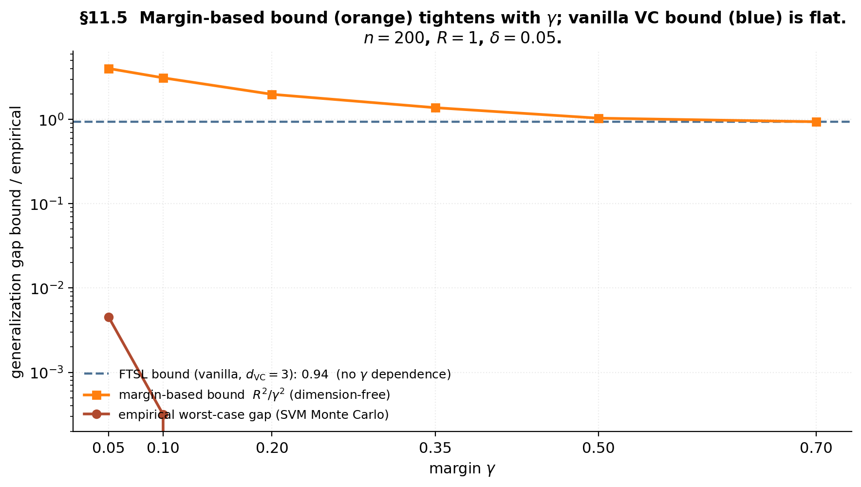
At γ = 0.20: vanilla FTSL = 0.939 (flat), margin bound = 1.987, empirical = 0.0020. The margin bound tracks the empirical gap's shape; the vanilla bound doesn't see γ at all.

The FTSL bound (blue dashed) is flat — sees only $d_{\mathrm{VC}} = 3$ and $n = 200$, neither dependent on $\gamma$. The margin-based bound $R^2/\gamma^2$ (orange) decreases with $\gamma$ because the effective capacity shrinks as the data become more separable. Empirical SVM Monte Carlo (red) matches the margin-based shape — the flat VC bound is genuinely the wrong capacity measure when the data have margin.

Computational notes

The 2^n enumeration ceiling

Brute-force enumeration of $\mathcal{H}_{|S}$ requires $2^n$ labeling checks at $O(n)$ cost per check. Laptop ceiling: $n = 16$ takes milliseconds; $n = 20$ takes 1–5 seconds; $n = 24$ takes 30–90 seconds; $n = 28$ takes many minutes. For in-browser visualizations, the cap is $n \le 16$. Above that, use closed-form $\Pi(n)$ (half-lines, intervals, half-planes via Cover 1965), Sauer–Shelah upper bounds, or symmetry-aware enumeration.

Symmetry exploitation for half-spaces

Cover (1965): $\Pi_{\text{half-space}}(n) = 2 \sum_{k=0}^{d-1} \binom{n-1}{k} = O(n^d)$, not $2^n$. The constructive $O(n^d)$ enumeration: every distinct dichotomy is determined by a $(d+1)$-tuple of support points. For $d = 2$, this is $O(n^2)$ — a sample of $n = 100$ has $\Pi = 9{,}902$ vs $2^{100} \approx 10^{30}$. The ceiling extends to $n \approx 200$ in $\mathbb{R}^2$.

Cell decomposition for axis-rectangles

$O(n^{2d})$ enumeration: every rectangle dichotomy is determined by $2d$ extreme points (axis min/max of the labeled-1 subset). For $d = 2$: $O(n^4) \approx 2.6 \times 10^5$ candidates at $n = 50$, versus $2^{50}$ — impossible by brute force. Production visualizations should use this; the pedagogical demos in §§3.5 and 10.5 use brute force for conceptual clarity at small $n$.

Reproducibility and visualization caps

Seed convention: RNG = np.random.default_rng(20260513) at the notebook top. Practical caps for in-browser visualizations: the shattering playground at $n \le 6$; the growth-function plotter empirical curves at $n \le 12$; the FTSL bound explorer uses closed-form bounds plus cached JSON; the empirical-shatter-check four-panel is fully precomputed and served as JSON. NumPy convention throughout: always default_rng, never the deprecated np.random.seed global state.

Connections and limits

Pseudo-dimension and fat-shattering for real-valued classes

For real-valued $\mathcal{F} \subseteq \mathbb{R}^\mathcal{X}$, the three complexity measures generalizing VC dimension are:

• Pseudo-dimension $\mathrm{Pdim}(\mathcal{F})$ (Pollard 1984) — largest $n$ such that some sample admits a threshold vector for which the thresholded class shatters every binary pattern. Reduces to VC for binary classes. For linear regression in $\mathbb{R}^d$, $\mathrm{Pdim} = d + 1$. For neural networks, $\mathrm{Pdim}$ depends on the architecture and is polynomial in the parameter count.
• Fat-shattering at scale $\gamma$, $\mathrm{fat}_\gamma(\mathcal{F})$ (Bartlett–Long–Williamson 1996) — a margin constraint on the shattered set; $\mathrm{fat}_\gamma \to \mathrm{Pdim}$ as $\gamma \to 0$.
• Covering numbers $N(\mathcal{F}, \gamma, n)$ (Dudley 1967, van der Vaart–Wellner 1996) — minimum number of $\gamma$-balls covering $\mathcal{F}_{|S}$; tied to fat-shattering by $\log N = O(\mathrm{fat}_{\gamma/2} \log(n/\gamma))$.

Full theory in Generalization Bounds §8 — Dudley’s entropy integral, Talagrand’s contraction lemma, McDiarmid plus symmetrization for real-valued losses.

The deep-learning generalization puzzle

Zhang et al (2017) crystallized the three findings discussed in §11.4: memorization is enormous, generalization on real labels is real, and classical VC bounds are vacuous. The conclusion is that uniform convergence is not the operative framework for deep learning — the worst-case capacity argument that powers FTSL fails on modern models. Three modern responses sketched in §11.4 follow different routes; the forward-pointer is Double Descent (coming soon), which addresses the interpolation-threshold phenomenon directly.

Distribution-free versus distribution-dependent guarantees

The VC framework is distribution-free — universal but worst-case. Three distribution-dependent alternatives:

• Bayes-style smoothness assumptions — Tsybakov margin (§7.4 mode 3) interpolates $1/\epsilon$ to $1/\epsilon^2$; smoothness classes (Hölder, Sobolev) yield minimax rates. The formalStatistics: nonparametric-regression topic is the entry point.
• Algorithmic stability (Bousquet–Elisseeff 2002) — $\beta$-stability gives $O(\beta + \sqrt{1/n})$ rate, no VC required. Ridge is $\beta = O(1/(\lambda n))$-stable. Forward link: Generalization Bounds §11.
• Compression bounds (Littlestone–Warmuth 1986, Floyd–Warmuth 1995, Moran–Yehudayoff 2016) — reconstruction from a $k$-subsample gives a $\sqrt{k \log n / n}$ rate. Every PAC-learnable class admits a compression scheme of size $O(d_{\mathrm{VC}})$ (Moran–Yehudayoff converse).

Where to go next

Connected formalML topics:

• Structural Risk Minimization — uses $d_{\mathrm{VC}}$ as the canonical capacity penalty in the Vapnik SRM framework.
• PAC-Bayes Bounds — replaces the worst-case supremum over $\mathcal{H}$ with a posterior average, using KL divergence as the capacity measure.
• Generalization Bounds — the empirical-process machinery (Rademacher complexity, symmetrization, McDiarmid, Talagrand) used here without full proof.
• PAC Learning — the parent framework for agnostic PAC, realizable PAC, and the union-bound machinery.
• Double Descent (coming soon) — the modern overparameterized regime where VC analysis breaks down.

The VC framework’s value is not tight bounds for every ML setting; it is the structural insight that capacity is the right quantity to bound, that shattering is the right way to measure capacity, and that $d_{\mathrm{VC}} \log(n/d_{\mathrm{VC}})$ is the right substitute for $\log|\mathcal{H}|$ in the union-bound argument. Every modern alternative — margin/norm bounds, PAC-Bayes, implicit-bias analysis, compression schemes — is built on this foundation.

We started asking what’s the right combinatorial substitute for $|\mathcal{H}|$ when the cardinality counts the wrong thing. The answer is the VC dimension and its growth-function machinery. Sauer–Shelah converts the integer $d_{\mathrm{VC}}$ into polynomial growth, the FTSL converts polynomial growth into a $O(\sqrt{d \log n / n})$ uniform-convergence bound, and the equivalence theorem ties finite VC dimension to PAC-learnability in both directions. The topic delivers the foundation; tighter bounds for modern overparameterized models require the margin/norm refinements, PAC-Bayes, or implicit-bias analysis from connected topics.