Causal Inference Methods
Identification, doubly-robust estimation, and inference under confounding — from potential outcomes and IPW through AIPW, TMLE, and DML, with instrumental variables, front-door identification, heterogeneous treatment effects, and sensitivity analysis
§1 Motivation: prediction is not enough
A trained-and-tested machine-learning model that predicts well on held-out data is a wonderful thing. It tells us — with quantified uncertainty, even — what we should expect to see when a fresh covariate vector arrives at deployment. It does not, in general, tell us anything about what would happen if we intervened to change . Those are different questions, and the distinction is the whole reason this topic exists.
This section establishes the distinction concretely, surveys the standard pathologies of naive adjustment, sketches the rest of the topic, and previews the running example we’ll thread through every estimator. The arc is short: predictive estimands measure associations in a distribution; causal estimands measure effects of interventions; under the right assumptions the two coincide; and the methods we’ll develop are recipes for moving from association to effect when those assumptions hold.
Statistical estimands vs causal estimands. Let be a binary treatment, a real-valued outcome, and a vector of pre-treatment covariates we observe. Two estimands sit close together in notation and very far apart in meaning:
The first is a contrast of conditional means in the observed-data distribution — a statistical estimand, computable from any iid sample by replacing each with a sample average. The second is a contrast of expected potential outcomes : the values would take if every unit were forced into treatment (resp. control). Those potential outcomes are counterfactual — for any given unit we observe only one of them, namely — so the second estimand cannot, in general, be read off the observed-data distribution without further assumptions. We unpack that machinery in §2 (notation) and §3 (assumptions). For now, take it on faith that is the object of interest and is its statistical doppelgänger.
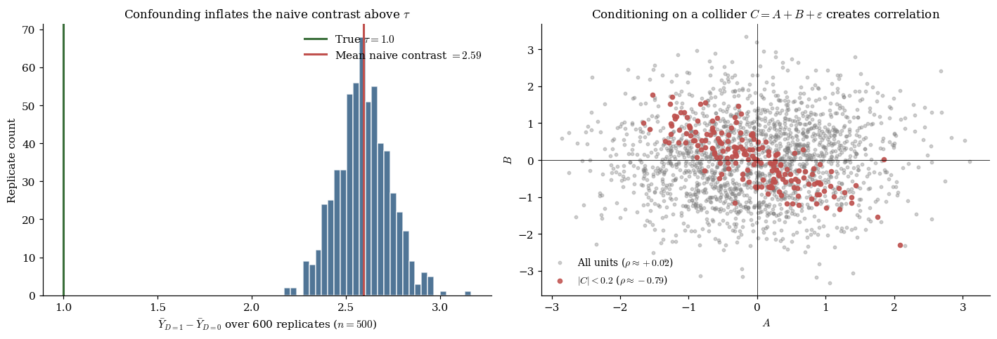
The two estimands agree in randomized experiments, where treatment is assigned independently of : randomization severs the link that would otherwise let drive both and simultaneously. They disagree in observational data — sometimes by a lot. A treatment that looks like it works because sicker patients are the ones who receive it can produce , apparently harmful, when , actually beneficial. That sign-flip is the bias the rest of this topic is built to retire.
When “controlling for ” goes wrong. The textbook prescription — adjust for all variables that affect both and — is correct in spirit and easy to get wrong in practice. Two mistakes are common enough to deserve names.
Colliders. A collider is a variable that is a common effect of two others. Conditioning on a collider — say, by adding it as a regressor — opens a path between its parents that was not there before. The cleanest example: take and as independent standard normals and let be a noisy sum. Marginally, . Conditional on , the only way to have is to have , so is sharply negative. We have manufactured a dependence by adjusting for a variable we should have left alone.
Mediators. A mediator sits on a causal path from to — treatment causes the mediator, the mediator causes the outcome. Adjusting for a mediator subtracts out part of the very effect we want to measure, leaving only the direct portion. This is sometimes exactly what we want (controlled-direct-effect questions) and sometimes catastrophic (when the total effect is the thing that matters). The mistake is symmetric to the collider one: the textbook rule “control for ” is not a license to control for every .
The lesson is not “adjust less” or “adjust more.” It is adjust correctly — which requires knowing enough of the causal structure to identify confounders without sweeping up colliders or mediators. §2 makes this precise via potential outcomes; §3 makes it precise via d-separation on DAGs.
Map of the topic. The topic is organized along the identification-and-confounding-control axis: given an estimand, what assumptions let us recover it from observed data, and what estimators implement that recovery efficiently? §§2–3 build the framework — potential outcomes, ignorability, positivity, the identification theorem. §§4–8 develop estimators that assume ignorability: IPW (§4), outcome regression and the g-formula (§5), augmented IPW (§6), targeted maximum likelihood (§7), and double machine learning (§8). The pedagogical arc is that each new estimator improves on its predecessors by being more robust to nuisance-model misspecification, culminating in DML, which licenses arbitrary off-the-shelf ML nuisance fits while preserving -asymptotic inference. §§9–10 handle the case where ignorability is unavailable: instrumental variables and front-door identification. §§11–12 cover heterogeneous treatment effects and sensitivity to unmeasured confounding. §13 threads the running example through every estimator end-to-end, and §14 closes with limits and connections.
The signature theorem of this topic is the doubly-robust property of AIPW (§6.2): AIPW is consistent for whenever either the propensity model or the outcome model is correctly specified — a remarkable two-shots-on-goal guarantee no single-model estimator can match. The doubly-robust property is the bridge from the §§4–5 single-model estimators to the §§7–8 machinery that lets us use modern ML for nuisance estimation.
The running example. Throughout the topic we work with a partially-linear data-generating process in the Robinson (1988) tradition:
with , independent of , smooth nonlinear outcome confounder , smooth nonlinear propensity score , and known true ATE . The concrete forms we use are
where is the logistic sigmoid and the standard normal CDF. Propensity is coupled to the outcome via (the same variable that drives the nonlinear component of ); without this coupling, the naive contrast would be unbiased and the §5 misspec demonstration would fail to land. The DGP is benign enough that closed-form intuition is available, but rich enough that lasso, random-forest, and OLS nuisance fits give qualitatively different downstream behavior — which is exactly what we need to make the §6–§8 robustness story visible.
§2 The potential-outcomes framework
§1 introduced the causal estimand without defining the notation. This section unpacks it: what means, what assumptions make it well-defined, why we can never observe it directly, and how the various target estimands of causal inference (ATE, ATT, CATE) relate. The framework we adopt is the Neyman–Rubin potential-outcomes framework, due to Neyman (1923) and elevated to general statistical use by Rubin (1974). The DAG-based framework of Pearl reappears in §3 and §10; for setting up notation, potential outcomes are cleaner.
Counterfactual notation. For each unit , the potential outcomes are and — the values of the outcome that would obtain if unit received control () or treatment (), respectively. We treat as fixed, unit-level attributes — properties of the unit, not random variables associated with the experiment. Randomness enters through treatment assignment and through whatever measurement error or post-treatment noise is built into the outcome. The unit-level treatment effect is . This is the quantity we would want to know for each unit if we could observe both potential outcomes. In reality we observe only , the realized outcome under the assigned treatment, and never the counterfactual .
Definition 1 (SUTVA, consistency, ATE).
The Stable Unit Treatment Value Assumption (SUTVA; Rubin 1980) requires both no interference — unit ‘s potential outcomes depend on ‘s own treatment, not on other units’ treatments — and no hidden treatment versions — each value corresponds to a single well-defined intervention. Under SUTVA the consistency identity is definitional:
The average treatment effect is ; the ATT is ; and the conditional average treatment effect is . The three are linked by and .
The fundamental problem of causal inference. The defining difficulty of causal inference is that for each unit we observe but never . The unit-level effect is unobservable. Holland (1986) named this the fundamental problem of causal inference, and it is genuinely a problem — not a technical detail to be waved away. Standard statistical inference deals with missing data as a contingent feature of the sampling design; here, the missing data is structural — half of every potential-outcome pair, every time.
The way out is to give up on unit-level effects and aim for averages over the population. The estimand is an average over the population’s unit-level effects, not a unit-level quantity. Under the assumptions of §3, those averages can be expressed as functionals of the observed-data distribution despite the structural missingness.
§3 Identification under ignorability and positivity
§2 set up the potential-outcomes notation and showed why unit-level effects are unobservable. The next question is when averages of those unit-level effects can be recovered from observed-data quantities. The answer comes in three pieces: a structural condition (ignorability), a regularity condition (positivity), and a theorem that exhibits the ATE as two distinct functionals of the observed-data distribution — one a propensity-weighted contrast, the other a covariate-adjusted regression contrast. These two representations are the seeds of the §4 IPW estimator and the §5 outcome-regression estimator, respectively.
Definition 2 (Ignorability and positivity).
Conditional ignorability (no unmeasured confounding, conditional exchangeability) is
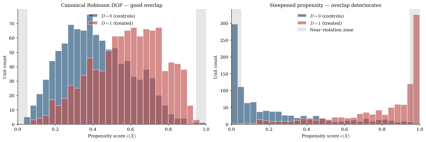
Positivity (overlap) is a.s., where the propensity score is .
Ignorability is a substantive assumption about the data-generating process. It holds, by construction, when contains every variable that simultaneously affects both treatment assignment and potential outcomes. There is no statistical test for ignorability from observed data alone; the field treats it as a structural claim defended on substantive grounds (study design, domain knowledge, sensitivity analysis — §12). Positivity is a regularity condition that makes and finite. Practical positivity violations — where is technically bounded but lives close to on a non-trivial mass of — are a frequent cause of trouble in real applied work.
Randomized experiments. The cleanest setting where both ignorability and positivity hold by construction is a randomized experiment. If unconditionally and , then ignorability holds trivially with any and positivity holds because the propensity is just the fixed assignment probability. Everything we develop in §§4–10 is in some sense machinery for approximating the conditions of a randomized experiment when randomization is impossible — by reweighting (IPW), by regression adjustment (g-formula), by augmentation (AIPW), or by instrumental-variable manipulation (IV).
Theorem 1 (Identification of the ATE).
Assume SUTVA, consistency, ignorability , and positivity a.s. Then the ATE is identified by both:
(a) The g-formula (standardization) functional:
(b) The inverse-probability-weighting (IPW) functional:
Proof.
We show (a): for each ; the ATE follows by taking the difference. The three-step chain is iterated expectation → ignorability → consistency:
The second line is the load-bearing one. Ignorability says the conditional distribution of given does not depend on , so conditioning on adds no information beyond . The third line is a pure relabeling: within the sub-population , the observed is the potential outcome by consistency. Positivity enters implicitly: we need the conditioning event to have positive probability in every covariate stratum .
For (b), show ; the second term follows by symmetry. The five-step chain is consistency → iterated expectation → factoring → ignorability → cancellation:
The fourth line is the load-bearing one — ignorability says , so , which cancels against the weight. Symmetric calculation for gives ; subtraction yields (b).
∎The two representations are point-equal but constructed from different ingredients — outcome means in (a), propensity in (b). That asymmetry is exactly what §6’s augmented-IPW estimator will exploit to deliver double robustness.
§4 The IPW estimator
The IPW functional from §3 is literally an expectation, so the natural estimator just replaces it with a sample average. This gives the inverse-probability-weighting estimator (Horvitz–Thompson 1952; Robins, Rotnitzky & Zhao 1994).
The Horvitz–Thompson construction. Given a sample and access to (or a fitted estimate of) the propensity , the HT-IPW estimator is
The intuition is reweighting to balance. Each treated unit gets weight — larger weight for units unlikely to be treated, smaller for those nearly guaranteed treatment. The reweighted treatment arm behaves as though drawn from the marginal distribution of . The same construction balances the control arm. IPW constructs a synthetic randomized experiment from observational data: each unit’s contribution is up-weighted by the reciprocal of the probability that it ended up in the arm we observe it in.
The propensity score as a balancing score. Rosenbaum and Rubin (1983) showed that the propensity is a balancing score: conditional on alone — not on the full — treated and control units have the same distribution of :
Under ignorability, the same conditioning transfers to potential outcomes: . This is the structural reason IPW works with a scalar nuisance even when is high-dimensional. The downside is that a misspecified propensity model loses this property — the estimated is no longer a true balancing score, and IPW becomes biased in proportion to the misspecification error.
Asymptotic normality and the sandwich. Under ignorability, positivity, and correct specification, IPW is asymptotically normal:
with the variance of the per-unit summand . The result follows from M-estimator theory (Stefanski & Boos 2002), with details on the formalStatistics: Point Estimation page. Remarkably, estimating the propensity gives a more efficient IPW estimator than using the truth (Hirano, Imbens, and Ridder 2003). The plug-in sandwich gives valid Wald 95% CIs .
Stabilized weights and trimming. The chief weakness of IPW is variance inflation under near-positivity violation. When some unit has near , its weight explodes; that single unit dominates and inherits enormous variance. The Hájek (stabilized) estimator normalizes weights to sum to 1 within each arm; trimming discards units with at the cost of changing the estimand to the trimmed sub-population’s ATE. Crump et al. (2009) gives an optimal trimming rule; is the practical default.
§5 Outcome regression and the g-formula
The g-formula representation is the second identification functional. Where IPW reweights, the outcome-regression estimator fills in the missing potential outcomes via a regression model.
Standardization. Fit a regression model for the conditional outcome means — typically by splitting the sample on and fitting separate regressions, or by fitting a single joint model with as a feature. Then plug into the g-formula sample average:
For each unit — regardless of which arm they were observed in — we compute the model-implied counterfactual contrast and average over the empirical -distribution. Under correct specification, OR is consistent and asymptotically normal. The naive plug-in SE ignores first-stage fitting noise and tends to under-cover; proper inference uses the bootstrap or the §6 AIPW-based variance.
Bias under misspecification. If in probability, the asymptotic bias is the population-mean difference — direct, with no correcting term. OR’s failure mode is bias without variance blowup. IPW under near-positivity violation is high-bias-and-high-variance; OR under misspecification is high-bias-and-low-variance. The two trade off in opposite directions.
The g-formula as integral form. The representation integrates the conditional contrast against the marginal covariate distribution rather than the treatment-conditional one. The sample-average plug-in is the Monte Carlo approximation against . For longitudinal settings with time-varying treatment, this becomes Robins’s g-computation algorithm (Robins 1986); §14.2 sketches the extension.
§6 Augmented IPW and double robustness
Signature section. §4 gave us IPW: correct propensity gives consistency, misspecified propensity gives bias. §5 gave us OR: correct outcome gives consistency, misspecified outcome gives bias. AIPW combines both into a single score whose bias is the product of two nuisance errors. Either nuisance correct ⇒ AIPW consistent.
The AIPW score.
The empirical estimator is the sample average. Structure: OR plus IPW-weighted augmentation by outcome residuals. The augmentation corrects OR when the outcome model is wrong; it vanishes in expectation when the outcome model is right (). Symmetric rewriting shows it equally corrects IPW under wrong propensity and vanishes under right propensity. Each nuisance covers the other.
Theorem 2 (Double robustness of AIPW).
Assume SUTVA, consistency, ignorability , and positivity a.s. Suppose the plug-in nuisances satisfy and , with bounded away from . If at least one of (i) (correct outcome), or (ii) (correct propensity), then . Under mild rate conditions on the nuisance estimators, with , equal to the Hahn (1998) semiparametric efficiency bound when both nuisances are correctly specified.
Proof.
We decompose the asymptotic bias as a sum of two product-of-errors terms in six steps.
Let , so . By the LLN, .
Step 1: Condition on in each summand. For the IPW-weighted residual term, by consistency and by ignorability :
Dividing by and taking the symmetric calculation for the control arm:
Step 2: Combine. The conditional expectation of the full AIPW summand (with added back) given is
Step 3: Add and subtract . Write with :
Step 4: Simplify the brackets. Each is a propensity error: and where . Substituting:
Step 5: Take unconditional expectation.
Step 6: Conclude. The asymptotic bias is a sum of products of outcome-model and propensity errors. If either nuisance is correctly specified (one factor identically zero), both products vanish and the bias is zero.
∎A consequence: the bias is second-order in nuisance errors — bounded by via Cauchy–Schwarz. When both nuisances converge at rate , the product converges at rate , asymptotically negligible relative to the leading-order CLT fluctuation. This is the Neyman-orthogonality mechanism underlying §8’s DML — same algebra, repackaged as a -rate guarantee.
The efficient influence function and semiparametric efficiency. The AIPW score is the EIF for the ATE under ignorability. Hahn (1998) established that for any regular estimator with ,
with , and AIPW achieves when both nuisances are correctly specified. The EIF is Neyman-orthogonal to the nuisances at the true values, which licenses ML nuisance estimators in DML (§8).
§7 Targeted Maximum Likelihood (TMLE)
TMLE produces an estimator asymptotically equivalent to AIPW — same limit distribution, same efficiency bound, same doubly-robust consistency — via a different numerical construction that solves the EIF estimating equation exactly in-sample and preserves the parameter space for bounded outcomes. Introduced by van der Laan and Rubin (2006), developed in van der Laan and Rose (2011).
Motivation. AIPW’s augmentation term has generally non-zero empirical mean at the initial — the initial fit wasn’t optimized for the EIF. TMLE adjusts to enforce the targeting equations:
The TMLE estimator is then — OR with the targeted regression, equivalently AIPW with the augmentation absorbed.
The one-step targeting update. The linear submodel is
OLS on each arm regressing residuals on the clever covariate gives
The OLS first-order condition is the targeting equation.
Remark (Logistic-submodel TMLE for bounded outcomes).
For bounded (e.g., binary , or a dichotomized continuous outcome), the logistic submodel is
with from logistic regression of on with as offset. The same targeting property holds, and the construction preserves by construction — the linear submodel can drift outside for binary outcomes. The notebook verifies this on a dichotomized Robinson outcome: linear submodel gives , logistic submodel gives , all .
Theorem 3 (Asymptotic equivalence of TMLE and AIPW).
Under SUTVA, consistency, ignorability, positivity, and nuisance rate conditions , TMLE is asymptotically normal:
where is the Hahn (1998) bound. The proof uses the same product-of-errors decomposition as §6.3 with the additional observation that , asymptotically negligible.
Finite-sample regimes where TMLE wins over AIPW: (i) when the outcome model is misspecified but the propensity is correct, TMLE absorbs the augmentation correction into the regression, giving marginally tighter variance at small ; (ii) for bounded outcomes, the logistic submodel keeps by construction.
§8 Double / debiased Machine Learning (DML)
DML (Chernozhukov et al. 2018) lets us use flexible ML nuisance estimators — lasso, random forests, neural nets — and still get -asymptotic-normal inference. Two ingredients: Neyman orthogonality (already in the AIPW score) and cross-fitting.
Why naive plug-in fails with ML nuisance. When and the score are computed on the same data, in-sample residuals are correlated with the in-sample fit; the overfit bias enters at order , swamping the leading-order CLT fluctuation. For parametric estimators with , the overfit bias is and negligible. For ML estimators that can memorize or interpolate (RF, NN, lasso boundaries with CV), it is nontrivial.
Neyman orthogonality. The AIPW score has the structural property that the first-order variation of the expected score under nuisance perturbations is identically zero at the truth: for every direction . We verify this component-by-component for the AIPW score:
(i) Perturbing . The -dependent terms are and . Differentiating: . At the truth, conditioning on : by ignorability and the definition of . The control term vanishes symmetrically.
(ii) Perturbing . The -dependent terms are and . Differentiating: . At the truth, .
(iii) Perturbing . By symmetry, .
All three directional derivatives vanish — the AIPW score is Neyman-orthogonal at the true nuisances. Consequence: the Taylor expansion of around has the first-order term vanishing, leaving an remainder. If , this is — asymptotically negligible relative to the -rate CLT fluctuation.
Cross-fitting. The Neyman-orthogonality argument requires and the score evaluation to be independent. Sample-splitting restores independence: partition into folds; for each fold, fit nuisance on the other folds and evaluate the score on the held-out fold; average. Common or .
Theorem 4 (DML guarantee (Chernozhukov et al. 2018)).
Under SUTVA, consistency, ignorability, positivity, and the rate condition for each fold , the DML estimator is asymptotically normal:
where is the Hahn (1998) semiparametric efficiency bound.
The rate is satisfied by lasso (restricted-eigenvalue + sparsity), random forests (Athey–Wager honest splitting), neural networks (Farrell, Liang, Misra 2021), and series methods. The lasso rate is covered in detail on high-dimensional regression.
§9 Instrumental variables
§§4–8 assume ignorability. When an unobserved affects both and , those estimators are biased and no test on alone reveals it. Two responses: bound the magnitude via sensitivity analysis (§12), or find an instrument that allows point identification despite the unmeasured confounding.
Exclusion and relevance. An instrument satisfies (a) Independence: — typically by design (randomized ); (b) Exclusion restriction: — affects only through ; (c) Relevance: — moves the treatment, testable from data. When all three hold, the Wald estimator identifies a causal effect: under homogeneous effects, directly; under heterogeneity with monotonicity, the LATE. Wald generalizes to two-stage least squares (2SLS) for multi-valued or with controls .
Theorem 5 (LATE under monotonicity (Imbens & Angrist 1994)).
Add (d) Monotonicity: — no defiers. Then
Proof.
The population partitions into four principal strata by : never-takers , always-takers , compliers , defiers — the last empty by monotonicity. Compute the numerator and denominator of the Wald ratio in turn.
Numerator. By independence + exclusion, . Partition by stratum and apply consistency:
- Never-takers: , so . Contributes 0.
- Always-takers: , so . Contributes 0.
- Compliers: , , so . Contributes on average.
- Defiers: empty by monotonicity.
So .
Denominator. . Stratum contributions: never-takers 0, always-takers 0, compliers , defiers excluded. So .
Ratio. The complier probability cancels:
∎LATE ≠ ATE in general: different instruments select different complier populations and yield different LATE estimates. Without additional assumptions (e.g., homogeneous effects), the ATE is not IV-identified.
Weak-IV pathologies. When is small, the denominator approaches zero, the ratio variance explodes, the finite-sample distribution becomes Cauchy-like, and standard Wald CIs lose coverage. The first-stage F-statistic diagnoses: Staiger–Stock (1997) and Stock–Yogo (2005) give the rule-of-thumb ; Andrews, Stock, and Sun (2019) tighten to for nominal 5% Wald. Weak-IV-robust alternatives — the Anderson–Rubin test, CLR refinements (Moreira 2003) — invert the null into reduced-form tests that preserve size when is small. Conley, Hansen, and Rossi (2012) extends the toolkit to sensitivity for partial exclusion-restriction violations.
§10 Front-door identification
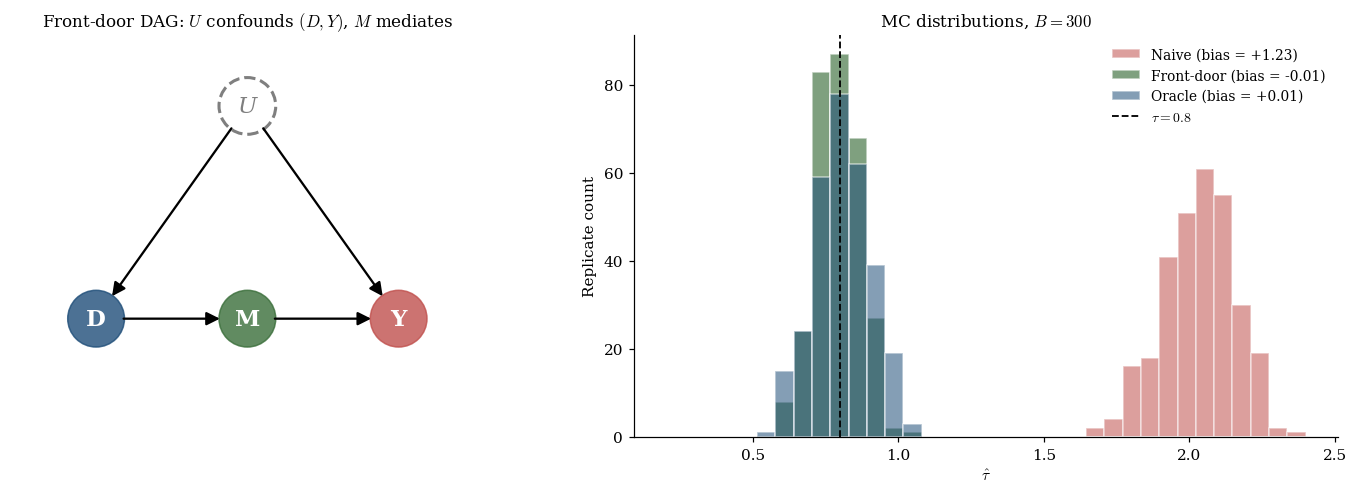
When unobserved confounders prevent back-door adjustment and no instrument is available, the front-door criterion (Pearl 1995) provides identification via a mediator on the pathway.
Conditions: (a) all paths go through — no direct effect; (b) is unconfounded — no back-door from to ; (c) the back-door from to is blocked by . The canonical example is smoking → tar → cancer with unobserved genetic confounder.
The front-door criterion. Under (a)–(c), Pearl’s do-calculus gives
For binary with continuous and , the ATE is
The notebook implements this via a single OLS fit of on , computes for each unit, and takes a difference of arm-means; the result tracks the oracle estimator (which knows ) to within Monte Carlo noise while the naive contrast is biased upward by the confounding through .
Generalizations. Front-door and back-door are two criteria within Pearl’s do-calculus, the complete identification framework. Shpitser–Pearl (2006) gives a completeness theorem: an effect is identifiable iff do-calculus derives its expression. For longitudinal time-varying treatment with time-varying confounding, Robins’s g-methods generalize the back-door criterion — the g-formula, marginal structural models, structural nested models. Hernán & Robins (2020) is the standard reference.
§11 Heterogeneous treatment effects
§§4–10 targeted scalar estimands. CATE is the function-valued target. Under ignorability and positivity, . CATE is the substrate for individualized decisions.
Meta-learners. Künzel et al. (2019) taxonomy:
- S-learner. Single ; CATE = . Biased toward zero when regularization shrinks the coefficient.
- T-learner. Two regressions , separately. Inefficient under arm imbalance but unbiased toward zero.
- X-learner (Künzel et al. 2019). Imputed pseudo-effects combined via propensity weights — better at extrapolating across imbalanced arms.
- R-learner (Nie & Wager 2021). Partial out and ; minimize the Robinson residual loss. Neyman-orthogonal at the population level.
- DR-learner (Kennedy 2020). Cross-fit AIPW pseudo-outcomes — by construction — then regress on . Inherits the doubly-robust property pointwise. Modern default.
Causal forests. Wager & Athey (2018), Athey, Tibshirani, and Wager (2019) adapt random forests to CATE with (i) a treatment-effect splitting criterion (maximize within-leaf treatment-effect variance) and (ii) honest splitting — fit the tree on one half, estimate within-leaf effects on the other. Honesty enables pointwise asymptotic normality via the infinitesimal jackknife.
Why CATE matters. The optimal treatment rule depends on the CATE function pointwise. Policy value quantifies expected outcome under the rule. Policy learning (Kitagawa & Tetenov 2018; Athey & Wager 2021), heterogeneity tests (Athey & Imbens 2016; Chernozhukov et al. 2018), and subgroup analysis via generalized random forests are all built on CATE estimates.
§12 Sensitivity analysis
The unmeasured-confounding problem. The bias of any back-door-adjusted estimator under unobserved scales as , where is the partial effect of on . Either piece zero ⇒ zero bias. Sensitivity analysis asks: how large would the unobserved piece need to be in order to nullify the observed effect?
Rosenbaum bounds. Parameterize the maximum within-matched-pair odds-ratio gap an unobserved can induce by . The tipping-point is the smallest value at which the worst-case p-value crosses 0.05. Published medical studies typically report tipping points in . Rosenbaum (1987, 2002) is the comprehensive reference.
The E-value (and Cinelli–Hazlett robustness value). For an observed risk ratio , VanderWeele and Ding (2017) define
For , replace by . Interpretation: the minimum confounding strength (RR scale, with both treatment and outcome) needed to nullify the effect. For continuous outcomes, approximate via for standardized effect . Computable at point and at CI bound; the latter is more conservative. VanderWeele–Ding benchmarks: 1.5 modest, 3 moderate, 5+ strong.
For a linear regression with unobserved , the Cinelli–Hazlett (2020) Robustness Value is
where . is the value at which produces bias . The conservative pushes the CI to include zero. Both diagnostics report on different scales and should be reported together — the E-value lives on the risk-ratio scale, the RV lives on the partial- scale.
Practical reporting. Three recommendations (VanderWeele & Ding 2017; Cinelli & Hazlett 2020): (1) always report some sensitivity diagnostic for observational studies — the E-value is the cheapest; (2) pair point estimates with CI-based sensitivity on multiple scales (E-value and RV); (3) calibrate against domain benchmarks. The caveat: sensitivity analysis quantifies robustness to unmeasured confounding, not to misspecification among observed covariates — the §6 doubly-robust property addresses the latter.
§13 Worked example: end-to-end on the Robinson DGP
The full pipeline threads §§4–8 estimators through one estimation routine. The DGP is the canonical Robinson DGP from §1.4: , , , , .
Nuisance fits are lasso CV (logistic with L1 penalty for the propensity, lasso CV per arm for the outcome) and a kernel-smoother RF proxy (the in-browser substitute for the notebook’s full RandomForestRegressor). The forest plot shows IPW (Hájek), OR (g-comp), AIPW, DML-lasso, and DML-RF-proxy point estimates with 95% Wald CIs; the lower panel overlays the Monte Carlo distributions across replicates.
Remark (Cross-check against doubleml).
The Python notebook includes an optional cross-check against the doubleml package on a single sample. Hand-rolled DML-lasso returns with ; doubleml.DoubleMLPLR returns with . The two agree to within Monte Carlo noise, as expected — the hand-rolled implementation gives us full control over the cross-fitting harness and the score evaluation, while doubleml is the reference for production work.
Coverage table. Across replicates at on the canonical Robinson DGP, the notebook reports the following: IPW (Hájek) achieves 0.97 coverage with mean SE 0.10; AIPW achieves 0.89 with mean SE 0.07; DML-lasso achieves 0.95 with mean SE 0.10; DML-RF achieves 0.91 with mean SE 0.07. OR achieves 0.07 coverage because the naive plug-in SE ignores first-stage fitting noise — under-coverage of OR is expected and the §6 AIPW-based variance is the right alternative.
Sensitivity diagnostics on the AIPW estimate. On the single-sample AIPW point estimate at with , : E-value (point) = 2.96, E-value (CI lower) = 2.74, , . All four diagnostics agree that nullifying this effect would require an unmeasured confounder roughly as strong as a moderate epidemiological exposure-outcome pair (RR ≈ 3 on the risk-ratio scale, or partial of about 0.34 on both the treatment and the outcome residualized on observed covariates).
§14 Connections and limits
Rubin vs Pearl. Two traditions — potential outcomes (Neyman, Rubin) and DAGs (Wright, Pearl). For binary-treatment ATE, they give equivalent identification claims and estimators; they differ in what they make easy to express. The Rubin tradition makes unit-level claims and randomization-based design natural; the Pearl tradition makes structural claims and do-calculus natural. Modern applied work mixes both. The framework chosen for this topic is the potential-outcomes one because it gives the cleanest setup for the §§4–8 estimator zoo; the §10 front-door section pivots to the DAG framework because that is where it lives most naturally.
Longitudinal extensions. Time-varying treatment and time-varying confounding break the static back-door criterion: a covariate measured after an earlier treatment can be both a confounder for later treatment and a mediator for the earlier one. Robins’s g-methods generalize: the longitudinal g-formula, marginal structural models with longitudinal IPW, structural nested models with longitudinal OR. Hernán & Robins (2020) is the standard reference.
What causal inference cannot do. (a) The no-unmeasured-confounders ceiling: no procedure recovers from observational data alone when ignorability fails — sensitivity analysis (§12) bounds the magnitude of unobserved confounding required to overturn a finding but cannot identify itself. (b) Effects of non-manipulable “treatments” (race, gender, age) require careful specification of the manipulation regime — Holland (1986)‘s “no causation without manipulation” formulation is one stance; modern mediation analysis (VanderWeele 2015) is another. (c) Extrapolation beyond observed treatment support requires parametric assumptions outside the framework — IPW, OR, AIPW are silent on what happens for values with on the support boundary.
Forward pointers. Mediation analysis (VanderWeele 2015) extends the potential-outcomes framework to decompose total effects into direct and indirect components. Dynamic treatment regimes (Murphy 2003; Chakraborty & Moodie 2013) extend longitudinally and connect to offline reinforcement learning (Levine et al. 2020) and off-policy evaluation (Thomas & Brunskill 2016). Causal discovery (PC, FCI, NOTEARS — Zheng et al. 2018) tries to learn the DAG from data when it is not known a priori. Online causal inference and bandits (Athey et al. 2022; Hadad et al. 2021) extend the framework to adaptive data collection.
The §§3–8 framework is a building block. Future estimators built on top of sequence models, learned policies, and adaptive data will inherit the AIPW score, the doubly-robust property, Neyman orthogonality, and cross-fitting as substrate — the same way every modern model-selection rule inherits training-error-plus-capacity-penalty from structural risk minimization and every modern generalization bound inherits empirical-process / uniform-convergence machinery from formalStatistics: Empirical Processes .
Connections
- PAC-Bayes bounds and the §8.2 Neyman-orthogonality argument share the same Taylor-expansion-around-truth machinery: the first-order term vanishes at the true parameter / true nuisance, leaving a second-order remainder that the Donsker-class structure tames. DML inherits the $\sqrt{n}$ rate from a Neyman-orthogonal score the way PAC-Bayes inherits the dimension-free bound from its orthogonality between the posterior and the prior. pac-bayes-bounds
- SRM picks a single hypothesis class from a nested family; DML picks a single ATE estimator from a class of cross-fitted nuisance fits. Both rely on the rate of nuisance estimation falling below a critical threshold ($o_P(n^{-1/4})$ for DML, $o_P(n^{-1/2})$ for SRM consistency); both depend on uniform-convergence machinery underwriting the per-instance plug-in argument. SRM is model selection in supervised learning; DML is model selection at the nuisance-estimation step of causal inference. structural-risk-minimization
- Lasso is the workhorse nuisance estimator in §§8, 13 of this topic; the restricted-eigenvalue + sparsity rate that delivers $o_P(n^{-1/4})$ consistency comes directly from the high-dimensional-regression topic. The §8.2 Neyman-orthogonality argument requires $\|\hat\eta - \eta_0\|_2 = o_P(n^{-1/4})$, which lasso achieves under sparsity (Bickel–Ritov–Tsybakov 2009) covered in that topic. high-dimensional-regression
- The plug-in sandwich variance for IPW (§4.3), the AIPW EIF variance (§6.4), and the DML $\sqrt{n}$-asymptotic-normality result (§8.4) all rely on standard concentration inequalities (Hoeffding, Bernstein, McDiarmid) for the empirical-process step. The §12 Rosenbaum bound is itself a closed-form Bernoulli concentration result expressed in tipping-point form. concentration-inequalities
References & Further Reading
- paper Estimation of the Parameters of a Single Equation in a Complete System of Stochastic Equations — Anderson & Rubin (1949) The original Anderson–Rubin weak-IV-robust test, inverted to produce confidence sets that remain valid when the first-stage F-statistic is small.
- paper Weak Instruments in Instrumental Variables Regression: Theory and Practice — Andrews, Stock & Sun (2019) Modern survey of weak-IV diagnostics and inference, including the $F > 23.1$ tightening of the Staiger–Stock rule of thumb (Annu. Rev. Econ. 11).
- paper Recursive Partitioning for Heterogeneous Causal Effects — Athey & Imbens (2016) Heterogeneity tests for CATE via causal trees (PNAS 113.27).
- paper Generalized Random Forests — Athey, Tibshirani & Wager (2019) The honest-splitting + local-moment machinery behind causal forests (Ann. Stat. 47.2).
- paper Policy Learning with Observational Data — Athey & Wager (2021) Optimal treatment-rule estimation built on the DR-score (Econometrica 89.1).
- paper Contextual Bandits in a Survey Experiment on Charitable Giving — Athey, Byambadalai, Hadad, Krishnamurthy, Leung & Williams (2022) Adaptive policy learning on a real survey experiment (arXiv).
- paper Doubly Robust Estimation in Missing Data and Causal Inference Models — Bang & Robins (2005) The modern crisp formulation of AIPW that we adopt in §6 (Biometrics 61.4).
- book Statistical Methods for Dynamic Treatment Regimes — Chakraborty & Moodie (2013) Reference for longitudinal extensions (§14.2) and dynamic-treatment-regime estimation (Springer).
- paper Double/Debiased Machine Learning for Treatment and Structural Parameters — Chernozhukov, Chetverikov, Demirer, Duflo, Hansen, Newey & Robins (2018) The DML paper; the §8.4 theorem we present is Theorem 3.1 (Econometrics Journal 21.1).
- paper Making Sense of Sensitivity: Extending Omitted Variable Bias — Cinelli & Hazlett (2020) Robustness Value $RV_q$ and the associated benchmarking framework used in §12.3 (JRSS-B 82.1).
- paper Plausibly Exogenous — Conley, Hansen & Rossi (2012) Sensitivity analysis for partial-exclusion-violation in IV (Rev. Econ. Stat. 94.1).
- paper Smoking and Lung Cancer: Recent Evidence and a Discussion of Some Questions — Cornfield, Haenszel, Hammond, Lilienfeld, Shimkin & Wynder (1959) The Cornfield-condition argument — the historical antecedent of the E-value (J. Natl. Cancer Inst. 22.1).
- paper Dealing with Limited Overlap in Estimation of Average Treatment Effects — Crump, Hotz, Imbens & Mitnik (2009) Optimal trimming for IPW under near-positivity violation (Biometrika 96.1).
- paper Deep Neural Networks for Estimation and Inference — Farrell, Liang & Misra (2021) Neural-net rate conditions sufficient for DML (Econometrica 89.1).
- paper Confidence Intervals for Policy Evaluation in Adaptive Experiments — Hadad, Hirshberg, Zhan, Wager & Athey (2021) Inference for adaptively-collected experimental data (PNAS 118.15).
- paper On the Role of the Propensity Score in Efficient Semiparametric Estimation of Average Treatment Effects — Hahn (1998) The Hahn efficiency bound for the ATE (Econometrica 66.2).
- book Causal Inference: What If — Hernán & Robins (2020) Standard reference; freely available online (Chapman & Hall/CRC).
- paper Efficient Estimation of Average Treatment Effects Using the Estimated Propensity Score — Hirano, Imbens & Ridder (2003) The estimated-propensity efficiency result we cite in §4.3 (Econometrica 71.4).
- paper Statistics and Causal Inference — Holland (1986) Names the fundamental problem of causal inference (JASA 81.396).
- paper A Generalization of Sampling Without Replacement from a Finite Universe — Horvitz & Thompson (1952) The Horvitz–Thompson IPW estimator (JASA 47.260).
- paper Sensitivity to Exogeneity Assumptions in Program Evaluation — Imbens (2003) Sensitivity analysis for treatment-effect estimators (AER 93.2).
- paper Identification and Estimation of Local Average Treatment Effects — Imbens & Angrist (1994) The LATE theorem under monotonicity (Econometrica 62.2).
- paper Optimal Doubly Robust Estimation of Heterogeneous Causal Effects — Kennedy (2020) The DR-learner construction we use in §11.2 (arXiv).
- paper Who Should Be Treated? Empirical Welfare Maximization Methods for Treatment Choice — Kitagawa & Tetenov (2018) Optimal-policy estimation in finite-sample (Econometrica 86.2).
- paper Metalearners for Estimating Heterogeneous Treatment Effects Using Machine Learning — Künzel, Sekhon, Bickel & Yu (2019) The S/T/X-learner taxonomy used in §11.2 (PNAS 116.10).
- paper Offline Reinforcement Learning: Tutorial, Review, and Perspectives on Open Problems — Levine, Kumar, Tucker & Fu (2020) Forward pointer to off-policy RL in §14.4 (arXiv).
- paper Robust Metrics and Sensitivity Analyses for Meta-Analyses of Heterogeneous Effects — Mathur & VanderWeele (2020) E-value applications in meta-analysis (Epidemiology 31.3).
- paper A Conditional Likelihood Ratio Test for Structural Models — Moreira (2003) Conditional likelihood-ratio test for weak IV (Econometrica 71.4).
- paper Optimal Dynamic Treatment Regimes — Murphy (2003) Foundational paper on dynamic treatment regimes (JRSS-B 65.2).
- paper On the Application of Probability Theory to Agricultural Experiments — Neyman (1990) 1923 original, translated 1990; the first formal potential-outcomes framework (Statistical Science 5.4).
- paper Quasi-Oracle Estimation of Heterogeneous Treatment Effects — Nie & Wager (2021) The R-learner construction with Neyman-orthogonal residual loss (Biometrika 108.2).
- paper Causal Diagrams for Empirical Research — Pearl (1995) Front-door criterion + do-calculus (Biometrika 82.4).
- book Causality: Models, Reasoning, and Inference — Pearl (2009) Comprehensive reference for the graphical / do-calculus framework (Cambridge University Press, 2nd ed.).
- paper A New Approach to Causal Inference in Mortality Studies with a Sustained Exposure Period — Robins (1986) The g-computation algorithm (Math. Modelling 7).
- paper Estimation of Regression Coefficients When Some Regressors Are Not Always Observed — Robins, Rotnitzky & Zhao (1994) The original AIPW score in missing-data form (JASA 89.427).
- paper Root-N-Consistent Semiparametric Regression — Robinson (1988) The partial-linear model that threads the worked example (Econometrica 56.4).
- paper Sensitivity Analysis for Certain Permutation Inferences in Matched Observational Studies — Rosenbaum (1987) The Rosenbaum-bound construction (Biometrika 74.1).
- book Observational Studies — Rosenbaum (2002) Comprehensive reference for sensitivity analysis (Springer, 2nd ed.).
- paper The Central Role of the Propensity Score in Observational Studies for Causal Effects — Rosenbaum & Rubin (1983) The propensity-score balancing-score theorem (Biometrika 70.1).
- paper Estimating Causal Effects of Treatments in Randomized and Nonrandomized Studies — Rubin (1974) The Rubin Causal Model (J. Educ. Psychol. 66.5).
- paper Discussion of 'Randomization Analysis of Experimental Data: The Fisher Randomization Test' by D. Basu — Rubin (1980) SUTVA formulation (JASA 75.371).
- paper Identification of Joint Interventional Distributions in Recursive Semi-Markovian Causal Models — Shpitser & Pearl (2006) Completeness theorem for do-calculus (AAAI-06).
- paper Instrumental Variables Regression with Weak Instruments — Staiger & Stock (1997) The original $F > 10$ rule of thumb (Econometrica 65.3).
- paper The Calculus of M-Estimation — Stefanski & Boos (2002) M-estimator sandwich variance framework underwriting §§4.3, 6.4 (American Statistician 56.1).
- book Testing for Weak Instruments in Linear IV Regression — Stock & Yogo (2005) Stock–Yogo critical-value tables for weak-IV inference (Cambridge University Press).
- paper Data-Efficient Off-Policy Policy Evaluation for Reinforcement Learning — Thomas & Brunskill (2016) Off-policy evaluation that imports IPW/AIPW into RL (ICML).
- book Targeted Learning: Causal Inference for Observational and Experimental Data — van der Laan & Rose (2011) Comprehensive TMLE reference (Springer).
- paper Targeted Maximum Likelihood Learning — van der Laan & Rubin (2006) The original TMLE paper (Int. J. Biostat. 2.1).
- book Explanation in Causal Inference: Methods for Mediation and Interaction — VanderWeele (2015) Mediation analysis (Oxford University Press).
- paper Sensitivity Analysis in Observational Research: Introducing the E-Value — VanderWeele & Ding (2017) The E-value, with VanderWeele–Ding moderate/strong benchmarks 1.5 / 3 / 5+ (Ann. Intern. Med. 167.4).
- paper Estimation and Inference of Heterogeneous Treatment Effects Using Random Forests — Wager & Athey (2018) Causal forests with pointwise asymptotic normality (JASA 113.523).
- book The Tariff on Animal and Vegetable Oils — Wright (1928) Appendix B introduces the original IV identification argument (Macmillan).
- paper The Method of Path Coefficients — Wright (1934) The path-diagram precursor to modern DAGs (Ann. Math. Stat. 5.3).
- paper DAGs with NO TEARS: Continuous Optimization for Structure Learning — Zheng, Aragam, Ravikumar & Xing (2018) Modern continuous-optimization approach to causal discovery (NeurIPS 31).