Kernel Regression
Nonparametric estimation of conditional means via the Nadaraya–Watson estimator — bias-variance decomposition with the design-density correction, AMISE-optimal bandwidth selection, the curse of dimensionality at higher d, and the local-linear fix for boundary bias.
1. From parametric to nonparametric: the local-averaging idea
This section motivates kernel regression by showing that parametric assumptions fail badly when the shape of is genuinely unknown. We introduce the synthetic toy that runs through the topic, walk through the local-averaging intuition geometrically, and motivate why a smooth kernel weight is preferable to a hard-edged box. No algebra yet — that arrives with the Nadaraya–Watson estimator in §2.
1.1 The regression problem when shape is unknown
We observe iid pairs for , drawn from a joint distribution with marginal density for and conditional mean function
The regression problem is to estimate from the sample. Parametric regression assumes lives in some finite-dimensional family — affine in , polynomial of fixed degree, additive across coordinates, and so on. If the assumption holds, parametric estimators are efficient: they converge at the parametric rate , and standard inference machinery just works. If it fails, the estimator is biased in a way that doesn’t go away with more data; we’d be efficiently converging to the wrong answer.
The whole topic runs on the toy
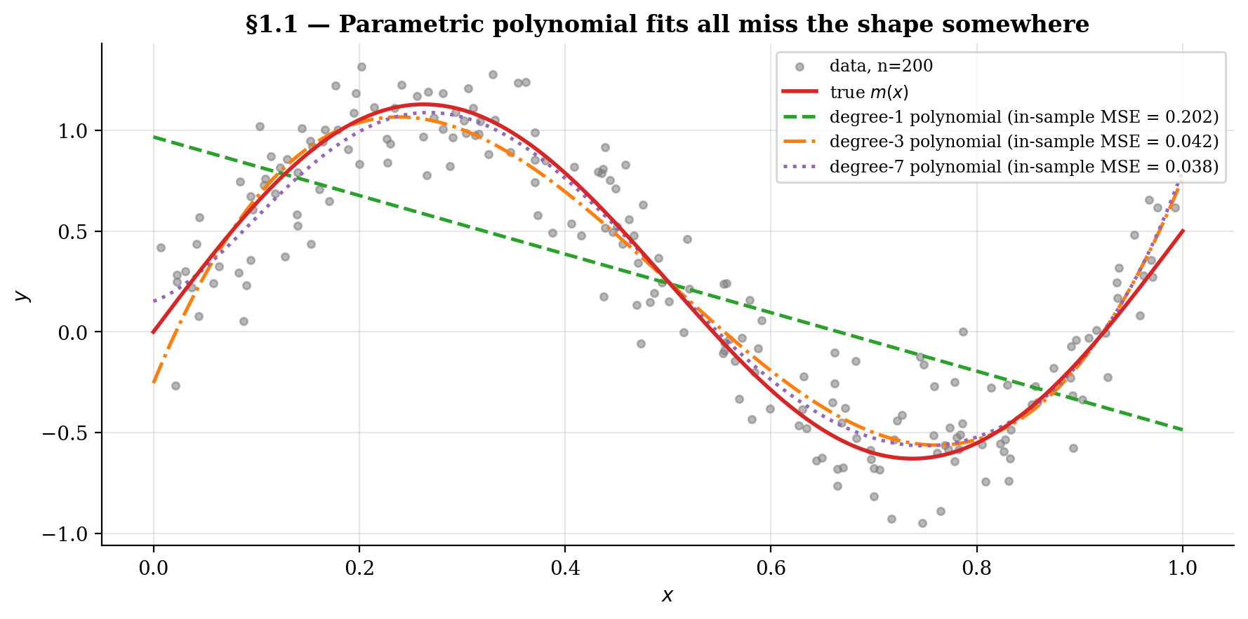
with . The figure below scatters the data and overlays three polynomial fits — degree-1, degree-3, degree-7. Low degrees underfit the sinusoid, the high-degree fit over-oscillates at the boundaries (a preview of the Runge phenomenon and the boundary-bias story we revisit in §8). None of them gets the shape right uniformly.
1.2 What “local averaging” means geometrically
If we don’t know the shape of globally, we can still use a weak local assumption: is continuous (or smoother), so observations whose sits close to a target should carry values close to on average. The basic idea behind every kernel-smoothing method falls out of this — to estimate , average the values for which is “near” . The noise mostly cancels and what’s left is approximately .
The simplest “near” predicate is the box: include in the average when for some half-width . This gives the box-average estimator.
Example 1 (Box-average estimator).
For a target point and bandwidth , the box-average estimator of is
where is the indicator function (1 when the condition holds, 0 otherwise). The estimator averages the values whose falls inside .
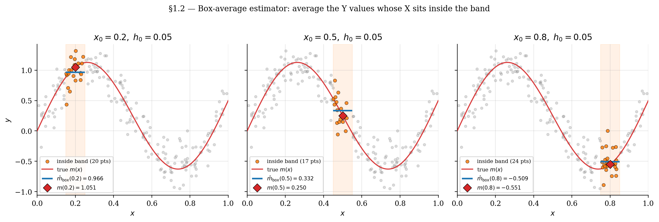
The viz below lets you drag the target along the support and adjust the band half-width . The highlighted points (orange) are the in-band observations whose values get averaged; the blue segment marks and the red ring marks the true . When the band is small enough that is nearly constant inside it but wide enough to contain enough points, the average lands close to .
Drag x₀ along the support; the highlighted points (orange) are the in-band observations whose Y values get averaged. The blue segment shows that local box average; the red ring marks the true m(x₀). Shrink h₀ to see variance dominate (few points → noisy average); grow h₀ to see bias dominate (many points but they smear m's curvature).
This is the core idea. The next subsection points out where it falls short and what to do about it.
1.3 From boxes to kernels: why we don’t just bin
The box-average estimator from §1.2 has two problems that motivate the kernel approach.
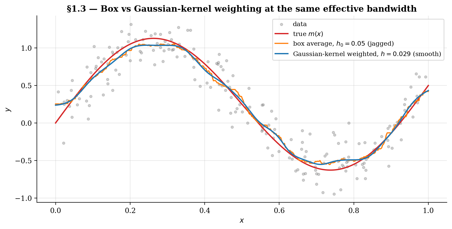
Problem 1: Discontinuity. As the target slides smoothly across the support, individual observations enter and leave the band abruptly. Each entry or exit shifts the local average by a discrete amount. The resulting curve is visibly jagged even though the underlying is smooth — we’ve imposed our own discontinuity onto the estimator through the indicator function.
Problem 2: Information loss at the band edge. Within the band, the box treats every observation as equally relevant. A point at contributes the same weight as one at , even though the latter is far more informative about when is continuous. The “closer is more informative” intuition we used to motivate local averaging is precisely what the box discards.
Both problems have the same fix. Replace the indicator with a smooth, decreasing weight function — a kernel. The kernel returns a high value when is close to , a low value when is far, and varies continuously in between. The estimator inherits the kernel’s smoothness in (problem 1 fixed) and observations are weighted by proximity rather than treated as equivalent (problem 2 fixed).
This sets up §2, where we make the kernel-weight idea precise — the moment conditions a kernel must satisfy, the resulting Nadaraya–Watson formula, and its closed-form expression as a degree-zero local polynomial regression.
2. The Nadaraya–Watson estimator
This section formalizes the kernel-weighting idea from §1.3. We define the kernel function via four standard moment conditions, derive the Nadaraya–Watson estimator two ways — as a plug-in conditional-mean estimator (ratio of joint and marginal density estimates) and as a locally-weighted least-squares solution — and show the two derivations agree. The locally-weighted-OLS view is what makes §8’s local-linear extension natural.
2.1 Kernel functions and their four moment conditions
Definition 1 (Kernel).
A (one-dimensional, second-order) kernel is a function satisfying:
- Nonnegativity and symmetry: for all , and .
- Normalization: .
- Zero first moment: . (This follows from symmetry but is worth stating separately — it’s what makes the leading-order bias term in §3 quadratic in rather than linear.)
- Finite second moment: .
A fifth quantity used repeatedly is the kernel-second-moment integral , which controls the variance term in the AMISE.
The rescaled kernel is
so that for any bandwidth . We write the NW estimator using either or the explicit form depending on which is cleaner in context.
Five kernels appear throughout the topic — Gaussian, Epanechnikov, box (uniform), triangular, quartic. We compare them systematically in §7. The figure below introduces the cast and tabulates and for each.
![The five standard kernels (Gaussian, Epanechnikov, box, triangular, quartic) overlaid on u in [-3, 3].](/images/topics/kernel-regression/04_standard_kernels.png)
2.2 The NW formula as a closed-form weighted average
Definition 2 (Nadaraya–Watson estimator).
The Nadaraya (1964) / Watson (1964) estimator of is
The cleanest derivation is as a plug-in estimator. The conditional mean factors as
Replace the unknown densities by their kernel density estimates:
and integrate against . Using the kernel’s first-moment condition — implies , and a change of variables gives — the integral collapses to the ratio above. NW is exactly the plug-in version of where the joint density is replaced by its KDE.
This is why kernel regression sits where it does in the curriculum: it’s the conditional-mean sequel to formalStatistics: Kernel Density Estimation — same kernel machinery, applied one level up.
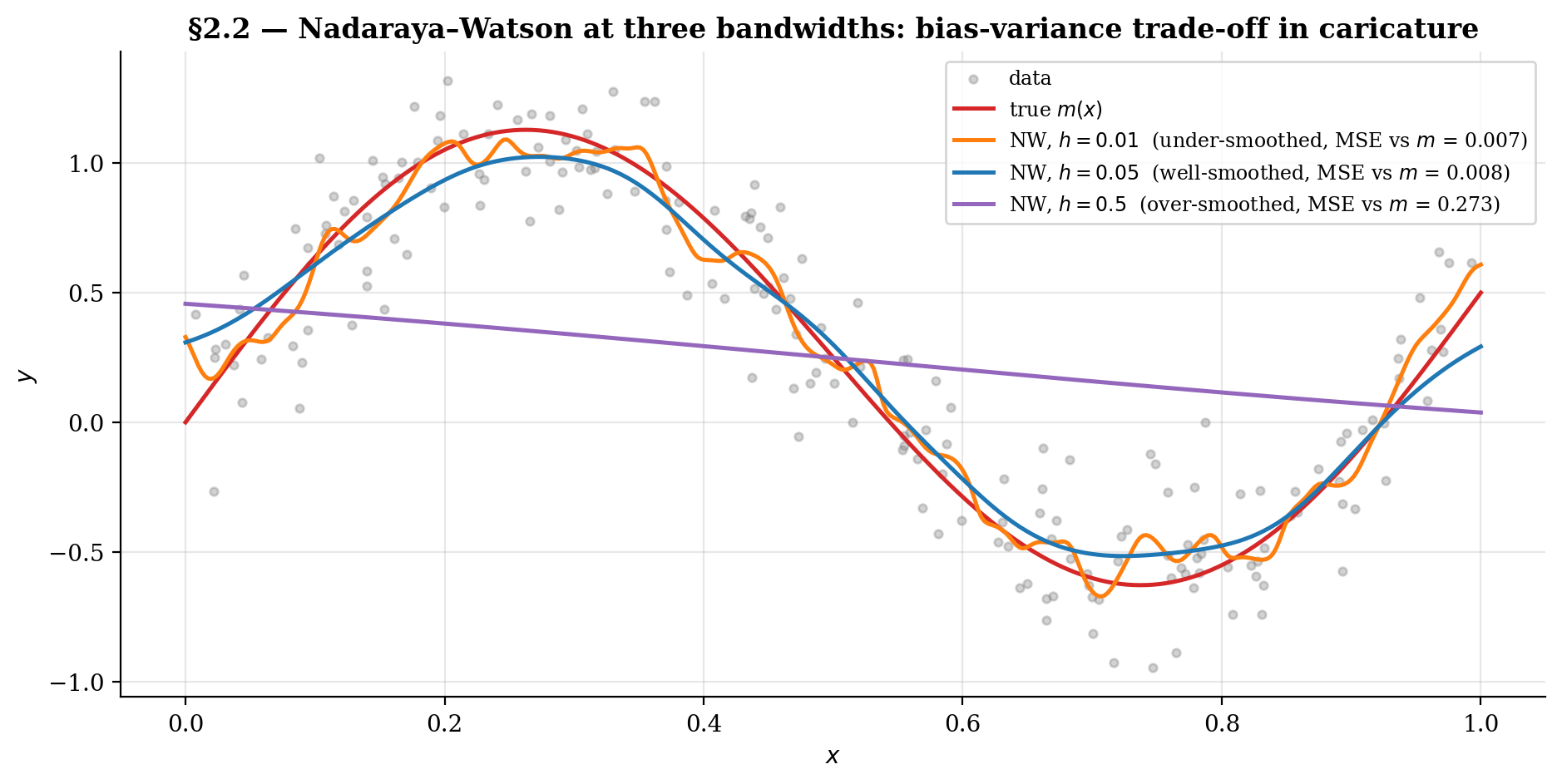
The viz below shows NW at three bandwidth regimes — under-smoothed, well-smoothed, over-smoothed — on the §1 toy. The pattern is the bias-variance trade-off in caricature, formalized asymptotically in §3–§4. Drag the bandwidth slider across log-space; click the “snap to ” button to jump to the AMISE-optimal value (we derive in §4.4).
Drag h smoothly across log-space (0.005 to 0.5). Watch the bias-variance trade-off in caricature: under-smoothing chases noise, over-smoothing flattens the sinusoid. The h* button snaps to the AMISE-optimal bandwidth for the current n; at n = 200 that's h* ≈ 0.037, where grid-MSE bottoms out near 0.008.
2.3 NW as degree-zero local polynomial regression
The same estimator falls out of a different optimization problem. Fix a target and consider the locally-weighted least-squares problem
We’re fitting a single scalar — a constant approximation to — with each observation weighted by its kernel-proximity to .
Lemma 1 (NW = degree-zero local polynomial regression).
The NW estimator equals the kernel-weighted least-squares minimizer above.
Proof.
Take the derivative of the objective with respect to and set it to zero:
The second equality is the definition of NW from Definition 2.
∎So NW is exactly degree-zero local polynomial regression: at each , fit the best constant approximation to over a kernel-weighted neighborhood.
This reframing pays off twice. It motivates §8’s local-linear regression — instead of a constant, fit a line over the same kernel neighborhood, which corrects the boundary-bias problem we’ll see in §3.4. And it lets us re-use any weighted-least-squares solver to compute NW, giving us a check on the direct implementation.
In NumPy, the vectorized form is a single matrix multiply per query grid:
def nadaraya_watson(X, Y, x_eval, h, K=K_gaussian):
    """Vectorized NW: returns hat m_h(x) for each entry of x_eval."""
    U = (X[None, :] - x_eval[:, None]) / h          # shape (|x_eval|, n)
    W = K(U) / h                                    # rescaled kernel weights
    return (W @ Y) / W.sum(axis=1)                  # weighted average per row
A numerical sanity check: pick a single target , compute via the direct NW formula, and compute it again via the explicit WLS solution with design matrix (a column of ones) and weight matrix . Verification: NW direct , WLS , gap — agreement to numerical precision.
3. Pointwise bias at an interior point
This section derives the asymptotic bias of NW at an interior point of the support of . The argument has three substeps — Taylor expansion of the joint density estimate, change of variables to kernel-scaled coordinates, and a ratio expansion that combines the two — followed by a boundary preview that motivates §8’s local-linear fix.
Theorem 1 (Pointwise bias of NW (interior)).
Let be an interior point of the support of with and . As and ,
The first term is the curvature bias — present in any kernel-based estimator, including KDE for density estimation. The second term is the design-density correction — unique to regression. It vanishes when is uniform (the §1 toy), but in general the asymmetry of the design density tilts the local average toward the more-densely-sampled side.
We work through the proof in three substeps, then discuss the two terms separately.
3.1 The Taylor expansion of around
Write the NW estimator as a ratio. Define
so that , where is the kernel density estimate of . The strategy is to expand and to second order in , then combine them via a ratio expansion.
Because the are iid:
For , use the tower property to integrate out first:
where . Both expectations are integrals against centered at . The next move turns these integrals into closed-form polynomials in .
3.2 Change of variables to scaled coordinates
Substitute , so and . The integrals become
The factor inside exactly cancels the from the , leaving clean integrals against the unscaled kernel . Now Taylor-expand both integrands around (i.e., around ) to second order in :
By the product rule applied to :
Integrate term by term against and apply the four kernel moment conditions from Definition 1: keeps the constant term, kills the linear term, and scales the quadratic term. The result:
This is the technical heart of the proof. Taylor expansion plus the kernel moment conditions reduce a complicated integral to a polynomial in whose leading correction is quadratic — that’s where the rate comes from, and why the zero-first-moment condition is so important.
3.3 The design-density correction
Take the ratio. The exact bias of involves , which doesn’t factor cleanly. The standard move — justified by KDE consistency in probability (a foundational result from formalStatistics: Kernel Density Estimation ) plus uniform integrability — is to take the leading-order approximation
Plug in §3.2’s expansions. The constant term in cancels exactly with from the second numerator term, leaving
Substitute the formula for from §3.2:
The terms cancel. Divide by to recover the bias formula stated in Theorem 1.
The two terms have different physical interpretations.
Curvature bias ( term). The kernel-weighted average of a curved function is biased toward the side the function curves toward. At a local maximum (), the average pulls down; at a local minimum (), it pulls up. This is universal — it appears in KDE, in NW, and in any kernel-smoothing operation.
Design-density correction ( term). When is non-uniform, the kernel neighborhood around contains more values on the side where is larger. The local average is pulled toward -values from that side. The sign is determined by the product : positive correlation pushes above , negative pushes below. The correction vanishes when is uniform and grows where varies steeply.
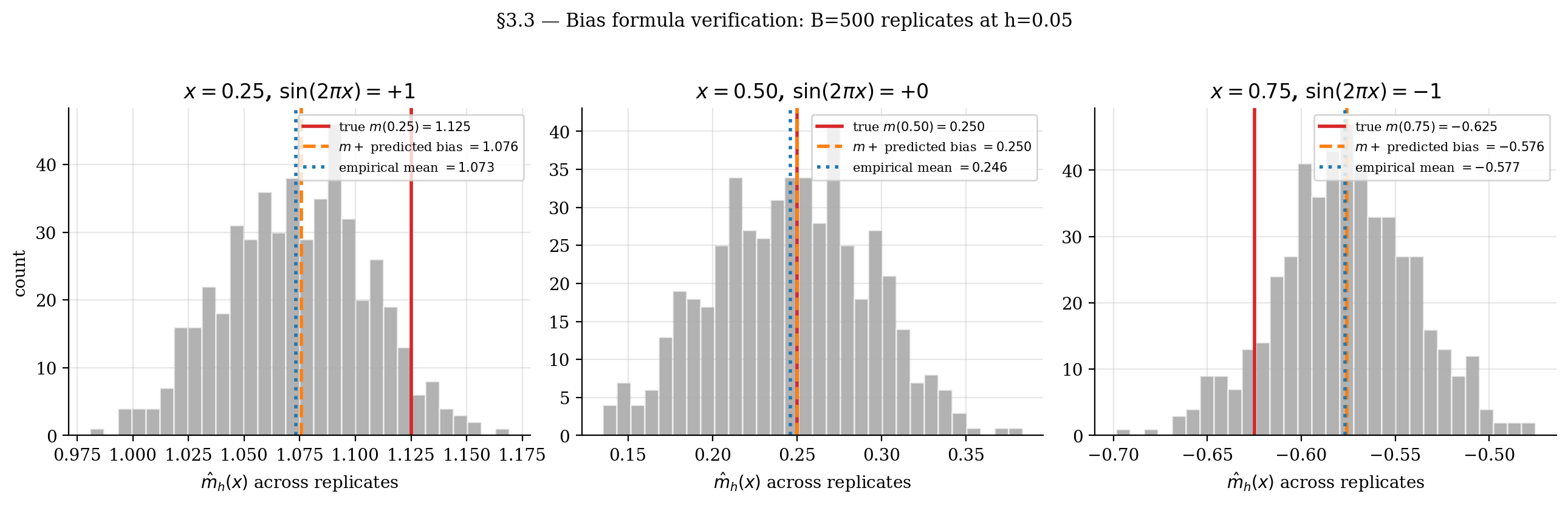
We verify the formula numerically on the §1 toy. With , on the interior, so the design correction drops out and the prediction collapses to
using and . At , where respectively, we predict bias at .
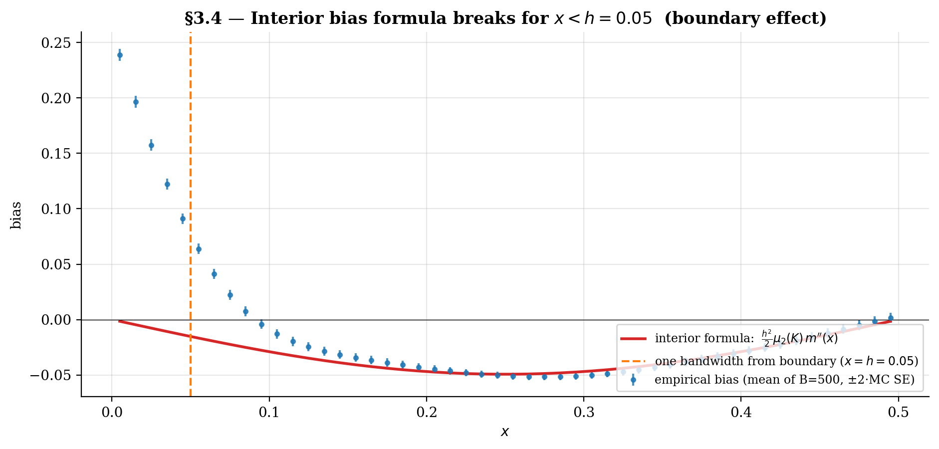
3.4 Preview: why the boundary breaks this
The expansion in §3.1–3.3 assumed is an interior point of the support — far enough from the boundary that the kernel mass within one bandwidth is fully contained in the support of . Concretely: over the relevant range, , and so on.
At a boundary point — for the §1 toy this means within one bandwidth of or , since — half of the kernel mass falls outside the support. The effective kernel is one-sided. Two of the four moment conditions break:
- The normalization becomes (for symmetric centered at the boundary).
- The zero first moment becomes .
The linear-in- term in the Taylor expansion of §3.2 no longer vanishes. The bias becomes instead of — an order worse than at the interior. This is the boundary bias problem for the Nadaraya–Watson estimator.
We revisit this in §8 with the local-linear regression fix that restores behavior all the way to the boundary.
4. Pointwise variance and the AMISE
We complete the bias-variance decomposition by computing the pointwise variance of , combining it with §3’s bias to form the asymptotic mean integrated squared error (AMISE), deriving the optimal bandwidth , and stating asymptotic normality.
Theorem 2 (Pointwise variance of NW).
Under the conditions of Theorem 1 plus ,
where from Definition 1.
4.1 The kernel-second-moment integral
Repeat the §3 setup: . To leading order,
Write . The summands are iid, so
Compute the second moment of the summand by conditioning on . Decompose
The cross term has zero conditional mean (since ); the third term contributes and is dominated by the variance scale. The leading contribution is
Change variables . The factor combined with produces a in front:
where the corrections to and get absorbed into the remainder. Combining with the prefactor gives the variance formula in Theorem 2. The scaling is the same one that makes KDE variance scale as — the “kernel mass concentrated in an -wide window over data points” rate.
4.2 The conditional-variance factor
Three components in the variance formula, each with its own physical interpretation.
The factor is the noise-to-density ratio at . Higher conditional noise inflates the variance — local averaging produces a noisier estimate when underlying responses are noisier. Lower design density inflates the variance — fewer values within one bandwidth means less data to average over. The two factors are local: both can vary across , and their ratio captures the effective sample size near .
The kernel-dependent constant measures how much variance the kernel passes through. Smaller means tighter weight concentration and smaller estimator variance. Among kernels with , the Epanechnikov kernel minimizes — the §7 optimality result.
The rate ties the variance to the effective number of points within one bandwidth, roughly in . More data (larger ) or wider bandwidth (larger ) gives more averaging and lower variance — the “wider-is-less-variable” half of the bias-variance trade-off. This is what fights against the growth of squared bias as increases, producing the U-shaped AMISE curve we see next.
4.3 Combining bias-squared and variance into AMISE
The pointwise mean squared error decomposes as
where collects the bias coefficient from Theorem 1.
The asymptotic mean integrated squared error is the integral of MSE against the design density:
where and are problem-specific constants depending on the unknown , , and .
The two terms move in opposite directions in : squared bias grows as (wider bandwidth → more curvature-induced bias), variance shrinks as (wider bandwidth → more effective averaging). The U-curve has a unique minimum at the optimal bandwidth .
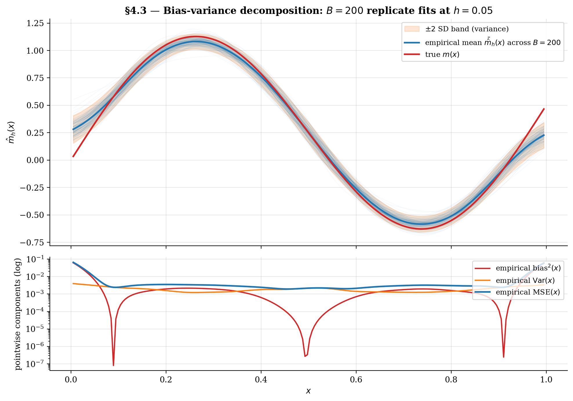
The viz below visualizes the decomposition empirically. Drag the bandwidth slider to see the replicate cloud spread (variance) and the empirical mean drift away from (bias). Crank up for tighter variance estimates.
At small h, the replicate cloud spreads wide (large variance) but the empirical mean tracks the true m(x) closely (small bias). Crank h up: the cloud collapses to a single smooth curve, but it visibly drifts away from m where the sinusoid curves. The integrated bias² and variance read-outs trade off through the AMISE U-curve in §4.4.
4.4 The optimal bandwidth and asymptotic normality
Differentiate AMISE in and set the derivative to zero:
Solving in :
The general -dimensional rate (proven in §6) is , with corresponding minimum AMISE at the rate .
This rate is slower than the parametric rate — the price for not assuming a parametric form for . In , kernel regression converges as . In it slows to . By it’s — barely better than the random-guess rate. This is the curse of dimensionality, formalized in §6.
For the §1 toy (, , , ):
The viz below shows the AMISE U-curve in closed form. Move the scrubber: as grows, the variance curve drops, shifts left, and AMISE() shrinks at the slow rate.
Two competing rates set the optimal bandwidth: bias² grows as h⁴ (slope +4 on log-log), variance falls as 1/(nh) (slope −1). Their sum bottoms out at h^* ∝ n^(-1/5). As n grows, the variance curve drops, h^* shifts left, and AMISE(h^*) shrinks at the slow nonparametric rate n^(-4/5) — much slower than the parametric n^(-1).
![AMISE U-curve over h in [0.005, 0.2] at n = 200, with empirical AMISE from B = 100 replicates per bandwidth and analytical curve overlaid.](/images/topics/kernel-regression/09_amise_ucurve.png)
Theorem 3 (Asymptotic normality of NW (Wand–Jones 1995, Theorem 5.4)).
Under the conditions of Theorems 1 and 2, plus and as ,
where from Theorem 1.
This gives the asymptotic confidence interval
The bias-correction term is usually estimated by plug-in or eliminated via undersmoothing (choose small enough that bias is dominated by variance, at the cost of slower convergence). The CI machinery is what links kernel regression to §9.4’s conformal-prediction interval construction.
5. Bandwidth selection in practice
The AMISE-optimal bandwidth from §4.4 depends on unknown functionals of , , and , so we can’t use it directly on real data. Three families of selectors estimate from observations:
- Reference-rule selectors (Silverman): substitute a parametric proxy for the unknowns. Fast, biased, no data adaptation.
- Plug-in selectors (Ruppert–Sheather–Wand DPI): estimate the unknowns from a pilot bandwidth, plug into the AMISE formula. Faster asymptotic convergence than CV but heavier to implement.
- Cross-validation selectors (LOO-CV, GCV): minimize an out-of-sample squared loss directly. Generalize cleanly to higher dimensions and don’t require pilot estimation.
We discuss Silverman in §5.1, plug-in conceptually in §5.2, and implement LOO-CV and GCV from scratch in §5.3–§5.4 using the smoother-matrix infrastructure . §5.5 compares all four on the §1 toy and assesses stability across replicate samples.
5.1 Silverman’s rule of thumb (and where it fails)
Silverman’s (1986) rule of thumb for KDE in is
where is a robust spread estimate of (the IQR/1.34 reduces sensitivity to outliers). The 1.06 constant comes from optimizing AMISE for KDE under a Gaussian-reference assumption on .
Three reasons the rule falls short for NW regression.
Wrong objective. Silverman is optimal for density estimation, not for conditional-mean estimation. The AMISE-optimal NW bandwidth depends on , , and — none of which the rule sees.
Gaussian-reference is overly smooth. Real densities and regression functions typically have more curvature than Gaussian, calling for smaller . The rule oversmooths in those cases.
No data adaptation. The bandwidth is fixed across , ignoring local variation in or .
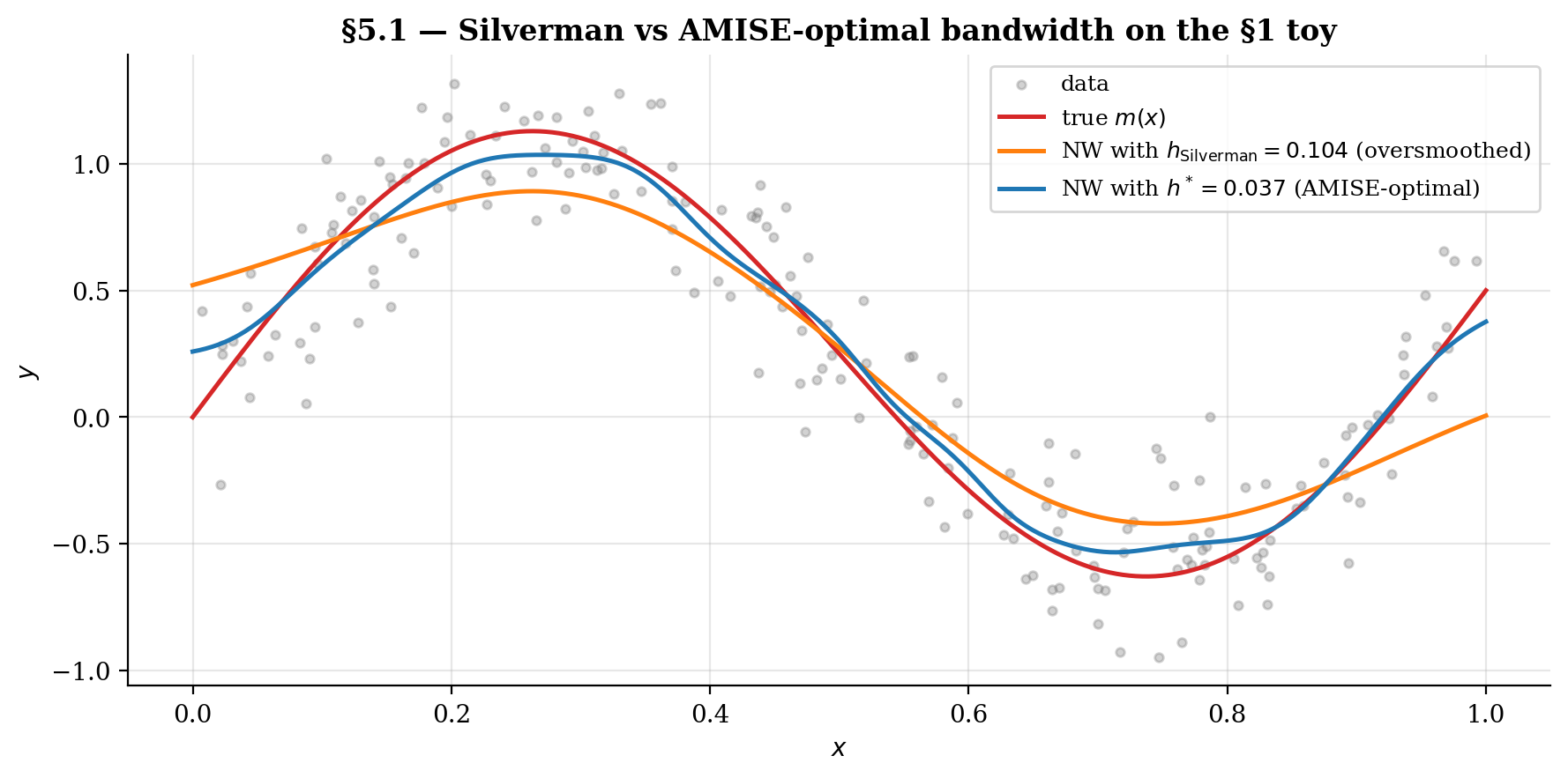
For the §1 toy (, ), Silverman gives . That’s about the analytical from §4.4 — a meaningful oversmoothing. Despite the limitations, Silverman remains useful as an order-of-magnitude reference and as a starting pilot bandwidth for plug-in estimators.
5.2 Plug-in selectors
The plug-in idea: substitute consistent estimates of the unknown functionals into the AMISE formula
The challenge is estimating — this requires estimating , a higher-order derivative that is itself harder to estimate than . The canonical solution is Ruppert–Sheather–Wand (1995) direct plug-in (DPI):
- Pick a pilot bandwidth (typically Silverman’s rule).
- Fit a degree-4 local polynomial at to estimate at each .
- Estimate from residuals at , and from a KDE at .
- Form and from the residual variance.
- Plug into the AMISE formula to get .
Plug-in selectors converge to at faster rates than CV ( for RSW vs for CV; see Härdle, Marron & Park 1992), but they require non-trivial implementation. The chicken-and-egg problem of pilot-bandwidth selection is well-studied (Ruppert 1997’s EBBS iterates the pilot to convergence).
For this topic we mention plug-in selectors conceptually and reference RSW; the full implementation is heavy enough to warrant a sister-topic extension. The remainder of §5 focuses on cross-validation selectors, which generalize more naturally to higher-dimensional settings and don’t require pilot estimation.
5.3 Leave-one-out cross-validation
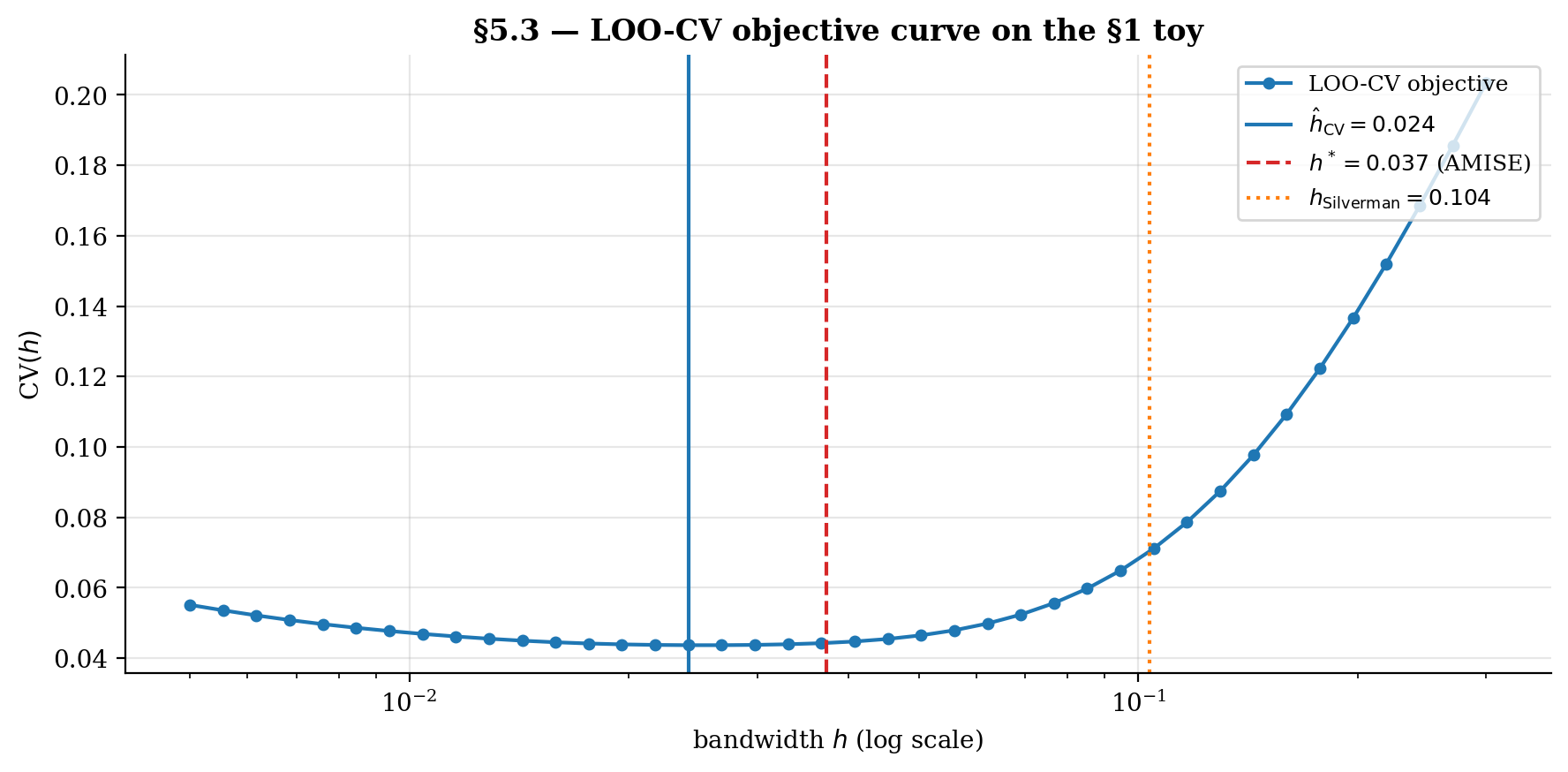
Cross-validation estimates the integrated squared prediction error directly from data by holding out one observation at a time. The leave-one-out CV objective is
where is the NW estimator computed without the -th observation. The selected bandwidth is .
Naively this requires refits per bandwidth — expensive. But for kernel smoothers there’s a closed-form leave-one-out trick. Define the kernel weight matrix . The full and leave-one-out NW estimates at a training point are
with (the kernel at zero, e.g., for Gaussian). Cost per bandwidth: — one kernel-weight matrix and a vectorized adjustment.
Asymptotic optimality (Härdle–Marron 1985): under regularity conditions, in probability. The convergence rate is slow (, per Hall–Marron 1991), so has high variance across replicate samples — a property the §5.5 stability comparison highlights.
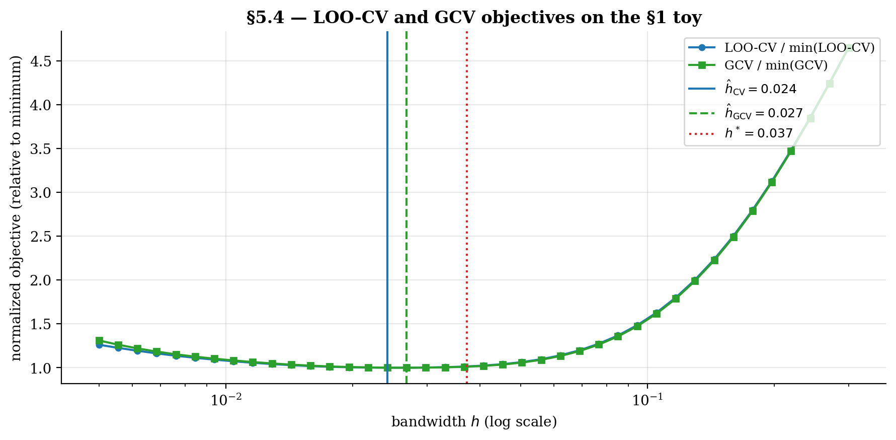
5.4 Generalized cross-validation
GCV (Craven–Wahba 1979) replaces the per-point leave-one-out adjustment with a global one:
where is the smoother matrix: with . The denominator is a degrees-of-freedom correction; the trace measures how much each observation influences its own fit.
GCV is computationally simpler than LOO-CV (no per-point adjustment, just the trace of the smoother matrix) but asymptotically equivalent to leading order. For most smoothers of practical interest, the two selectors agree to within their own variability across replicates.
The trace has a clean closed form for NW:
When the design is roughly uniform over and is small, , so — proportional to , the “effective number of parameters” the bandwidth uses up. This is the heuristic that plays the role of degrees of freedom in nonparametric regression — useful for AIC/BIC-like extensions.
5.5 Comparing selectors on the §1 toy
We compare the four selectors on a fixed sample, then assess stability across replicate samples. Two questions:
- On a single sample, how do the selectors compare to the analytical AMISE optimum?
- Across replicates, how variable is each selector’s bandwidth choice?
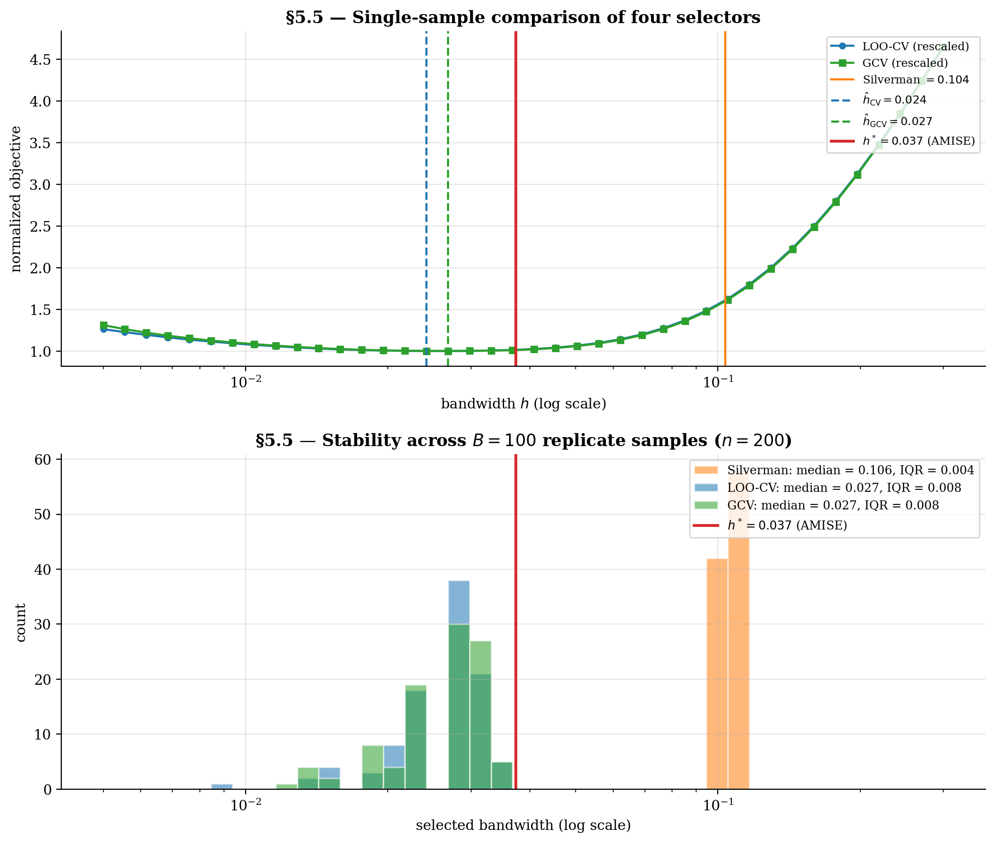
Silverman is essentially deterministic — it depends only on , which has small variance for . LOO-CV and GCV inherit non-trivial variance from the slow convergence rate. The AMISE-optimal is fixed (a property of the DGP, not the sample).
The viz below runs the head-to-head comparison and the stability experiment. Toggle individual selectors to isolate their behavior; scrub and to see how stability scales.
Top: a single sample's LOO-CV and GCV objective curves nearly coincide; their minimizers (vertical markers) sit close to the analytical h^* (dashed red). Silverman's rule lands well to the right — oversmoothed because it targets density estimation, not regression. Bottom: stability across B replicates. Silverman is essentially deterministic; LOO-CV and GCV inherit the slow n^(-3/10) variance and spread out, but their median tracks h^*.
6. Multivariate regression and the curse of dimensionality
The bias-variance machinery from §3–§4 extends naturally from to , but with one critical change: the kernel-neighborhood volume scales as , so the effective number of points within one bandwidth shrinks exponentially in dimension. The AMISE rate becomes — slower than the parametric at any , and noticeably slower than the rate once gets above 2 or 3. This is the curse of dimensionality.
We work through the multivariate extension in §6.1–6.2, derive the AMSE rate in §6.3 with empirical verification at , and state Stone’s minimax-optimality theorem in §6.4 — the result that says the curse is fundamental, not a defect of NW.
6.1 Product kernels in
For multivariate , the simplest multivariate kernel is a product of univariate kernels:
where is a univariate kernel from Definition 1 and we use a single isotropic bandwidth for all coordinates.
The Nadaraya–Watson estimator generalizes:
The kernel moment conditions extend coordinate-wise: , , and (diagonal — no cross-correlations from a product kernel). The kernel-second-moment integral becomes
The exponent in is the first hint of the curse: the variance constant grows exponentially in dimension. We see the load-bearing factor in the variance formula in §6.3. A sanity check: in , the multivariate NW reduces exactly to the univariate NW from §2, with maximum gap across a 400-point grid.
6.2 Bandwidth matrices and anisotropy
Real data often has different scales or smoothness across coordinates. Two extensions of the scalar bandwidth handle this.
Anisotropic product kernel. Per-coordinate bandwidths :
The bandwidths can be tuned individually — typically by per-coordinate Silverman or coordinate-wise cross-validation.
Full bandwidth matrix. A positive-definite matrix rotates and scales the kernel ellipsoid:
This handles correlated covariates: when and are strongly correlated, an axis-aligned product kernel under-uses the joint information; rotating to the principal-component basis recovers it.
In practice these refinements adjust the constant in front of the AMISE rate but rarely change the rate itself. The asymptotic curse-of-dimensionality story in §6.3 is unchanged whether we use a scalar bandwidth, an anisotropic product kernel, or a full bandwidth matrix. We focus on the isotropic case in §6.3–6.4 because it cleanly exposes the rate.
A pragmatic compromise that captures most of the gain available from anisotropy without the full machinery: rescale each coordinate to unit variance via , then use an isotropic bandwidth on the rescaled data. This is the multivariate analog of Silverman’s rule.
6.3 The AMSE rate
The bias-variance decomposition extends from §3–§4 with the following changes.
Bias. Replace the single-coordinate with the trace of the Hessian , and the design-density correction with :
Same rate as in .
Variance. The kernel “neighborhood” has volume , so the effective number of points within one bandwidth is :
The in the denominator is the load-bearing change. As increases, the kernel needs to be much wider to capture enough points, but wider kernels mean higher bias.
AMISE. Combining squared bias and variance:
Differentiating: , giving
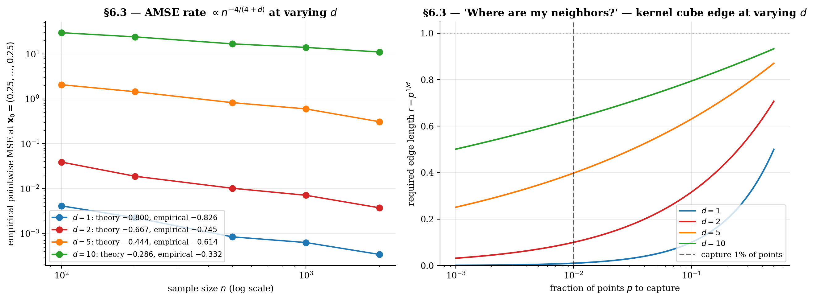
The curse of dimensionality is the rate slowing as grows. To halve the AMISE in dimensions, multiply by : at , at , at , at .
Geometric intuition. In , capturing fraction of uniform random points within an axis-aligned hypercube of edge requires . To capture 1% of points: in , in , in , in . The kernel “neighborhood” stops being local — at it consumes most of the support to find any neighbors at all.
The viz below verifies the rate empirically across at the test point on the multivariate sin-sum toy. The left panel shows the empirical AMSE-vs- slopes; the right panel shows the kernel-cube edge that quantifies “where are my neighbors.”
At d = 1 the AMSE line drops with slope close to −0.8 (one decade of n buys ~6× lower error). Crank d to 10: the slope flattens to −0.29 — the same factor of n improvement only buys ~2×. The right panel is the geometric face of this: a "local" kernel neighborhood at d = 10 spans >60% of each axis to capture even 1% of uniform points.
6.4 Stone’s minimax-optimality theorem
Stone (1980, 1982) proved a strong negative result.
Theorem 4 (Stone's minimax-optimality (1980, 1982)).
For the class of -times-continuously-differentiable functions on with bounded derivatives, no estimator can achieve a uniform convergence rate faster than in the minimax sense.
For — the standard regularity assumed throughout §3–§4 — this rate is exactly , the rate kernel regression achieves with a second-order kernel.
So NW is rate-optimal in the minimax sense for functions. The curse of dimensionality isn’t a defect of the estimator — it’s a fundamental information-theoretic property of nonparametric regression. Without assuming more structure on , no method (kernel, spline, neural network, anything) can do better in the worst case.
The rate-versus-smoothness ladder:
- -times-differentiable, second-order kernel: — what NW achieves.
- -times-differentiable, -th-order kernel (with for ): . Faster for smoother , but higher-order kernels take negative values and lose interpretability.
- Lipschitz only (): — slower than NW.
- Compositionally structured (additive models, deep networks under approximation theory, etc.): potentially much faster, depending on the structural assumption.
The takeaway is concrete. Kernel regression is rate-optimal at or so, useful but slow at , and impractical at without additional structure on . The standard structural alternatives — additivity, sparsity, single-index models, deep compositional structure — are themselves the subject of T2 Supervised Learning’s later topics. We connect kernel regression to its broader family of methods in §9.
7. Kernel choice: what matters and what doesn’t
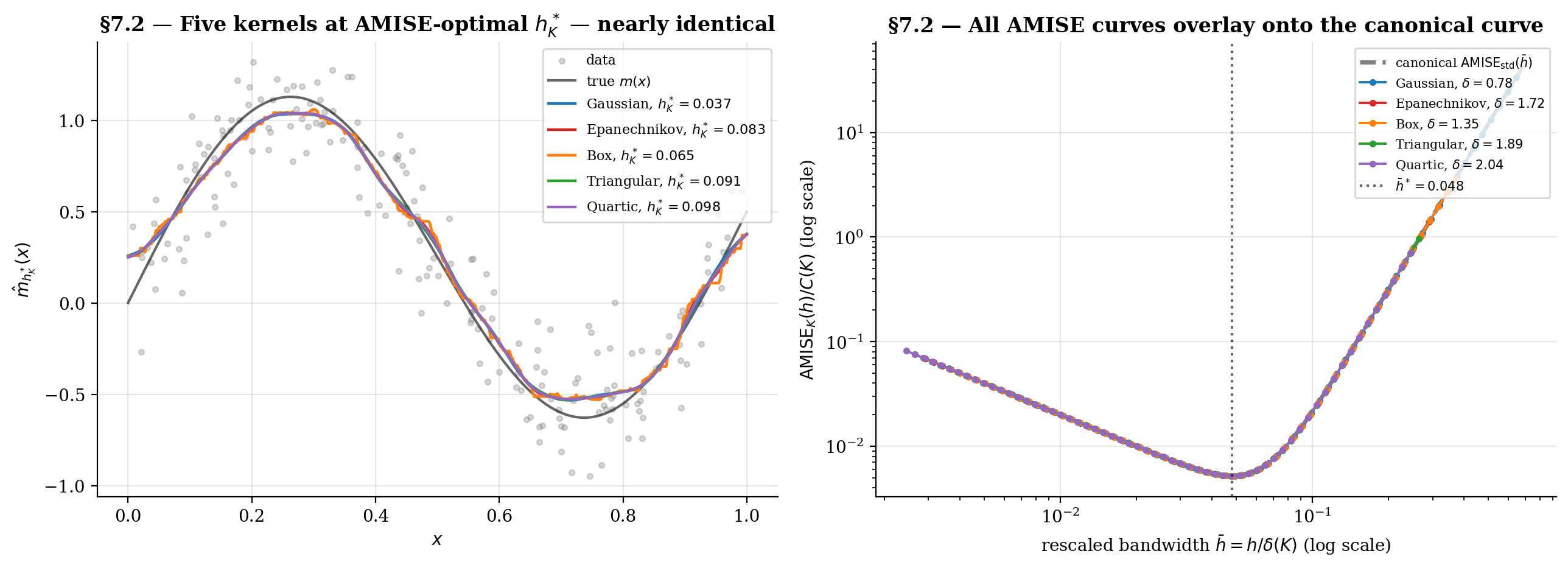
This section finishes the story §2.1 started — comparing the five standard kernels and quantifying how much kernel choice actually matters. The headline result is the canonical-kernel theorem (Marron–Nolan 1988): when each kernel uses its own AMISE-optimal bandwidth, the resulting NW smoothers are nearly indistinguishable. Kernel shape is essentially a calibration choice for the bandwidth, not an estimator-design choice. The exception is the box kernel, which inherits §1.3’s jaggedness even at its optimal bandwidth.
We tabulate the kernel-quality constants and in §7.1, derive and verify the canonical-kernel theorem in §7.2, and discuss the practical exceptions in §7.3.
7.1 The standard zoo: Gaussian, Epanechnikov, box, triangular, quartic
Recall the five kernels introduced in §2.1: Gaussian , Epanechnikov , box , triangular , and quartic .
The viz below tabulates four kernel-quality constants:
- — second moment, controls the bias (§3).
- — kernel-second-moment integral, controls the variance (§4).
- — canonical bandwidth (defined in §7.2).
- — kernel-efficiency constant.
The first two come from §2.1’s numerical integration; the last two are simple combinations. Toggle individual kernels to isolate their behavior; switch between canonical mode (each kernel uses its own ) and shared- mode (all kernels share one user-chosen ) to see the canonical-kernel theorem in action.
| Kernel | μ₂(K) | R(K) | δ(K) | C(K) | h*_K |
|---|---|---|---|---|---|
| Gaussian | 1.0000 | 0.2821 | 0.7764 | 0.3633 | 0.0373 |
| Epanechnikov | 0.2000 | 0.6000 | 1.7188 | 0.3491* | 0.0826 |
| Box | 0.3333 | 0.5000 | 1.3510 | 0.3701 | 0.0649 |
| Triangular | 0.1667 | 0.6667 | 1.8882 | 0.3531 | 0.0908 |
| Quartic | 0.1429 | 0.7143 | 2.0362 | 0.3508 | 0.0979 |
*Epanechnikov minimizes C(K) — the Hodges-Lehmann optimality result.
Toggle "canonical h^*_K" off and pick a common h to see the smoothers diverge — box produces a piecewise-constant zigzag, Gaussian smooths most heavily, Epanechnikov sits in between. Toggle it on, and at each kernel's own AMISE-optimal h^*_K, the curves nearly overlap. That's the canonical-kernel theorem (Marron-Nolan 1988): kernel choice is mostly a calibration on h.
7.2 Asymptotic equivalence and the canonical kernel
The AMISE-optimal bandwidth from §4.4 is
For two kernels on the same problem (, , shared), the ratio of optimal bandwidths is
is the canonical bandwidth of — a kernel-specific, problem-independent rescaling factor. Define the rescaled bandwidth .
Theorem 5 (Canonical-kernel theorem (Marron–Nolan 1988)).
With and ,
Up to the multiplicative constant and the bandwidth rescaling , all NW smoothers with kernels satisfying the standard moment conditions behave identically.
Proof.
Substitute into the AMISE formula from §4.3:
The bias-squared term becomes
Using , we get . Wait — more directly: . So the bias-squared term equals .
Similarly, the variance term:
using .
Combining: , as claimed.
∎Two consequences. The optimal rescaled bandwidth is kernel-independent — every kernel shares the same optimum in canonical units. The AMISE value at the optimum scales by — different kernels achieve different AMISE values, but the shape of the AMISE-vs- curve is identical.
Epanechnikov optimality (Hodges–Lehmann 1956 / Epanechnikov 1969): among kernels satisfying the standard moment conditions, the Epanechnikov kernel minimizes . Other kernels lose 1–7% efficiency relative to Epanechnikov, as the §7.1 table shows.
7.3 When kernel choice actually moves the needle
Three settings where kernel choice does matter despite the canonical-kernel theorem.
At suboptimal bandwidth. The theorem says kernels are equivalent at their respective optima. If you fix one bandwidth across kernels (say for all), the smoothers can differ noticeably because different kernels have different effective neighborhoods at the same . The §1.3 box-vs-Gaussian comparison at matched bandwidth was an instance of this — both achieve smooth fits at their respective optima, but at the same the box looks much rougher because its effective rescaled bandwidth is different. In practice this means: don’t compare kernels at the same — compare each at its own AMISE-optimal .
Box-kernel jaggedness. Even at its AMISE-optimal bandwidth, the box kernel produces a piecewise-constant smoother because the indicator-function weighting is discontinuous in the target point. This is a finite- artifact, not asymptotic — the box kernel converges to the true at the same rate as the others, but the per-sample smoother always has visible jumps. Avoid the box for any application where smoothness of matters, including visualization and derivative estimation.
Higher-order kernels. Beyond the standard second-order family, higher-order kernels — those with for and — can achieve faster convergence rates () when is sufficiently smooth (-times differentiable). A fourth-order example: . These take negative values, can produce outside the range of the data, and lose the “weighted average” interpretability. They’re rarely used in practice except in theoretical work (Tsybakov 2009, §1.2).
Pragmatic recommendation. Use the Gaussian kernel for everyday work — smooth, no support boundary, only a 5% efficiency loss vs Epanechnikov. Use Epanechnikov when you want the AMISE optimum and can tolerate the support-boundary discontinuity. Use Quartic if you need a smoother kernel with compact support (e.g., for derivative estimation where should be continuous). Avoid the box kernel outside introductory examples. Avoid higher-order kernels unless theory specifically demands them.
8. Boundary bias and the local-linear fix
§3.4 previewed that the §3 bias derivation breaks at the boundary of the support of : the rate degrades to , an order worse. This section formalizes the breakdown via the boundary kernel moments , derives the local-linear estimator that fixes the problem by reproducing both constants and linear functions exactly, and forwards to the canonical Fan–Gijbels treatment in local-regression.
The headline result: local-linear regression has bias uniformly across the support, including at the boundary — same asymptotic rate as NW at the interior, but without the boundary degradation. It also has a cleaner interior bias formula (no design-density correction term). When deploying a kernel smoother on data, use local-linear, not Nadaraya–Watson.
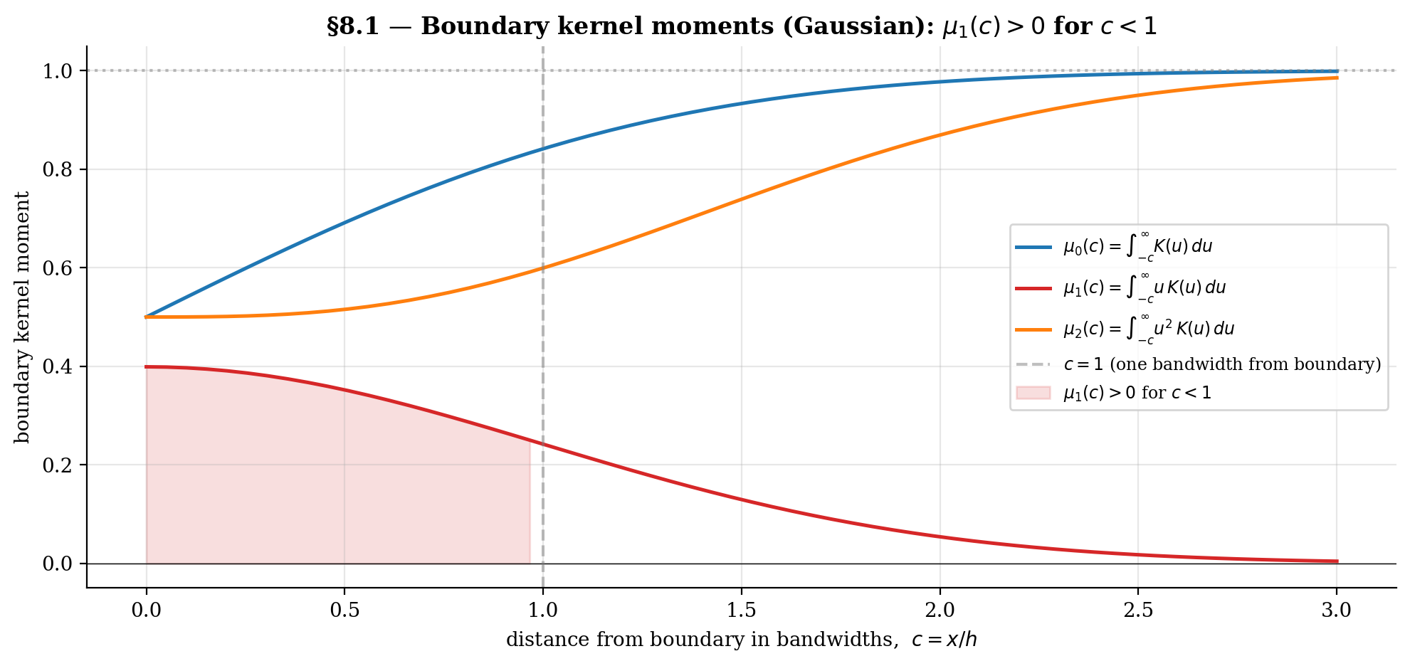
8.1 What goes wrong at the boundary of the support
Define the boundary kernel moments at distance from the boundary at :
(For compactly supported on , the upper limit becomes for ; for unbounded support like Gaussian, contributions from beyond are negligible.)
At the interior (, kernel mass entirely inside the support): , , — the standard moment conditions from Definition 1.
At a boundary point (, kernel partially outside the support): , , . The zero-first-moment condition fails — this is what kills the §3 derivation.
The Taylor expansion of from §3.2 picks up a non-vanishing linear-in- term at the boundary:
and similarly for . After the ratio expansion, the leading-order bias is
instead of the interior . For the §1 toy at (i.e., ) with the Gaussian kernel: . With , the leading-order boundary bias at is — exactly the order-of-magnitude §3.4 found empirically.
8.2 Local-linear regression as the leading-order correction
The fix: instead of fitting a constant in the kernel-weighted neighborhood (degree-zero local polynomial = NW), fit a line (degree-one local polynomial = local-linear regression).
At target , solve
and define . The slope estimate approximates but isn’t used directly — we discard it and keep only the intercept.
Define the kernel-weighted moments for and for . The LL estimate is
Lemma 2 (Local-linear weights reproduce constants and linear functions).
Equivalently, with adjusted weights satisfying
The first identity says LL reproduces constants (same as NW). The second says LL reproduces linear functions — the new property. Together these are the discrete analogs of and . The LL weights restore the zero-first-moment condition automatically, even at the boundary where the underlying kernel violates it.
Theorem 6 (Bias of local-linear regression (Fan 1992, Ruppert–Wand 1994)).
Under the conditions of Theorem 1, at the interior
This is simpler than NW’s interior bias — the design-density correction from Theorem 1 is gone. At the boundary the bias is still with a different boundary-corrected coefficient. So the bias is uniformly across the support — the boundary problem is fixed.
Variance of LL. Same order as NW: , with a slightly larger constant at the boundary.
The vectorized implementation is a small extension of NW — accumulate the kernel-weighted moments in a single sweep, then a closed-form solve per evaluation point:
def local_linear(X, Y, x_eval, h, K=K_gaussian):
"""Local-linear regression, vectorized over x_eval."""
diff = X[None, :] - x_eval[:, None] # shape (|x_eval|, n)
w = K(diff / h) / h
s0 = w.sum(axis=1)
s1 = (w * diff).sum(axis=1)
s2 = (w * diff**2).sum(axis=1)
t0 = (w * Y[None, :]).sum(axis=1)
t1 = (w * diff * Y[None, :]).sum(axis=1)
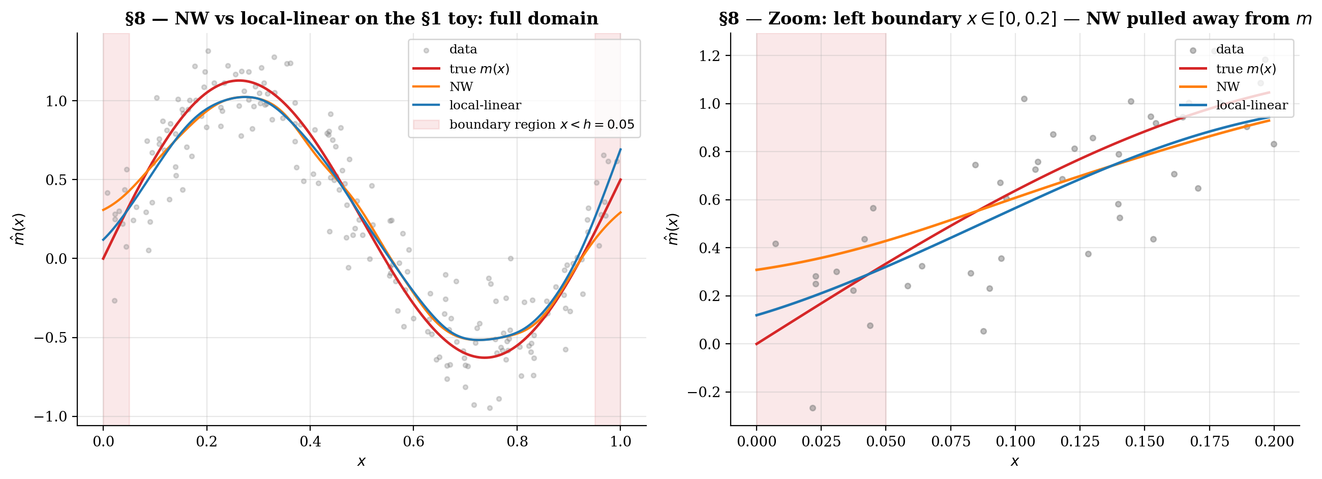
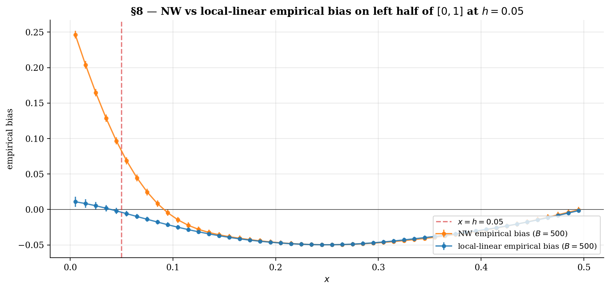
return (s2 * t0 - s1 * t1) / (s0 * s2 - s1**2)The viz below shows NW vs LL fits with the boundary regions shaded; the bottom panel plots empirical bias as a function of from replicates. NW pulls dramatically away from inside the boundary regions; LL stays close.
At interior x both estimators have O(h²) bias and visibly track each other. Inside the shaded boundary regions the NW curve breaks down to O(h) — the kernel mass falls off the support and the estimator pulls toward the side where data exists. Local-linear fixes this by reproducing both constants AND linear functions exactly under any kernel weights; boundary bias stays O(h²) uniformly.
8.3 Forward pointer: local-regression (Fan–Gijbels)
Local-linear is the simplest member of a family — degree- local polynomial regression. The general estimator solves
with . The Fan–Gijbels (1996) book is the canonical treatment. Three key results:
Even degrees offer no boundary improvement over the next-lower odd degree. So degree-2 (local-quadratic) at the interior matches LL at the boundary, while degree-3 (local-cubic) at the interior is what’s needed to match local-quadratic at the boundary. The standard practical choice is degree (local-linear) — the simplest estimator that fixes the boundary problem without adding complexity.
Higher-degree local polynomials achieve faster rates ( for odd in ) under stronger smoothness, paralleling the higher-order kernel story from §7.3. Rarely useful in practice.
The equivalent-kernel formulation. Every local-polynomial estimator can be rewritten as a kernel smoother where depends on — it’s location-adaptive. NW’s equivalent kernel is just ; LL’s equivalent kernel is automatically boundary-corrected (and at the interior reduces to exactly).
Local Polynomial Regression derives the boundary-corrected bias formula explicitly, develops the equivalent-kernel formulation that recasts every degree- estimator as a kernel smoother with a degree-aware reweighting, proves the Ruppert–Wand (1994) bias rate at odd uniformly across the support, and lands on the recommendation. It extends to multivariate covariates (with the curse-of-dimensionality penalty), gives derivative estimates as a single-fit byproduct, proves Silverman’s (1984) asymptotic equivalence between cubic smoothing splines and local-cubic regression, and bridges to GAMs via backfitting on the partial residuals.
For the present topic, the takeaway is concrete. When you actually deploy a kernel smoother on data, use local-linear, not Nadaraya–Watson. It costs nothing extra computationally (one linear solve per evaluation point), it has the same asymptotic rate at the interior, it eliminates the design-density correction term in the bias, and it fixes the boundary-bias problem entirely. Nadaraya–Watson is the right pedagogical entry point — it’s the simplest kernel smoother and the one that makes the bias-variance machinery cleanest to derive — but local-linear is the production estimator.
9. Connections and applications
The Nadaraya–Watson estimator sits in a rich ecosystem of related methods. This section maps four explicit connections — kernel ridge regression as the RKHS counterpart, Gaussian-process regression as the Bayesian counterpart, semi-parametric inference as the most common ML application, and conformal prediction as the natural way to construct distribution-free prediction intervals — plus a forward pointer to T2’s density-ratio-estimation.
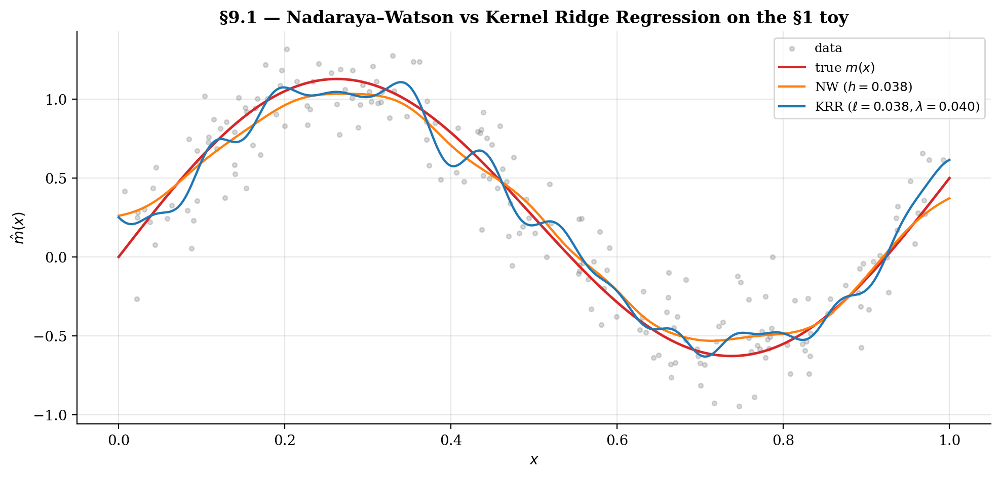
9.1 Kernel ridge regression as the RKHS counterpart
Kernel ridge regression (KRR) fits a function in a Reproducing Kernel Hilbert Space (RKHS) with a norm penalty:
The Representer Theorem reduces this infinite-dimensional optimization to a finite linear system: the minimizer takes the form , where the coefficients solve
with the Gram matrix and a regularization parameter. So KRR is a closed-form linear-algebra solution, parallel in spirit to NW but quite different in mechanics.
KRR vs NW. Both methods use kernels but apply them differently. NW computes a kernel-weighted average of the ‘s; KRR solves a regularized least-squares problem in the RKHS. NW’s smoothing parameter is the bandwidth ; KRR’s is the regularization (and the kernel may carry its own length-scale parameter ). NW weights sum to at every target — interpretable as a weighted average; KRR weights don’t have this property in general. As , KRR interpolates the data (overfits); as , KRR shrinks to a constant (oversmooths). NW’s bandwidth plays the analogous role: over-fits, over-smooths.
Asymptotic equivalence. For squared-exponential kernel with length scale and ridge , KRR has bias and variance in — same rates as NW with . KRR can also be derived as the MAP estimate under a Gaussian-process prior with kernel and noise variance — the bridge to §9.2.
9.2 Gaussian-process regression as the Bayesian counterpart
Place a Gaussian-process prior on the regression function and observe with . The closed-form posterior at a test point is Gaussian with mean and variance
The posterior mean is identical to KRR with . The GP is the Bayesian view of the same point estimate; KRR is the frequentist regularized-RKHS view. Same prediction; the GP additionally provides a posterior variance for uncertainty quantification.
NW vs GP. NW is like a GP posterior mean where the implicit prior is a “kernel-density-like” object rather than a proper GP. NW lacks the formal Bayesian interpretation but produces qualitatively similar fits at well-chosen bandwidths. The §4.4 asymptotic CI for NW is the analog of GP’s posterior variance, derived from frequentist asymptotic-normality theory.
For the full Bayesian treatment — GP as a prior over functions, posterior inference, hyperparameter learning via marginal likelihood, kernel design (Matérn, periodic, ARD), scaling tricks (sparse GPs, inducing points, SVGP) — see Gaussian Processes in T5 Bayesian ML. GPs sit in T5 rather than T2 because they’re properly Bayesian estimators, but they share the kernel-methods substrate with this topic and with KRR.
9.3 Smoothing in semi-parametric inference
Semi-parametric models combine parametric and nonparametric components. Three common forms:
- Partial linear model , with unknown and estimated nonparametrically.
- Single-index model .
- Varying-coefficient model , with a smooth function of .
In all three, kernel smoothing handles the nonparametric component and a parametric estimator handles the rest.
The key trade-off. Kernel regression converges at in — slower than the parametric . To recover for the parametric component in a semi-parametric model, the nonparametric component must be undersmoothed — bandwidth chosen smaller than AMISE-optimal so that bias doesn’t contaminate the parametric estimator.
This is the Robinson (1988) double-residual approach for partial linear models: regress on nonparametrically, regress on nonparametrically, then OLS the residuals against each other. The undersmoothing condition ensures the kernel bias is asymptotically negligible against the OLS noise.
The modern double-machine-learning literature (Chernozhukov et al. 2018) generalizes this to high-dimensional plug-in nuisance estimation. The kernel regression at the heart of the double-residual machinery can be replaced by lasso, random forests, neural networks — but the orthogonality-and-undersmoothing logic carries over directly.
The general principle: AMISE-optimal bandwidth is right for prediction; it’s wrong for inference about a parametric component. When you’re using NW as a tool inside a larger inferential procedure, the optimal bandwidth depends on what the inferential target is — not always what the kernel regression itself is solving.
9.4 Conformal-prediction interval construction
Conformal prediction (Vovk, Gammerman & Shafer 2005) gives finite-sample, distribution-free prediction intervals for any base estimator. The key idea: calibrate prediction-interval widths from out-of-sample residuals on held-out data.
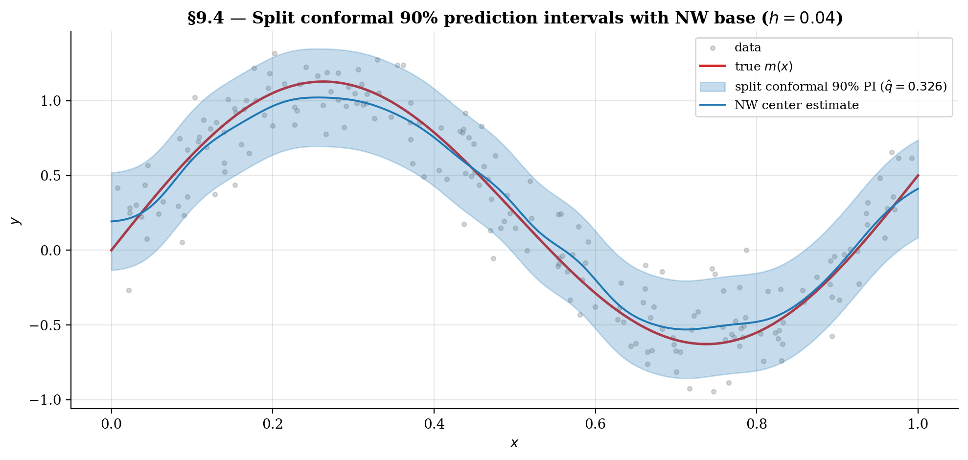
Algorithm 1 (Split-conformal NW prediction interval).
Given training data , miscoverage level , bandwidth , and a new test point :
- Permute the data and split into proper training set and calibration set , typically 50/50.
- Fit the NW estimator on .
- Compute calibration residuals for .
- Compute — the -th smallest residual (with the finite-sample correction).
- Return the prediction interval .
The finite-sample-corrected quantile in step 4 is what makes the marginal-coverage guarantee exact:
for any joint distribution over and any base estimator . No assumption that NW is correctly specified, no asymptotic regularity conditions — just exchangeability of the calibration sample and the new test point.
Connection to kernel regression. Kernel regression is a natural base estimator for conformal prediction: the NW smoother is differentiable in the data and tends to produce calibration residuals that vary smoothly in , which is what the locally-adaptive variants of conformal prediction (Lei et al. 2018) exploit. The §4.4 asymptotic-normality CI is a parallel construction with stronger assumptions — it uses the NW asymptotic distribution to construct the interval — and produces tighter intervals at the cost of distribution-free guarantees.
For full coverage of the conformal machinery — split conformal, jackknife+, CV+, locally-adaptive conformal, conformal classification — see Conformal Prediction in T4 Nonparametric & Distribution-Free.
9.5 Forward pointer: density-ratio-estimation (KLIEP / LSIF / uLSIF)
The next T2 Supervised Learning topic after local-regression is density-ratio-estimation — estimating from samples of and without estimating either density separately. Three classical kernel-based approaches:
- KLIEP (Sugiyama et al. 2008) — minimizes over a kernel basis. Iterative.
- LSIF (Kanamori, Hido & Sugiyama 2009) — least-squares importance fitting in a kernel basis. Closed-form.
- uLSIF (Kanamori, Hido & Sugiyama 2009) — unconstrained LSIF, dropping the positivity constraint for numerical stability. Closed-form, the practical favorite.
All three use the same kernel machinery as kernel regression: same kernel families (Gaussian, Epanechnikov), same bandwidth-selection considerations (LOO-CV, GCV port over directly), same curse of dimensionality. The mathematical structure is parallel — instead of estimating , we estimate , but both are conditional functionals of underlying density estimates and both are well-served by the same kernel-weighted-least-squares framework.
Applications of density-ratio estimation: covariate-shift correction in supervised learning (where train and test distributions differ); change-point detection in time series; anomaly detection (low ratio signals out-of-distribution); off-policy evaluation in reinforcement learning (importance ratio of behavior to target policy); importance-weighted classification; two-sample tests (the ratio acts as a test statistic).
Connections and Further Reading
Within formalML, this topic feeds into:
-
Local Polynomial Regression. The Fan–Gijbels boundary-bias fix from §8, generalizing local-linear to higher-degree polynomials with full coverage of the equivalent-kernel formulation , the Ruppert–Wand (1994) bias ladder, the odd-vs-even degree story, multivariate extension, derivative estimation, and the connection to GAMs via backfitting. The kernel-methods shared module from this topic is the substrate.
-
Density-Ratio Estimation (coming soon). KLIEP / LSIF / uLSIF importance-ratio estimators that use the kernel machinery from §2 and the bandwidth-selection methods from §5 for a parallel functional ( instead of ) — see §9.5.
-
Gaussian Processes (T5). The Bayesian counterpart of kernel ridge regression; same closed-form posterior mean as KRR with , plus a closed-form posterior covariance for uncertainty quantification — see §9.2.
-
Conformal Prediction (T4). Finite-sample distribution-free prediction intervals using NW (or any base estimator) at the calibration step — see §9.4 and Algorithm 1.
Cross-site prerequisites:
-
formalStatistics: Kernel Density Estimation — the density-estimation sibling. Same kernel moment conditions (∫K = 1, ∫uK = 0, μ₂(K)) and the same h² bias / 1/(nh) variance machinery, applied to instead of . The Silverman bandwidth heuristic in §5.1 is the KDE rule applied directly. The §3 bias derivation runs in parallel to KDE’s: same Taylor expansion, same change of variables.
-
formalStatistics: Linear Regression — the parametric counterpart. The §2.3 NW-as-WLS reframing draws directly on weighted-least-squares theory; the §8.2 local-linear extension is locally-weighted OLS with two parameters.
-
formalCalculus: Multiple Integrals — the multivariate-integration toolkit. The change-of-variables substitution used throughout §3.2 and the d-dimensional volume scaling in §6.3 are standard multivariate-integration moves; the §6.1 product-kernel identity uses Fubini.
-
formalCalculus: Mean Value Theorem and Taylor Expansion — the Taylor-expansion machinery. The §3.2 second-order expansion of and around , with explicit remainder, is the load-bearing technical move of the entire bias derivation. The §6.3 multivariate version uses the same expansion with the Hessian replacing the second derivative.
Internal prerequisites:
- Concentration Inequalities. Direct prerequisite for the convergence-rate machinery. The §3 bias and §4 variance derivations are stated to leading order, but the rigorous version (uniform consistency, asymptotic normality) requires concentration-inequality bounds for the kernel-weighted partial sums. Concentration inequalities provide the Hoeffding/Bernstein machinery that justifies the leading-order approximations used throughout §3–§6.
Connections
- Direct prerequisite for the convergence-rate machinery. The §3 bias and §4 variance derivations are stated to leading order, but the rigorous version (uniform consistency) requires concentration-inequality bounds for the kernel-weighted partial sums. concentration-inequalities provides the Hoeffding/Bernstein machinery that justifies the leading-order approximations used throughout §3-§6. concentration-inequalities
- GP regression's posterior mean is identical to KRR with λ = σ². §9.1-9.2 develop the connection: NW is the kernel-weighted-average sibling of GP/KRR; both use the same kernel families (RBF, Matérn, etc.) but differ in how the weights are computed. §9.2 forwards readers to the gaussian-processes topic for the full Bayesian treatment. gaussian-processes
- §9.4 implements split conformal prediction with NW as the base estimator on the §1 toy and verifies the marginal-coverage guarantee empirically. Conformal prediction's distribution-free finite-sample guarantee complements NW's asymptotic-normality CI from §4.4. The kernel-regression topic provides the natural base estimator for conformal prediction's smoothing step. conformal-prediction
References & Further Reading
- paper The efficiency of some nonparametric competitors of the t-test — Hodges, J. L., Jr. & Lehmann, E. L. (1956)
- paper On estimating regression — Nadaraya, E. A. (1964)
- paper Smooth regression analysis — Watson, G. S. (1964)
- paper Non-parametric estimation of a multivariate probability density — Epanechnikov, V. A. (1969)
- paper Smoothing noisy data with spline functions: estimating the correct degree of smoothing by the method of generalized cross-validation — Craven, P. & Wahba, G. (1979)
- paper Optimal rates of convergence for nonparametric estimators — Stone, C. J. (1980)
- paper Optimal global rates of convergence for nonparametric regression — Stone, C. J. (1982)
- paper Optimal bandwidth selection in nonparametric regression function estimation — Härdle, W. & Marron, J. S. (1985)
- book Density Estimation for Statistics and Data Analysis — Silverman, B. W. (1986)
- paper Canonical kernels for density estimation — Marron, J. S. & Nolan, D. (1988)
- paper Root-N-consistent semiparametric regression — Robinson, P. M. (1988)
- book Applied Nonparametric Regression — Härdle, W. (1990)
- paper Local minima in cross-validation functions — Hall, P. & Marron, J. S. (1991)
- paper Design-adaptive nonparametric regression — Fan, J. (1992)
- paper Multivariate locally weighted least squares regression — Ruppert, D. & Wand, M. P. (1994)
- paper An effective bandwidth selector for local least squares regression — Ruppert, D., Sheather, S. J. & Wand, M. P. (1995)
- book Kernel Smoothing — Wand, M. P. & Jones, M. C. (1995)
- book Local Polynomial Modelling and Its Applications — Fan, J. & Gijbels, I. (1996)
- paper Using the Nyström method to speed up kernel machines — Williams, C. K. I. & Seeger, M. (2001)
- book Algorithmic Learning in a Random World — Vovk, V., Gammerman, A. & Shafer, G. (2005)
- paper Random features for large-scale kernel machines — Rahimi, A. & Recht, B. (2007)
- paper Direct importance estimation for covariate shift adaptation — Sugiyama, M., Suzuki, T., Nakajima, S., Kashima, H., von Bünau, P. & Kawanabe, M. (2008)
- paper A least-squares approach to direct importance estimation — Kanamori, T., Hido, S. & Sugiyama, M. (2009)
- book Introduction to Nonparametric Estimation — Tsybakov, A. B. (2009)
- paper Distribution-free predictive inference for regression — Lei, J., G'Sell, M., Rinaldo, A., Tibshirani, R. J. & Wasserman, L. (2018)
- paper Double/debiased machine learning for treatment and structural parameters — Chernozhukov, V., Chetverikov, D., Demirer, M., Duflo, E., Hansen, C., Newey, W. & Robins, J. (2018)