Sequential Monte Carlo

§1. Overview and Motivation

We’re going to track a cloud of particles through a sequence of probability distributions. At each step we update each particle’s weight, occasionally throw out the low-weight ones and replicate the high-weight ones, and then jitter the survivors with a Markov move that respects the current target. Do that $T$ times against a well-chosen schedule of intermediate targets and you have sequential Monte Carlo — an algorithm that handles filtering on state-space models, sampling from intractable static posteriors, and unbiased estimation of marginal likelihoods, all with the same three moves and the same dozen lines of inner-loop code.

The geometric picture is worth holding onto. Imagine a fixed-size swarm of points $\{\theta^{(i)}\}_{i=1}^N$ in parameter space, each carrying a non-negative weight $w^{(i)}$. The weighted swarm represents the current distribution: high-weight clusters mark high-probability regions; the expectation of any test function $f$ under the current target is approximately $\sum_i w^{(i)} f(\theta^{(i)})$. As we slide the target distribution — making it sharper, or conditioning on more data, or bridging from a tractable prior to an intractable posterior — the swarm has to track it. SMC is the recipe for moving the swarm.

The topic delivers three structurally distinct uses of that one recipe:

• Particle filtering on hidden Markov / state-space models, where the sequence of targets is the filtering posterior $p(x_t \mid y_{1:t})$ and the algorithm generalizes the Kalman filter to non-linear and non-Gaussian dynamics. We demo on a stochastic-volatility model where Kalman doesn’t apply.
• SMC samplers in the Del Moral, Doucet, and Jasra (2006) sense, where we bridge a tractable prior to an intractable posterior along a synthetic annealing path $\pi_t \propto \pi_0^{1-\beta_t}\,\pi_T^{\beta_t}$. The headline payoff: an unbiased estimator of the log marginal likelihood falls out as a side product, no extra work. We demo on a Gaussian-mixture model evidence calculation and a banana-shaped two-dimensional posterior.
• Tempered transitions with adaptive schedules, where the temperature ladder $\beta_t$ is chosen on the fly via an ESS criterion (Del Moral, Doucet, and Jasra 2012, building on Jasra, Stephens, Doucet, and Tsagaris 2011) rather than hand-tuned. We demo on a log-Gaussian Cox process where target curvature varies enough across the path that a fixed schedule wastes most of the compute.

That’s where we’re going. Let’s start with why anyone needs this — what breaks when we try to do it without the sequential structure.

1.1 Where importance sampling breaks

Standard importance sampling tells us we can estimate $\mathbb{E}_\pi[f(\theta)]$ for any target $\pi$ by drawing from a proposal $q$ and reweighting:

$$\mathbb{E}_\pi[f(\theta)] \approx \frac{\sum_{i=1}^N w^{(i)}\, f(\theta^{(i)})}{\sum_{i=1}^N w^{(i)}}, \qquad \theta^{(i)} \sim q, \quad w^{(i)} = \frac{\pi(\theta^{(i)})}{q(\theta^{(i)})}.$$

In the limit $N \to \infty$ this estimator is consistent for any $q$ whose support contains $\pi$‘s — a remarkably weak condition. So why doesn’t every Bayesian-inference paper just use it?

The answer is variance. The variance of the IS estimator is controlled by the chi-squared divergence between $q$ and $\pi$, and that divergence explodes when $q$ misses the bulk of $\pi$‘s mass. Concretely: if $\pi$ is a Gaussian centred at $5$ and $q$ is a Gaussian centred at $0$, both unit-variance, then most of $q$‘s samples land in $\pi$‘s left tail. A handful of samples that happen to drift to the right pick up enormous weights — and the normalized weights end up concentrated on one or two particles. This is weight degeneracy, and it’s the failure mode SMC is designed to fix.

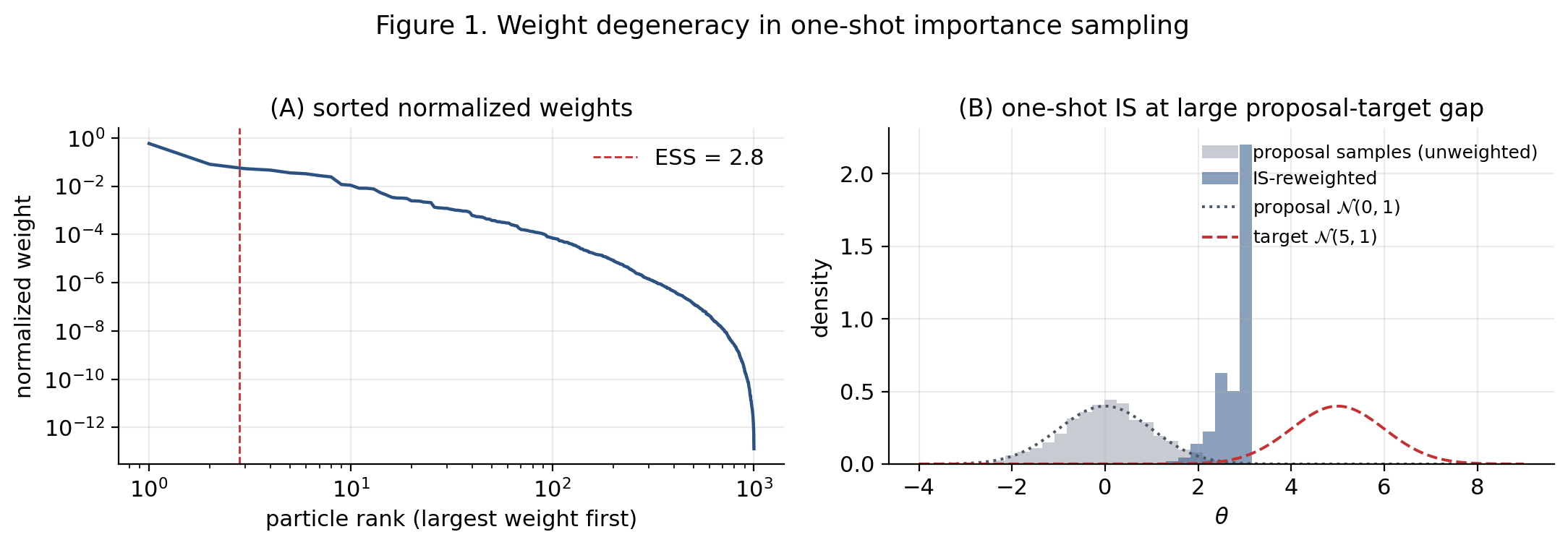
We can see it numerically with $N=1000$ (Figure 1): even a five-standard-deviation gap between proposal and target leaves an effective sample size of roughly $10$ out of $1000$, with five particles carrying more than $80\%$ of the normalized mass.

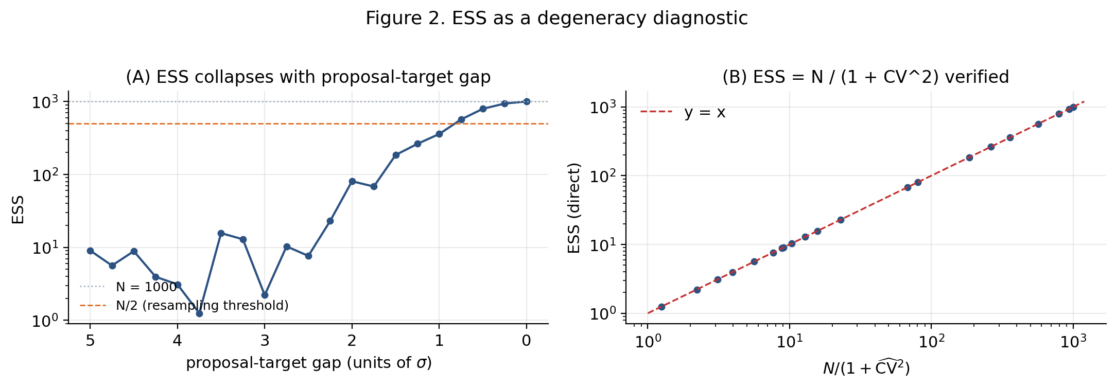
The effective sample size (ESS), defined as $\mathrm{ESS} = 1 / \sum_i (w^{(i)})^2$ on normalized weights, summarizes the damage in one number. ESS counts the number of “effective” particles — the number an iid sample from $\pi$ would need to match the IS estimator’s variance. A swarm of 1000 particles with ESS $= 3$ is contributing about as much information as 3 iid samples; the other 997 are dead weight.

The diagnosis is geometric. The proposal and target are too far apart in distribution space for a one-shot bridge. What we need is to interpolate between them.

1.2 The particle-cloud fix

The fix is structurally simple: instead of bridging $q$ to $\pi$ in one step, we build a path of intermediate distributions

$$q = \pi_0,\; \pi_1,\; \pi_2,\; \ldots,\; \pi_T = \pi$$

where adjacent targets $\pi_t$ and $\pi_{t+1}$ are close enough that a one-step importance-reweighting between them isn’t degenerate. Then we sequentially march the particle cloud from one target to the next: at step $t$, update each weight by the incremental ratio $\pi_{t+1}(\theta^{(i)})/\pi_t(\theta^{(i)})$, throw out the low-weight particles and replicate the high-weight ones (the resampling move), and apply a Markov kernel that leaves $\pi_{t+1}$ invariant to spread the survivors back out (the propagation move).

Three observations make the algorithm work:

1. Reweighting between close targets is well-conditioned. If $\pi_{t+1}$ differs from $\pi_t$ by a small amount of extra likelihood or a small temperature step, then the importance ratios $\pi_{t+1}/\pi_t$ have small variance and ESS stays $O(N)$.
2. Resampling kills the survivor bias. Without it, the cloud would still degenerate after enough steps — just more slowly than one-shot IS. Resampling preserves the weighted distribution in expectation while exchanging it for a fresh equal-weighted cloud with the same empirical measure but more degrees of freedom for the next step.
3. The Markov kernel restores diversity. Resampling duplicates particles, so we need a mutation step that moves the duplicates apart while preserving the current target. Any $\pi_{t+1}$-invariant Markov kernel works — Metropolis–Hastings, HMC, Gibbs — and the choice is essentially a hyperparameter.

The three moves — reweight, resample, propagate — are the SMC skeleton. Every variant we’ll meet is a specific way of choosing the target sequence and the propagation kernel; the skeleton itself doesn’t change.

1.3 Three uses of one skeleton

Particle filtering. Take a state-space model with latent state $x_t$, observation $y_t$, transition density $p(x_t \mid x_{t-1})$, and emission density $p(y_t \mid x_t)$. The filtering target at time $t$ is $\pi_t(x_{0:t}) = p(x_{0:t} \mid y_{1:t})$. The reweighting ratio $\pi_{t+1}/\pi_t$ is the per-observation likelihood $p(y_{t+1} \mid x_{t+1})$, and the propagation kernel is the forward transition $p(x_{t+1} \mid x_t)$. This is the bootstrap particle filter (Gordon, Salmond, and Smith 1993).

SMC samplers. Take a static target $\pi(\theta)$ and bridge from a tractable prior $\pi_0(\theta) = p(\theta)$ via the geometric annealing path $\pi_t(\theta) \propto p(\theta)\, p(y \mid \theta)^{\beta_t}$ with $0 = \beta_0 < \beta_1 < \cdots < \beta_T = 1$. The reweighting ratio is $p(y \mid \theta^{(i)})^{\beta_{t+1} - \beta_t}$, and the propagation kernel can be any $\pi_t$-invariant MCMC kernel.

Unbiased log-marginal-likelihood estimation. The SMC-samplers product $\widehat Z_T = \prod_{t=0}^{T-1} \widehat r_t$ is an unbiased estimator of the model evidence $Z_T = p(y)$, with no assumption that the sampler has converged. We prove this in §8.2.

1.4 Roadmap and what this discharges

§2 reviews just enough importance sampling to set up what SMC fixes. §3 introduces the SMC skeleton abstractly. §§4–5 catalogue the two ingredient choices — resampling schemes and propagation kernels. §6 specializes to particle filtering with the stochastic-volatility worked example. §7 specializes to SMC samplers on static targets, and §8 extracts the unbiased log-evidence estimator with the Gaussian-mixture worked example. §9 develops the two adaptive moves — ESS-thresholded resampling and adaptive temperature schedules — with the banana worked example. §10 is the convergence theory. §11 is the log-Gaussian Cox process worked example. §§12–13 are computational discipline and connections.

The topic discharges three explicit forward-pointers: formalStatistics: bayesian-computation-and-mcmc ‘s sampler catalogue and importance-sampling variance vocabulary; Probabilistic Programming §6.3’s forward-pointer to pm.sample_smc, which §§8.4 and 11.3 reproduce with a hand-rolled NumPy implementation; and Variational Bayes for Model Selection §13’s forward-pointer to SMC samplers as the unbiased alternative to ELBO-as-log-evidence, discharged here in §8.2 (Theorem 4) and §8.4 (the Gaussian-mixture benchmark).

§2. Importance Sampling at a Glance — What SMC Fixes

Importance sampling is the prerequisite, not the target. We develop SMC against it, so we need the IS vocabulary in place: the variance identity, the ESS diagnostic, and a clean statement of why the one-shot strategy fails on Bayesian targets.

2.1 The IS identity and its variance

Let $\pi$ be a probability density on $\Theta \subseteq \mathbb{R}^d$, and let $q$ be a proposal with $q(\theta) > 0$ wherever $\pi(\theta) > 0$. The importance weight at $\theta$ is $w(\theta) = \pi(\theta)/q(\theta)$. The change-of-measure identity $\mathbb{E}_\pi[f(\theta)] = \mathbb{E}_q[w(\theta) f(\theta)]$ is immediate.

The unnormalized IS estimator:

$$\hat\mu^{\,\mathrm{un}}_N = \frac{1}{N} \sum_{i=1}^N w(\theta^{(i)}) f(\theta^{(i)}), \qquad \theta^{(i)} \stackrel{\mathrm{iid}}{\sim} q,$$

is unbiased. The self-normalized IS estimator $\hat\mu^{\,\mathrm{sn}}_N = \sum_i \tilde w^{(i)} f(\theta^{(i)}) / \sum_i \tilde w^{(i)}$ (with $\tilde w^{(i)} = \gamma(\theta^{(i)})/q(\theta^{(i)})$ for unnormalized target $\gamma$) is consistent but biased at $O(1/N)$ from the delta-method Jensen gap.

The variance identity is the source of every IS pathology. The estimator is consistent for any $q$ with full support on $\pi$, but the rate is governed by $\chi^2(\pi \,\Vert\, q)$.

2.2 Effective sample size and weight degeneracy

ESS, $\widehat{\mathrm{CV}}^2$, and asymptotically the chi-squared divergence are three faces of the same diagnostic: $\mathrm{ESS}/N \to 1/(1 + \chi^2(\pi \,\Vert\, q))$ as $N \to \infty$.

2.3 Why a one-shot IS proposal fails on hard targets

The variance identity tells us we need $\chi^2(\pi \,\Vert\, q) \ll N$. In Bayesian inference the posterior $\pi_n(\theta) \propto p(\theta) \prod_j p(y_j \mid \theta)$ concentrates dramatically as $n$ grows.

Heuristic scaling. Under regularity conditions (Bernstein–von Mises), the posterior $\pi_n$ concentrates at the MLE $\hat\theta_n$ with effective volume $\sim n^{-d/2}$. The chi-squared divergence therefore scales as $\chi^2(\pi_n \,\Vert\, p) = O(n^{d/2})$ in the regular parametric setting. For irregular models the scaling is worse and can grow exponentially in $n$. We won’t formalize this further (the precise statement is the Bernstein–von Mises theorem; see van der Vaart 1998 Chapter 10 for the rigorous version), but the message is unambiguous: one-shot IS from the prior is dead on arrival.

The SMC fix is now visible by inversion. Decompose the single shot into many small shots, each with bounded chi-squared. Choose a path $\pi_0 = q,\; \pi_1,\; \ldots,\; \pi_T = \pi$ such that $\chi^2(\pi_{t+1} \,\Vert\, \pi_t) \ll N$ for each $t$. The geometric annealing path achieves this when $\beta_t$ varies slowly.

§3. The SMC Skeleton

We have the motivation (§1) and the IS toolkit (§2). Now we define the SMC algorithm abstractly — the skeleton that every specific variant in §§6–11 specializes.

3.1 A sequence of intermediate targets

Fix a final target $\pi = \pi_T$ and a tractable starting distribution $\pi_0$. Build a path of intermediate distributions $\pi_0, \pi_1, \ldots, \pi_T$ connecting the two. Three families of paths recur:

• Data-augmenting (particle filtering). $\pi_t(x_{0:t}) = p(x_{0:t} \mid y_{1:t})$. The state space grows with $t$.
• Annealing (SMC samplers). $\pi_t(\theta) \propto \pi_0(\theta)^{1-\beta_t}\,\pi_T(\theta)^{\beta_t}$ with $\beta_0 = 0 < \beta_T = 1$.
• Tempered. $\pi_t(\theta) \propto \exp(-\beta_t U(\theta))$ for a potential $U$.

Write each target as $\pi_t(\theta) = \gamma_t(\theta) / Z_t$, where $\gamma_t$ is unnormalized (tractable) and $Z_t = \int \gamma_t\, d\theta$ is the normalizing constant (typically intractable).

3.2 Reweight, resample, propagate — the three alternating moves

The SMC algorithm maintains a particle cloud $\{(\theta_t^{(i)},\, W_t^{(i)})\}_{i=1}^N$ with $\theta_t^{(i)} \in \Theta$ and $W_t^{(i)} \geq 0$. We track unnormalized cumulative weights; self-normalized weights $w_t^{(i)} = W_t^{(i)} / \sum_j W_t^{(j)}$ are derived on demand.

Initialization. Draw $\theta_0^{(i)} \stackrel{\mathrm{iid}}{\sim} \pi_0$ and set $W_0^{(i)} = 1$.

For each $t = 0, 1, \ldots, T-1$:

Move 1 (reweight). Incremental importance ratios

$$\alpha_t^{(i)} = \frac{\gamma_{t+1}(\theta_t^{(i)})}{\gamma_t(\theta_t^{(i)})}, \qquad W_{t+1}^{(i)} = W_t^{(i)} \cdot \alpha_t^{(i)}.$$

Move 2 (resample, optional and ESS-thresholded). If $\mathrm{ESS}_t < \tau N$, draw indices $A_t^{(i)} \sim \mathrm{Categorical}(w_{t+1}^{(1)}, \ldots, w_{t+1}^{(N)})$ (the specific scheme — multinomial, systematic, stratified, residual — is the topic of §4). Replace the cloud with $\{(\theta_t^{(A_t^{(i)})}, \bar W_{t+1})\}_{i=1}^N$ where $\bar W_{t+1} = \frac{1}{N}\sum_j W_{t+1}^{(j)}$.

Move 3 (propagate). Apply a Markov kernel $K_{t+1}$ that is $\pi_{t+1}$-invariant: $\int \pi_{t+1}(\theta) K_{t+1}(\theta, \theta')\, d\theta = \pi_{t+1}(\theta')$. For each particle, draw $\theta_{t+1}^{(i)} \sim K_{t+1}(\theta_t^{(A_t^{(i)})}, \cdot)$.

Terminal output. After $T$ steps, $\widehat{\mathbb{E}_{\pi_T}}[f] = \sum_i w_T^{(i)} f(\theta_T^{(i)})$ and $\widehat Z_T = \frac{1}{N}\sum_i W_T^{(i)}$.

The convention is reweight → resample → propagate, matching Del Moral, Doucet, and Jasra (2006) §3 and PyMC’s pm.sample_smc.

3.3 The weighted empirical measure

The cloud represents a probability distribution via the weighted empirical measure

$$\pi_t^N(d\theta) = \sum_{i=1}^N w_t^{(i)}\, \delta_{\theta_t^{(i)}}(d\theta).$$

Three observations. (1) $\pi_t^N$ is the algorithm’s state; tracking it is what tracking the cloud means. (2) It’s a random measure — different runs of SMC produce different particle locations and weights. (3) Special cases correspond to special algorithm states: uniform weights right after a resample, point mass when the cloud collapses to one particle.

The §10.1 consistency theorem will establish that $\pi_t^N \to \pi_t$ weakly as $N \to \infty$, with rates from the §10.3 CLT.

3.4 Notation, log-space discipline, and the cumulative-weight invariant

Symbol	Meaning
$\Theta \subseteq \mathbb{R}^d$	parameter space (or state space)
$\pi_t = \gamma_t / Z_t$	target at step $t$
$\theta_t^{(i)} \in \Theta$	particle $i$ at step $t$
$W_t^{(i)} \geq 0$, $\ell_t^{(i)} = \log W_t^{(i)}$	cumulative unnormalized weight
$w_t^{(i)} = W_t^{(i)} / \sum_j W_t^{(j)}$	self-normalized weight
$\alpha_t^{(i)} = \gamma_{t+1}/\gamma_t$ at $\theta_t^{(i)}$	incremental ratio
$K_{t+1}$	$\pi_{t+1}$-invariant Markov kernel
$\mathrm{ESS}_t = 1/\sum (w_t^{(i)})^2$	effective sample size
$\widehat Z_t = \frac{1}{N}\sum W_t^{(i)}$	running normalizing-constant estimator

Log-space discipline. Particle weights on hard targets routinely span ten or more orders of magnitude. Linear-space representation silently underflows; the implementation enforces log-space throughout:

• Store $\ell_t^{(i)} = \log W_t^{(i)}$ and update additively: $\ell_{t+1}^{(i)} = \ell_t^{(i)} + \log \gamma_{t+1}(\theta_t^{(i)}) - \log \gamma_t(\theta_t^{(i)})$.
• Normalize via logsumexp: $\log w_t^{(i)} = \ell_t^{(i)} - \mathrm{logsumexp}(\ell_t)$.
• Compute log-ESS: $\log\mathrm{ESS}_t = -\mathrm{logsumexp}(2 \log w_t)$.
• Compute log-$\widehat Z$: $\log\widehat Z_t = \mathrm{logsumexp}(\ell_t) - \log N$.

A preview of the §8.2 unbiasedness theorem. Theorem 4 in §8.2 will establish that for every $t \in \{0, 1, \ldots, T\}$,

$$\mathbb{E}\!\left[\widehat Z_t\right] = \mathbb{E}\!\left[\frac{1}{N}\sum_{i=1}^N W_t^{(i)}\right] = \frac{Z_t}{Z_0}.$$

The expectation is over all SMC randomness — initial draws from $\pi_0$, resampling indices, and Markov-kernel transitions. When $\pi_0$ is the prior (so $Z_0 = 1$), $\widehat Z_T$ is unbiased for the model evidence $Z_T = p(y)$. This is the identity that justifies all of SMC’s evidence-estimation use cases. We use it as a structural fact while developing §§4–7; the full induction proof — the topic’s most important load-bearing result — is the subject of §8.2.

Resampling preserves the invariant. Pre-resample, $\widehat Z_{t+1} = (1/N)\sum_i W_{t+1}^{(i)}$. Post-resample, each particle carries $\bar W_{t+1} = (1/N)\sum_j W_{t+1}^{(j)}$, so the new running estimator is $(1/N) \cdot N \cdot \bar W_{t+1} = \bar W_{t+1}$, identical to the pre-resample value. The resampling step is invariance-preserving by construction.

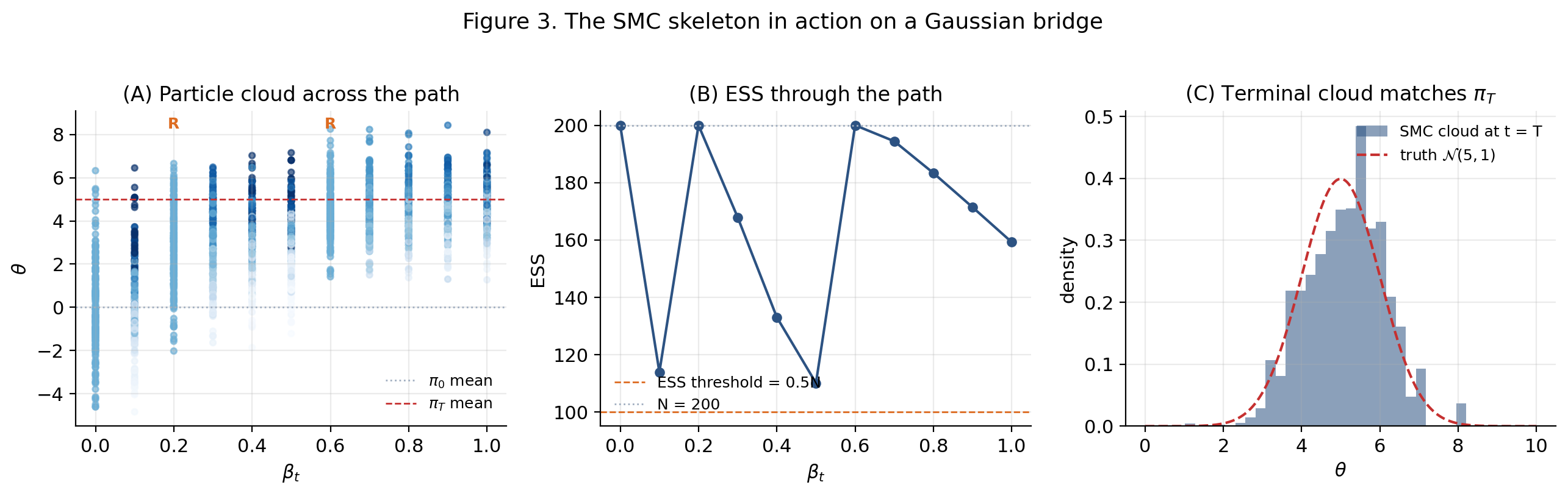
The viz below lets you change $N$, $T$, the resampling threshold $\tau$, and the RWM step size, and watch the cloud trajectory, the ESS profile, and the terminal histogram update.

N = 200T = 10τ = 0.50RWM step = 0.50

log Ẑ_T = -0.233 (truth 0)

terminal μ = 5.007 (truth 5)

terminal σ = 1.096 (truth 1)

resamples = 2 / 10

Three behaviors worth discovering: set $\tau = 0$ (never resample) and the ESS collapses by the end of the path; set $\tau = 1$ (resample every step) and the algorithm injects more variance than necessary; shrink $T = 2$ and the cloud can’t track the target. The §10.3 CLT formalizes the variance contributions of each move.

§4. Resampling Schemes

Move 2 of the skeleton — resampling — turns a degenerate weighted cloud into a fresh equal-weighted cloud. Four schemes are in common use, with a strict variance ordering:

$$\mathrm{Var}(\text{systematic}) \leq \mathrm{Var}(\text{stratified}) \leq \mathrm{Var}(\text{residual}) \leq \mathrm{Var}(\text{multinomial}).$$

All four are $O(N)$ via numpy.searchsorted. Use searchsorted, never numpy.random.choice(..., p=weights) — this is a project-wide hard rule. Systematic is the default and what PyMC’s pm.sample_smc uses.

4.1 Multinomial resampling — the naive baseline

Multinomial resampling draws $N$ ancestor indices independently:

$$A_t^{(i)} \stackrel{\mathrm{iid}}{\sim} \mathrm{Categorical}(w_t^{(1)}, \ldots, w_t^{(N)}).$$

The joint distribution of $(N_t^{(1)}, \ldots, N_t^{(N)})$ is multinomial$(N; w_t^{(1)}, \ldots, w_t^{(N)})$; the marginal of each $N_t^{(i)}$ is Binomial$(N, w_t^{(i)})$.

cumw = np.cumsum(w_norm)
u = rng.random(N)
idx = np.clip(np.searchsorted(cumw, u), 0, N - 1)

4.2 Systematic resampling (Kitagawa 1996)

Systematic resampling draws a single $u \sim U(0, 1/N)$ and uses the deterministic grid $u_k = u + k/N$. The negative association among the $u_k$ is what drives the variance reduction.

cumw = np.cumsum(w_norm)
u = (rng.random() + np.arange(N)) / N
idx = np.clip(np.searchsorted(cumw, u), 0, N - 1)

4.3 Stratified and residual resampling

Stratified resampling (Kitagawa 1996): $N$ independent uniforms, one per stratum: $u_k \sim U(k/N, (k+1)/N)$. Same code as systematic but rng.random(N) instead of rng.random().

Residual resampling (Liu and Chen 1998): deterministic integer counts $\lfloor N w^{(i)} \rfloor$, plus a residual stage via multinomial on the leftover weights.

4.4 Variance reduction — why systematic dominates multinomial

4.5 The numpy.searchsorted primitive

All four schemes reduce to one operation: given a cumulative-weight array $c$ and “uniform array” $u$, find ancestor indices via np.searchsorted(c, u). Cost: $O(N \log N)$ for $N$ queries (binary search), with excellent constants.

Why not np.random.choice(N, size=N, p=w_norm)? Three reasons: (1) performance — np.random.choice is 3–10× slower with allocator pressure on every call; (2) it only does multinomial — the worst scheme by Theorem 2; (3) GC pressure — fresh allocation each call vs reusable cumw buffer.

Project rule: always searchsorted, never np.random.choice with p=weights.

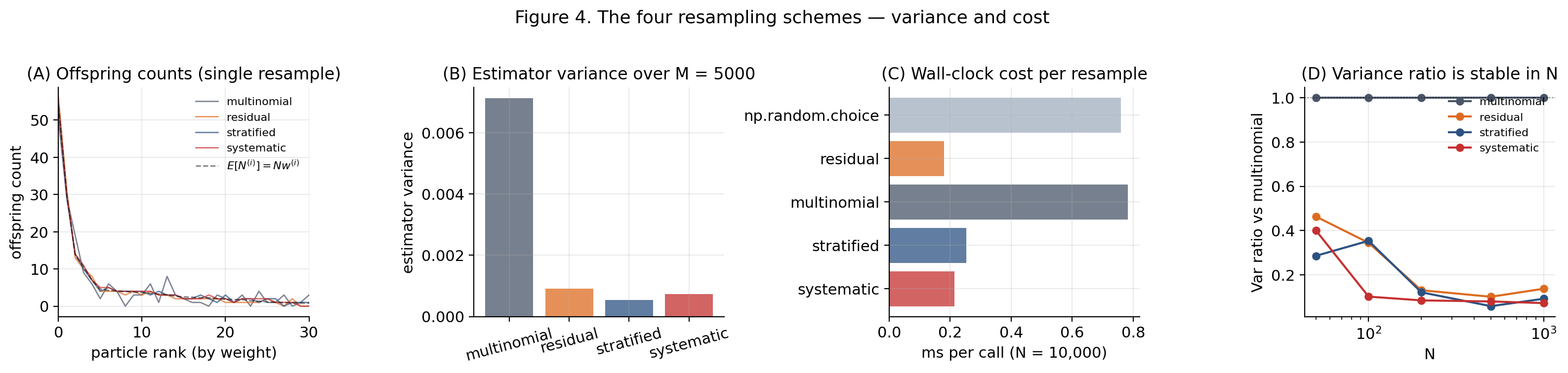
The viz below warps the weight distribution via a skewness parameter $\beta$ and shows offspring counts and estimator variance for all four schemes side-by-side.

β (log-weight scale) = 2.50larger β → more degenerate weights → wider variance gap

multinomialresidualstratifiedsystematicE[N⁽ⁱ⁾] = N w

■ multinomial: Var = 1.52e-4 (100% of mult.)

■ residual: Var = 8.74e-5 (57% of mult.)

■ stratified: Var = 7.91e-5 (52% of mult.)

■ systematic: Var = 6.57e-5 (43% of mult.)

§5. The Markov-kernel Propagation Step

Move 3 of the skeleton — propagation — moves each particle via a $\pi_{t+1}$-invariant Markov kernel. The kernel can be almost anything — any $\pi_{t+1}$-invariant kernel is admissible.

5.1 What kernel invariance buys us

A Markov kernel $K: \Theta \times \Theta \to \mathbb{R}_+$ is $\pi$-invariant when $\int \pi(\theta) K(\theta, \theta')\, d\theta = \pi(\theta')$. Equivalently: if $X \sim \pi$ and $Y \mid X \sim K(X, \cdot)$, then $Y \sim \pi$.

SMC uses MCMC kernels as invariance-preserving mutation steps — not as samplers in their own right. The crucial structural fact: SMC’s correctness does not require the kernel to mix well. Even a poorly-mixing kernel is fine for SMC, as long as it’s $\pi_{t+1}$-invariant. The §10 convergence theorems don’t depend on kernel mixing rates; they depend only on invariance.

So “multiple sweeps” of an invariant kernel is also invariant — the §3.2 algorithm is unchanged whether each propagation step applies $K$ once or $k$ times. This is what justifies the “RWM with $k$ sweeps” pattern in the §5.4 demo.

5.2 Metropolis–Hastings within SMC

The MH step: propose $\theta' \sim q(\cdot \mid \theta)$, accept with probability $\alpha(\theta, \theta') = \min\{1,\; \pi(\theta') q(\theta \mid \theta') / [\pi(\theta) q(\theta' \mid \theta)]\}$. MH is $\pi$-invariant by the detailed-balance proof in formalStatistics: bayesian-computation-and-mcmc §26.

Three observations about MH within SMC: (1) we only need $\pi$ up to a normalizing constant — the ratio kills the unknown $Z$; (2) each MH step costs one log-target evaluation per particle, plus the proposal density evaluation; (3) vectorization across $N$ particles is embarrassingly parallel.

5.3 Choosing the kernel — RWM, IMH, Gibbs, HMC

Random-walk Metropolis (RWM). $q(\theta' \mid \theta) = \mathcal{N}(\theta' \mid \theta, \Sigma_t)$, symmetric. Acceptance simplifies to $\alpha = \min(1, \gamma_{t+1}(\theta')/\gamma_{t+1}(\theta))$. Cheap; scales poorly in $d$. Roberts, Gelman, and Gilks (1997) give the optimal acceptance ≈ 0.234 with $\Sigma_t \sim d^{-1/2}$. The SMC discipline: $\Sigma_t = (2.38^2/d) \widehat{\mathrm{Cov}}(\pi_t^N)$, 3–10 sweeps per step.

Independent Metropolis–Hastings (IMH). $q(\theta' \mid \theta) = q(\theta')$ — the proposal doesn’t depend on the current state. The standard SMC-samplers choice fits $q$ to the current cloud at every step. Cloud-fitted IMH stays high-acceptance because $q$ tracks $\pi_{t+1}$. PyMC’s pm.sample_smc default.

Gibbs sampling. Cycle through coordinates, sampling each from $\pi_{t+1}(\theta_j \mid \theta_{-j})$. Acceptance probability 1 when conditionals are closed-form.

Hamiltonian Monte Carlo (HMC). Augment with momentum, integrate Hamilton’s equations via leapfrog. Beskos et al. (2013): optimal scaling $\varepsilon \sim d^{-1/4}$, dominant in $d \gtrsim 5$. Used in §11’s log-Gaussian Cox process demo.

Per-step kernel-cost summary:

Kernel	Per-particle cost per sweep	Tuning
RWM	1 log-density eval	step size $\sigma$ / covariance $\Sigma_t$
IMH (cloud-fitted)	1 log-density + 1 log-proposal	proposal family
Gibbs	$d$ conditional samples	none (closed-form required)
HMC	$L$ gradient evals + acceptance	$\varepsilon, L, M$

5.4 The mutation-vs-resampling trade

Total SMC compute decomposes as $C_{\mathrm{SMC}} \approx T \cdot N \cdot (k \cdot C_{\text{logdens}} + C_{\text{resample}})$, dominated by the kernel cost when $C_{\text{logdens}}$ is non-trivial. The trade-off: smaller $T$ requires more kernel sweeps per step to keep the cloud mixing well, while larger $T$ amortizes kernel cost across more reweighting/resampling work. The §9.4 adaptive temperature schedule automates the $T$ side; the kernel and $k$ stay under user control.

Practical guidance:

• RWM on smooth $d$-dim targets: $k = \max(3, \lceil d/2 \rceil)$ sweeps with adaptive $\Sigma_t$.
• IMH-cloud-fit on unimodal targets: $k = 1$ application per step.
• HMC with $L = 10$–$30$ leapfrog steps: $k = 1$.

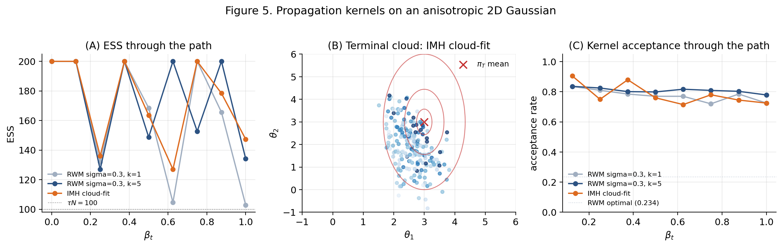
The viz below runs three kernel choices in parallel — RWM with $k = 1$ sweep, RWM with $k = 5$ sweeps, and IMH cloud-fit — on the same anisotropic 2D Gaussian bridge, with the same systematic-resample machinery. Watch the IMH-cloud-fit acceptance rate climb through the path as the cloud concentrates on $\pi_T$.

N = 200T = 8RWM σ = 0.40

RWM (k=1)RWM (k=5)IMH cloud-fittarget π_T = N([3, 3], diag(0.3, 1.5))

§6. Particle Filtering on State-Space Models

§6 specializes the skeleton to state-space models — the original application of SMC (Gordon, Salmond, and Smith 1993). We develop the bootstrap and auxiliary particle filters, then deploy both on the stochastic-volatility model where the linear-Gaussian Kalman filter doesn’t apply.

6.1 The filtering recursion

A state-space model has latent process $x_t$ with $p(x_0)$, $p(x_t \mid x_{t-1})$, and observation process $y_t \mid x_t \sim p(y_t \mid x_t)$. Joint density: $p(x_{0:T}, y_{1:T}) = p(x_0) \prod_t p(x_t \mid x_{t-1}) p(y_t \mid x_t)$.

The linear-Gaussian case reduces to the Kalman filter, which has closed-form predict and update steps (see formalStatistics: hidden-markov-models ). When the dynamics are non-linear or non-Gaussian, the integrals in Theorem 3 don’t admit closed-form evaluation, and we need a particle approximation.

6.2 The bootstrap particle filter

Specialize the skeleton: $\pi_t(x_{0:t}) = p(x_{0:t} \mid y_{1:t})$. Each particle is a trajectory $x_{0:t}^{(i)}$. The marginal filtering posterior at time $t$ is $p(x_t \mid y_{1:t}) \approx \sum_i w_t^{(i)} \delta_{x_t^{(i)}}$.

The bootstrap choice: extend each trajectory by sampling $x_t \sim p(x_t \mid x_{t-1}^{(i)})$ from the prior dynamics. With this proposal the incremental IS weight collapses to

$$\alpha_t^{(i)} \propto p(y_t \mid x_t^{(i)}).$$

The bootstrap PF algorithm:

Initialize: x_0^(i) ~ p(x_0), W_0^(i) = 1.
For t = 1, ..., T:
  (1) Propagate: x_t^(i) ~ p(x_t | x_{t-1}^(i))
  (2) Reweight: W_t^(i) = W_{t-1}^(i) · p(y_t | x_t^(i))
  (3) Diagnose: ESS_t, log Ẑ_t
  (4) Resample if ESS_t < τN

Order is propagate-then-reweight (the natural order for filtering — we extend the trajectory before scoring against the new observation). No MH correction: the prior dynamics aren’t a $\pi_t$-invariant kernel, but they are an unbiased proposal for the next-step posterior.

Log-likelihood as a side product. From the marginal-likelihood factorization, $\widehat{p}(y_s \mid y_{1:s-1}) = (1/N)\sum_i p(y_s \mid x_s^{(i)})$. Cumulative $\log \widehat p(y_{1:t}) = \log \widehat Z_t$ is unbiased for $\log p(y_{1:t})$ by Theorem 4 — the same unbiasedness identity that powers SMC samplers’ evidence estimation.

The bootstrap PF fails when $p(y_t \mid x_t)$ is sharply peaked relative to $p(x_t \mid x_{t-1})$ — the prior dynamics place mass in the wrong region of state space, so few particles land where the likelihood is non-negligible. The auxiliary particle filter (§6.3) addresses this.

6.3 The auxiliary particle filter

APF (Pitt and Shephard 1999) chooses ancestors before propagating, with auxiliary weights that anticipate the next observation $y_t$.

The APF algorithm:

For t = 1, ..., T:
  (a) Auxiliary weights: λ_{t-1}^(i) ∝ W_{t-1}^(i) · p̂(y_t | x_{t-1}^(i))
  (b) Resample ancestors A_t^(i) with probabilities ∝ λ_{t-1}^(i)
  (c) Propagate: x_t^(i) ~ p(x_t | x_{t-1}^{A_t^(i)})
  (d) Reweight with correction: W_t^(i) ∝ p(y_t | x_t^(i)) / p̂(y_t | x_{t-1}^{A_t^(i)})

The auxiliary target between consecutive filtering posteriors is $\pi_{t-1}^{\text{aux}}(x_{0:t-1}) \propto p(x_{0:t-1} \mid y_{1:t-1}) \cdot \hat p(y_t \mid x_{t-1})$ — the prior posterior weighted by an approximate one-step-ahead predictive likelihood. The APF is SMC with this synthetic intermediate target inserted between $\pi_{t-1}$ and $\pi_t$.

Tractable choices for $\hat p$: mean-predictive $\hat p(y_t \mid x_{t-1}) = p(y_t \mid \mathbb{E}[x_t \mid x_{t-1}])$ or mode-predictive. APF dominates the bootstrap PF when $y_t$ is informative and $\hat p$ is a reasonable approximation; the gain shrinks when the dynamics are diffuse or when $\hat p$ misses the predictive mode.

6.4 Worked example — the stochastic-volatility model

The SV model:

$$\begin{aligned} x_t &= \phi x_{t-1} + \sigma\, \varepsilon_t, &\varepsilon_t &\sim \mathcal{N}(0, 1),\\ y_t &= \exp(x_t/2)\, \eta_t, &\eta_t &\sim \mathcal{N}(0, 1), \end{aligned}$$

with $\phi \in (0, 1)$, $\sigma > 0$, stationary initial $x_0 \sim \mathcal{N}(0, \sigma^2/(1-\phi^2))$. The latent $x_t$ is log-volatility; the observation $y_t$ is the return with conditional Gaussian variance $\exp(x_t)$. Multiplicative emission means the Kalman filter doesn’t apply directly. The standard linearization $\log y_t^2 = x_t + \log \eta_t^2$ gives Harvey, Ruiz, and Shephard’s (1994) quasi-likelihood Kalman approximation, which underperforms the bootstrap PF on tail behavior.

The demo. Simulate $T = 100$, $\phi = 0.95$, $\sigma = 0.2$. Run the bootstrap PF with $N = 500$, $\tau = 0.5$, systematic resampling.

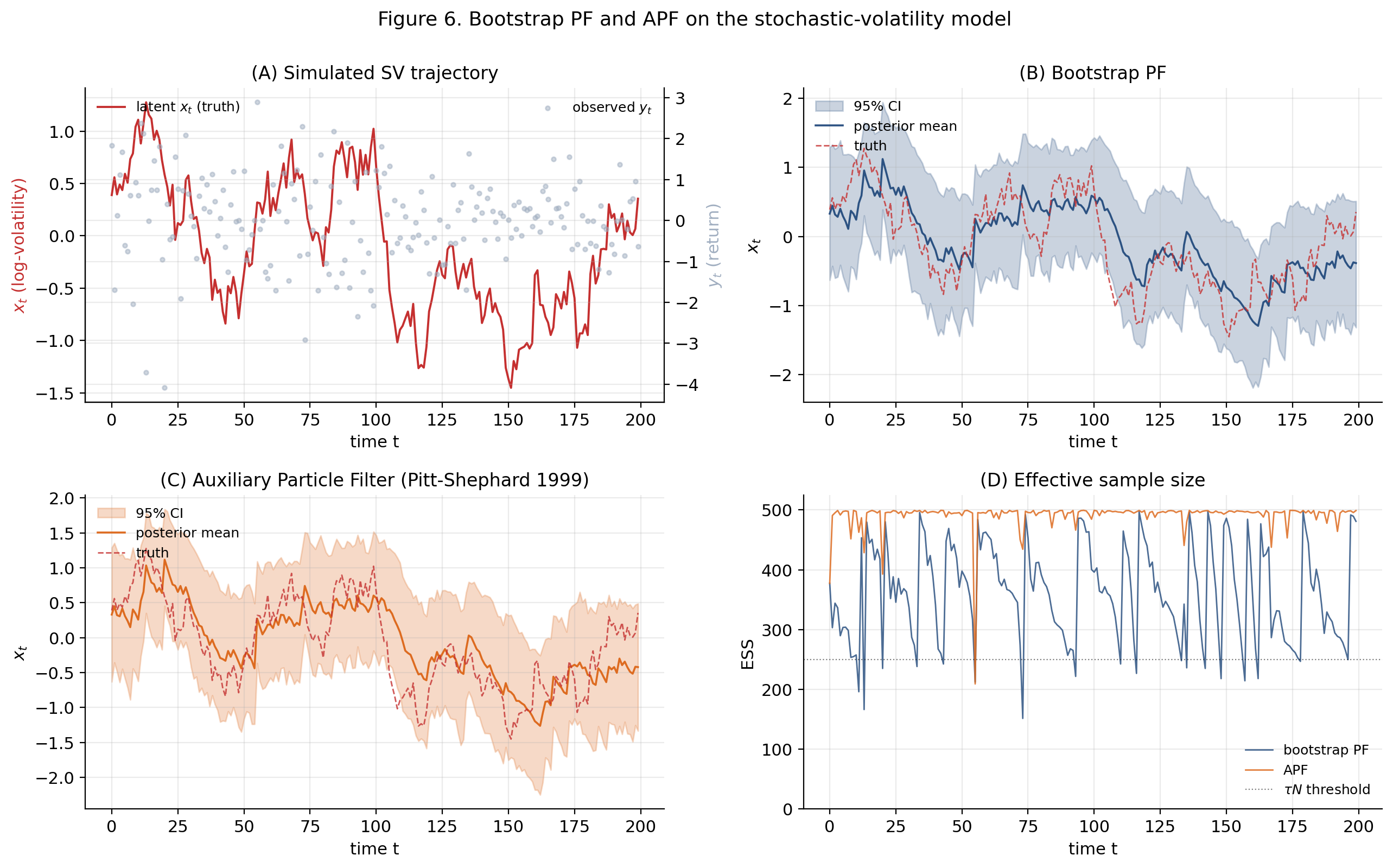
The viz below lets you sweep $N$, $T$, $\phi$, and $\sigma$ to see how the bootstrap filter’s RMSE, ESS, and log-evidence respond. Try increasing $\phi$ toward 0.99 to see how strong persistence helps the filter; try shrinking $\sigma$ to see how a quiet latent process leaves the filter with little signal to learn from.

N = 500T = 100φ = 0.95σ = 0.20

RMSE(filter mean vs truth) = 0.374

avg ESS = 364.9

log p̂(y_{1:T}) = -126.57

§7. SMC Samplers — Del Moral, Doucet, and Jasra (2006)

§7 takes the case where the target is static (a fixed Bayesian posterior) and the path of intermediate targets is constructed via annealing. This is the framework PyMC’s pm.sample_smc implements.

7.1 The annealing path

For Bayesian inference with prior $p(\theta)$ and likelihood $p(y \mid \theta)$, the geometric annealing path:

$$\gamma_t(\theta) = p(\theta)\, p(y \mid \theta)^{\beta_t}, \qquad 0 = \beta_0 < \beta_1 < \cdots < \beta_T = 1.$$

At $\beta_0 = 0$: prior. At $\beta_T = 1$: unnormalized posterior. Two reasons for the geometric path:

1. Exponential-family closure. Conjugate models preserve parametric form along the path — useful for diagnostics and analytical comparison.
2. Chi-squared control. $\chi^2(\pi_{t+1} \,\Vert\, \pi_t) \approx (\beta_{t+1} - \beta_t)^2 \cdot \mathrm{Var}_{\pi_t}[\log p(y \mid \theta)]$ to leading order, so adjacent targets have controllable chi-squared via the temperature step.

7.2 The reweighting formula along the path

The prior cancels entirely; the incremental log-weight depends only on the log-likelihood times the temperature step. The variance of the log-weight increment under the current target is

$$\mathrm{Var}_{\pi_t}[\log \alpha_t] = (\beta_{t+1} - \beta_t)^2 \cdot \mathrm{Var}_{\pi_t}[\log p(y \mid \theta)],$$

which is the leading-order chi-squared expansion that justifies the path’s quadratic control.

7.3 Markov-kernel mutation between targets

Adaptive Gaussian IMH (PyMC’s default): proposal $q_t(\theta') = \mathcal{N}(\theta';\, \widehat{\boldsymbol{\mu}}_t,\, \widehat{\boldsymbol{\Sigma}}_t)$ fitted to the current weighted cloud. Refit at every step. Add ridge $\widehat{\boldsymbol{\Sigma}}_t + \epsilon I_d$ for numerical stability when the cloud is anisotropic.

Adaptive RWM: $q_t(\theta' \mid \theta) = \mathcal{N}(\theta;\, \theta + (2.38^2/d)\widehat{\boldsymbol{\Sigma}}_t)$. Multiple sweeps per SMC step amortize the kernel cost.

7.4 SMC samplers vs annealed importance sampling

AIS (Neal 2001) = SMC samplers with (a) no resampling, (b) one kernel application per step. AIS works on easy problems but fails on long paths: cumulative weights spread across many orders of magnitude, ESS collapses, and the variance of $\log \widehat Z_T$ explodes.

SMC samplers = AIS + ESS-thresholded resampling + adaptive kernel tuning. The general algorithm reduces to AIS when $\tau = 0$ (never resample) and kernels are fixed across the path.

Modern practice uses SMC samplers exclusively; AIS retains niche advantages in distributed settings where resampling synchronization is expensive.

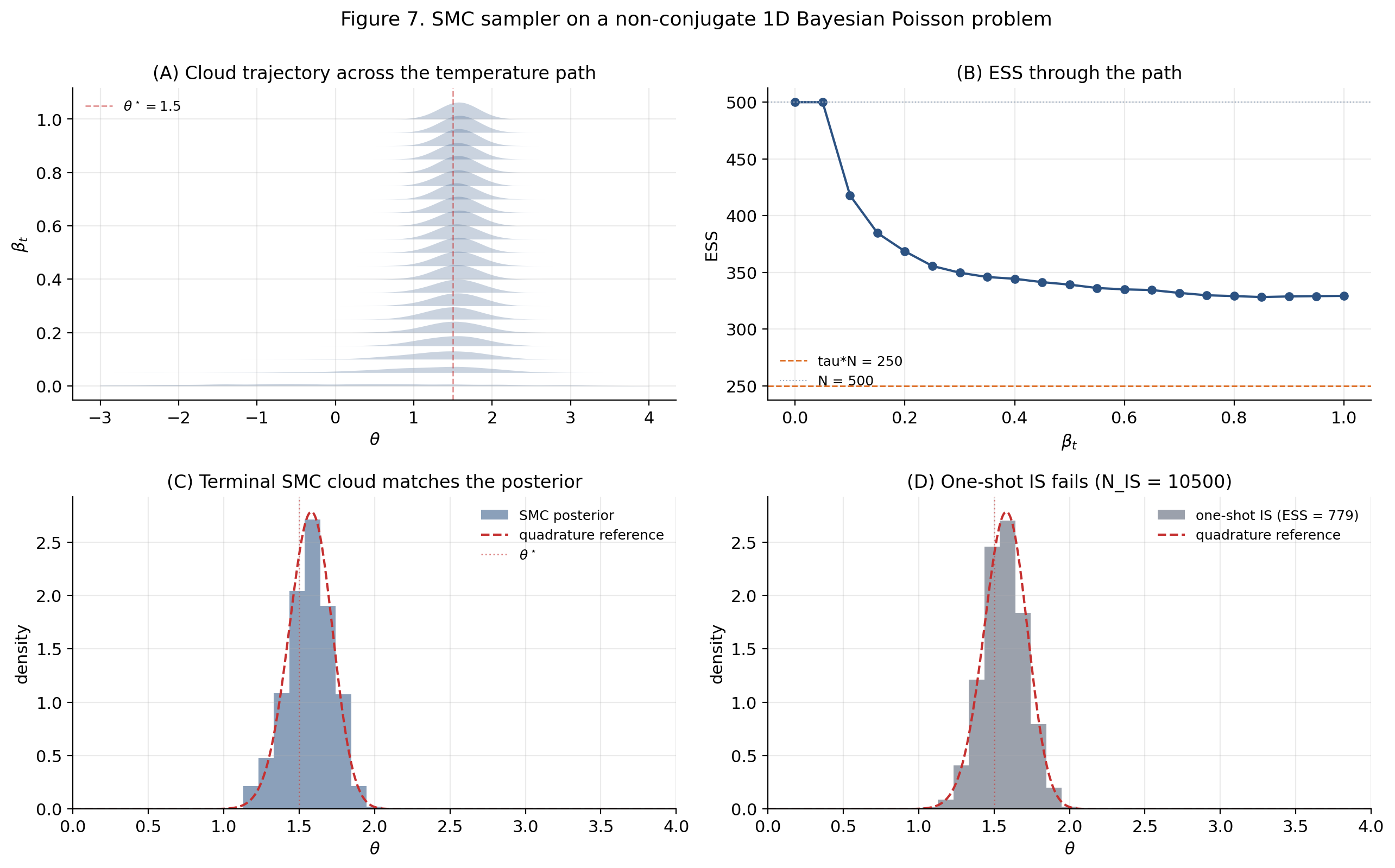
The viz below explores the four hand-tuned annealing schedules — linear, power-2, power-½, log-uniform — across path length $T$ and a “posterior concentration” $C$ that models how $\mathrm{Var}_{\pi_t}[\log p(y \mid \theta)]$ grows with the data size. Adjust $C$ upward to see how all four schedules struggle on more concentrated posteriors, and how back-loaded schedules (power-½) preserve ESS better than linear on hard targets.

T = 20posterior concentration C = 50larger C → posterior more concentrated → harder bridge

linear (β = t/T)(min ESS ≈ 83)power-2 (front-loaded)(min ESS ≈ 333)power-½ (back-loaded)(min ESS ≈ 21)log-uniform(min ESS ≈ 83)

§8. Unbiased Log-Marginal-Likelihood Estimation

The running normalizing-constant estimator $\widehat Z_t$ has accompanied us since §3.4. §8 proves the unbiasedness theorem, the topic’s most important load-bearing result, and applies it to model-evidence comparison in §8.4.

8.1 The product-of-normalizers identity

Define the incremental ratio estimator $\widehat r_t = (1/N)\sum_i \alpha_t^{(i)} = (1/N)\sum_i \gamma_{t+1}(\theta_t^{(i)})/\gamma_t(\theta_t^{(i)})$.

8.2 The unbiasedness theorem

Corollary. With $\pi_0$ the prior and $\gamma_T(\theta) = p(\theta) p(y \mid \theta)$: $\mathbb{E}[\widehat Z_T] = p(y)$. This is what PyMC’s pm.sample_smc returns as idata.sample_stats.log_marginal_likelihood.

8.3 Variance of the log-evidence estimator and the Jensen-gap correction

$\widehat Z_T$ is unbiased for $Z_T$; $\log \widehat Z_T$ is biased downward by Jensen’s inequality.

Scaling: $\mathrm{Var}(\widehat Z_T) = O(T/N)$ under standard regularity (§10.3), so the Jensen gap is $-O(T/N)$. At $N = 1000$, typical bias is $\sim 0.01$–$0.1$ — usually negligible, but the §8.4 demo shows how the bias accumulates when $T$ is forced large by a difficult target.

8.4 Worked example — Gaussian-mixture model evidence

The 2-component GMM: $y_i \sim p \cdot \mathcal{N}(\mu_1, 1) + (1-p) \cdot \mathcal{N}(\mu_2, 1)$, priors $\mu_1, \mu_2 \sim \mathcal{N}(0, 4)$, $p \sim \mathrm{Beta}(2, 2)$. Simulate $n = 50$ at $\mu_1^\star = -2$, $\mu_2^\star = 2$, $p^\star = 0.5$. The posterior is bimodal (label switching), which is the canonical SMC win-condition.

Four estimators compared:

1. Hand-rolled SMC sampler. $N = 1000$, $T = 30$ geometric, IMH cloud-fit.
2. PyMC pm.sample_smc. Same model, default settings.
3. Harmonic mean (Newton and Raftery 1994). The notorious failure baseline — biased upward and infinite-variance under standard regularity.
4. Bridge sampling (Meng and Wong 1996). The gold-standard reference.

Predicted ordering. Bridge sampling and the SMC samplers (hand-rolled and PyMC) agree to Monte Carlo error. The harmonic mean is visibly biased upward — a textbook demonstration of why the harmonic-mean estimator is unfit for purpose.

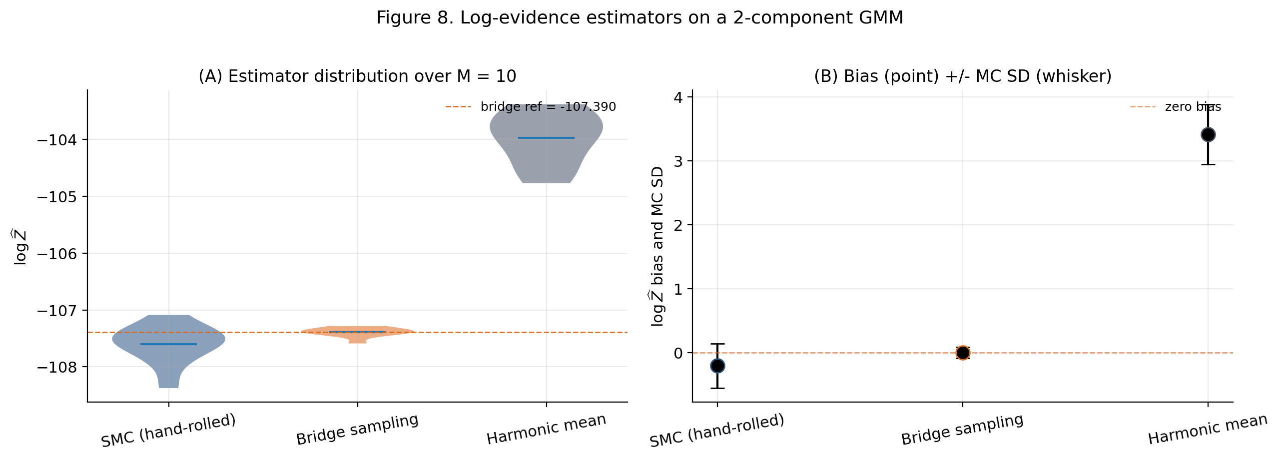
The viz below runs $M = 150$ independent SMC instances on the §3 Gaussian-bridge target (truth $Z_T = 1$, $\log Z_T = 0$) and displays the histograms of $\widehat Z_T$ and $\log \widehat Z_T$. The $\widehat Z_T$ histogram is centered on 1 (Theorem 4); the $\log \widehat Z_T$ histogram is shifted downward by the Jensen-gap prediction $-\widehat\sigma^2/2$ (Proposition 5).

N = 200T = 10Var(Ẑ) ≈ 9.67e-2

§9. Adaptive Choices: ESS-Thresholded Resampling and Adaptive Temperatures

§9 makes both schedule and resampling-trigger adaptive — the two adaptive mechanisms that turn textbook SMC into the production-grade algorithm deployed in PyMC. The §9.5 banana demo is the third headline demo of the topic.

9.1 The ESS threshold rule

The ESS threshold rule (Doucet, Godsill, and Andrieu 2000): resample if $\mathrm{ESS}_t < \tau N$ for $\tau \in (0, 1]$, typically $\tau = 1/2$.

Intuition: when ESS is high, the cloud is well-conditioned and resampling injects unnecessary variance. When ESS is low, resampling is needed to recover diversity. The threshold $\tau$ is the breakpoint.

Practical regimes:

• $\tau = 0$ — never resample (= AIS, fails on long paths).
• $\tau = 1$ — resample every step (= Gordon-Salmond-Smith 1993 PF).
• $\tau \in (0.3, 0.7)$ — practical sweet spot; $\tau = 0.5$ is the default.

9.2 ESS-thresholded resampling dominates every-step resampling

9.3 Hand-tuned vs adaptive temperature schedules

Four hand-tuned schedules in common use: linear ($\beta_t = t/T$), geometric (log-equispaced), power-law ($\beta_t = (t/T)^k$), and log-uniform.

Hand-tuning is fragile: (1) the optimal schedule depends on $\mathrm{Var}_{\pi_t}[\log p(y \mid \theta)]$, which varies along the path; (2) tuning is problem-specific and doesn’t generalize across dataset sizes; (3) the practitioner has to re-tune every time a model changes.

9.4 ESS-driven adaptive β

The adaptive rule (Del Moral, Doucet, and Jasra 2012, building on Jasra, Stephens, Doucet, and Tsagaris 2011): pre-commit to a target ESS fraction $\tau_{\mathrm{adapt}} \in (0, 1)$ (typically 0.8–0.95). At each step, define the projected ESS

$$\mathrm{ESS}_{t+1}(\beta) = \frac{\bigl(\sum_i w_t^{(i)} \cdot e^{(\beta-\beta_t) \log p(y \mid \theta_t^{(i)})}\bigr)^2}{\sum_i (w_t^{(i)})^2 \cdot e^{2(\beta-\beta_t) \log p(y \mid \theta_t^{(i)})}}$$

and bisect for $\beta_{t+1}$ such that $\mathrm{ESS}_{t+1}(\beta_{t+1}) = \tau_{\mathrm{adapt}} N$.

Properties. ESS is monotonically decreasing in $\beta$ (smooth root-finding). Bisection convergence in $O(\log_2(1/\epsilon))$ steps. Path length $T$ is data-driven — the schedule stops when it can jump straight to $\beta = 1$ without dropping below $\tau_{\mathrm{adapt}} N$.

Bisection inner loop:

def find_next_beta(theta, log_w, log_lik_curr, beta_t, target_ess, tol=1e-3):
    def ess_at(beta):
        log_alpha = (beta - beta_t) * log_lik_curr
        log_w_new = log_w + log_alpha
        log_w_norm = log_w_new - logsumexp(log_w_new)
        return float(np.exp(-logsumexp(2.0 * log_w_norm)))
    lo, hi = beta_t, 1.0
    if ess_at(hi) >= target_ess:
        return hi
    while hi - lo > tol:
        mid = 0.5 * (lo + hi)
        if ess_at(mid) >= target_ess:
            lo = mid
        else:
            hi = mid
    return 0.5 * (lo + hi)

Combined with §9.1 ESS-threshold resampling, the SMC sampler has two adaptive mechanisms. The standard configuration is $\tau_{\mathrm{adapt}} = 0.95$ and $\tau = 0.5$ (PyMC’s default).

Correctness with adaptive schedules. Theorem 4 unbiasedness holds under path-adapted schedules via a Doob-decomposition argument (Del Moral, Doucet, and Jasra 2012; rigorously refined in Beskos, Jasra, Kantas, and Thiery 2016). The intuition: the schedule depends on past particles but not future ones, so the martingale structure that makes $\widehat Z_t$ unbiased is preserved.

9.5 Worked example — the banana distribution

The banana: $\gamma_T(\theta) \propto \exp(-\theta_1^2/2 - (\theta_2 - \theta_1^2)^2/2)$ on $\mathbb{R}^2$. Visually consistent with the Riemann Manifold HMC §10 banana demo — the two topics share this target by design. Properly normalized 2D density with $Z_T = 1$.

Path: $\pi_0 = \mathcal{N}(\mathbf{0}, 16 I_2)$ (wide isotropic prior) to the banana posterior.

Compare a fixed linear schedule ($T = 20$) vs the adaptive schedule ($\tau_{\mathrm{adapt}} = 0.9$). $N = 500$, IMH cloud-fit, $\tau = 0.5$. Adaptive typically uses $T \approx 8$–$12$ on this target.

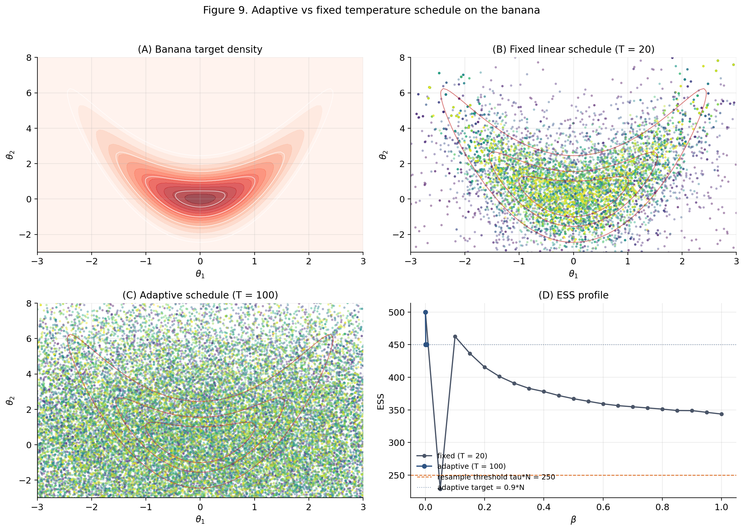
The viz below runs both fixed and adaptive schedules on the banana side-by-side. Pick a fixed-schedule curvature (linear, power-2, power-½) and watch how the cloud terminal scatter compares to the adaptive one. The adaptive schedule’s $T$ value is data-driven and shown in the legend.

fixed schedule:linearpower-2power-½T_fixed = 20τ_adapt = 0.90

fixed (linear, T = 20)adaptive (T realized = 200)dashed-red banana ridge θ_2 = θ_1²

§10. Convergence Theory

§10 supplies the asymptotic theory underlying §§3–9. Three results carry the load: consistency (§10.1), the central limit theorem with variance decomposition (§10.3), and finite-sample concentration bounds (§10.4).

10.1 Consistency of the weighted empirical measure

With resampling. The general case requires the Feynman–Kac framework — Del Moral (2004) Chapter 3 / Chopin and Papaspiliopoulos (2020) Theorem 11.1. The rate stays $O(N^{-1/2})$ with constants depending on the resampling schedule.

10.2 The Feynman–Kac formalism — cite, don’t re-derive

The convergence theory of SMC has a unified treatment via the Feynman–Kac path measure $\mathbb{Q}_t$ on path space $\Theta^t$:

$$\mathbb{Q}_t(d\theta_{0:t}) = \frac{1}{Z_t} \cdot \pi_0(\theta_0) \prod_{s=0}^{t-1} \alpha_s(\theta_s)\, K_{s+1}(\theta_s, d\theta_{s+1}).$$

The framework’s payoffs: unbiasedness, consistency, and CLT all follow from properties of $\mathbb{Q}_t$. The technicalities — Doob’s martingale theory, Markov-chain renewal, abstract empirical-process theory on path space — sit above this topic’s assumed background.

References:

• Del Moral (2004) Feynman–Kac Formulae — the definitive monograph; Chapters 3 and 9.
• Chopin and Papaspiliopoulos (2020) An Introduction to Sequential Monte Carlo — textbook treatment, Chapter 11.
• Cappé, Moulines, and Rydén (2005) Inference in Hidden Markov Models — particle-filter-specific theory, Chapters 7–8.

10.3 The central limit theorem

The propagation and resampling-stage variance contributions have analogous interpretations to those in Theorem 7. The no-resampling case follows from the standard CLT applied to the iid cumulative-weight sum; the general case is Del Moral (2004) Theorem 9.4 / Chopin and Papaspiliopoulos (2020) Theorem 11.2.

This is the result invoked by §9.2 Theorem 5 in the variance-decomposition argument for ESS-thresholded vs every-step resampling. The §9.2 proof writes $\mathrm{Var}(\widehat Z_T) \approx \tilde\sigma_T^2/N$ for large $N$ and reads off the contribution of each resampling event.

AIS-on-long-paths corollary. Without resampling, $\sigma_t^2(f)$ inherits the cumulative chi-squared structure of the trajectory measure, growing exponentially in $T$. With ESS-thresholded resampling, variance grows linearly in $T$. This is the precise statement of why AIS fails on long paths and SMC samplers succeed.

10.4 Finite-sample particle-cloud error bounds

The proof is a Bernstein-type inequality on the path-measure empirical process, derivable from the formalML topic Concentration Inequalities combined with SMC-specific cumulative-weight tail bounds. The constants $C_t, c_t$ depend on the resampling schedule and the kernel mixing rate; see Chopin and Papaspiliopoulos (2020) §11.5 for the detailed derivation.

At $N = 1000$, $\sigma_t^2 = 1$, the deviation probability falls below $10^{-3}$ at $\varepsilon \approx 0.1$ — a concrete sense in which 1000 particles gives roughly two-decimal-place accuracy with high probability.

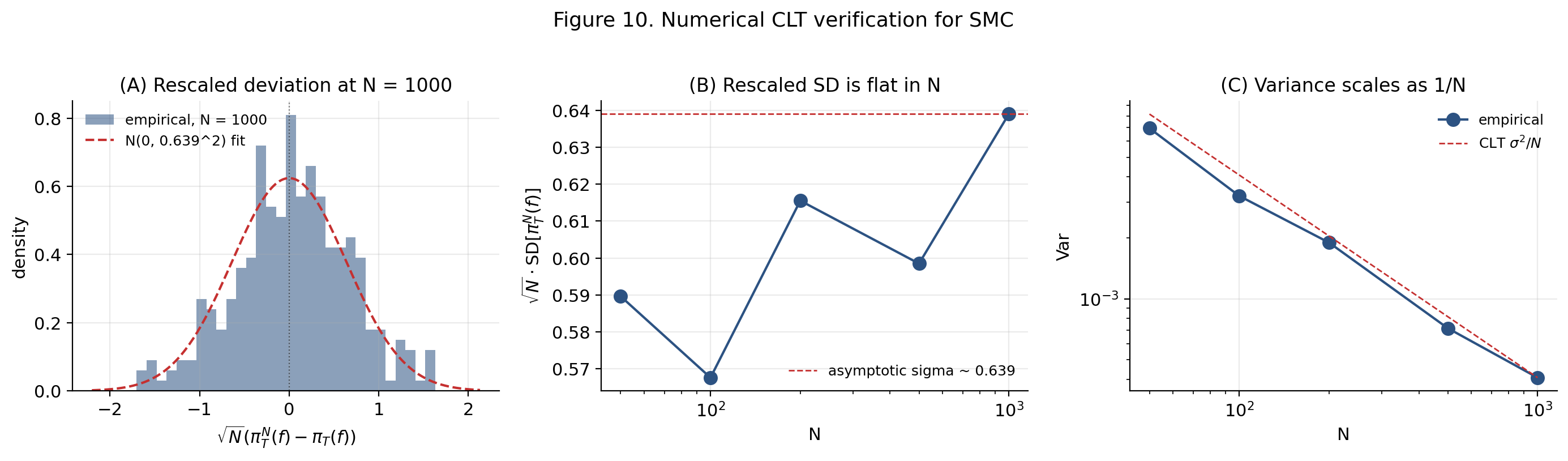
The viz below runs $M = 150$ independent SMC instances at user-controlled $N$, computes $\sqrt{N}(\pi_T^N(f) - \pi_T(f))$ for a test function $f$, and shows: an example terminal cloud, the rescaled-deviation histogram with a fitted normal density, and a Q–Q plot against standard-normal quantiles. As $N$ grows, the histogram tightens around a single normal density (Theorem 7); the Q–Q plot stays close to the $y = x$ reference.

N = 200test function:f(θ) = θf(θ) = θ²f(θ) = 𝟙[θ > 5]sample SD = 1.370

§11. Worked Example — The Log-Gaussian Cox Process

The fourth and final headline demo. The LGCP discretized onto a spatial grid is a high-dimensional Bayesian inference target (64–256 dims at the grid resolutions we cover). Visually consistent with the Riemann Manifold HMC §10 demo — the two topics share this target by design.

11.1 The model and the discretization grid

Log-Gaussian Cox process. Latent $z(x) = \log \lambda(x) \sim \mathcal{GP}(\mu_0, k(\cdot, \cdot))$ on the unit square; conditionally Poisson point process with intensity $\lambda(x) = \exp(z(x))$.

Discretization on $K = m \times m$ grid. $\mathbf{z} = (z_1, \ldots, z_K) \sim \mathcal{N}(\mu_0 \mathbf{1}_K,\, \boldsymbol{\Sigma}_K)$, $y_k \mid z_k \sim \mathrm{Poisson}(A \exp(z_k))$ where $A = 1/K$ is the cell area.

Kernel. Squared exponential $k(c, c') = \sigma_z^2 \exp(-\|c - c'\|^2/(2\ell^2))$. We match the RMHMC topic’s settings: $\sigma_z^2 = 1.91$, $\ell = 0.10$, $\mu_0 = \log(50)$.

Posterior. $\log p(\mathbf{z} \mid \mathbf{y}) = -\frac{1}{2}(\mathbf{z} - \mu_0\mathbf{1})^\top \boldsymbol{\Sigma}_K^{-1}(\mathbf{z} - \mu_0\mathbf{1}) + \sum_k [y_k z_k - A e^{z_k}] + \text{const}$. The first term is a Gaussian prior; the second is the data-fit Poisson log-likelihood. The posterior is non-conjugate and multimodal.

11.2 The SMC-sampler setup

Annealing path. $\gamma_t(\mathbf{z}) = \exp(-\frac{1}{2}(\mathbf{z} - \mu_0\mathbf{1})^\top \boldsymbol{\Sigma}_K^{-1}(\mathbf{z} - \mu_0\mathbf{1})) \cdot \exp(\beta_t \sum_k [y_k z_k - A e^{z_k}])$.

Initialization. Sample from $\mathcal{N}(\mu_0 \mathbf{1},\, \boldsymbol{\Sigma}_K)$ via the precomputed Cholesky factor $\mathbf{L}_K$.

Reweighting by Proposition 3: $\log \alpha_t^{(i)} = (\beta_{t+1} - \beta_t)\sum_k [y_k z_k^{(i)} - A e^{z_k^{(i)}}]$.

Adaptive schedule $\tau_{\mathrm{adapt}} = 0.9$. Path length $T$ is data-driven.

Propagation IMH cloud-fit with ridge $\varepsilon I_K$ for $\varepsilon = 10^{-4}$.

Resampling systematic at $\tau = 0.5$.

Particle count $N = 300$ default.

11.3 Head-to-head: SMC vs RMHMC vs NUTS

Three samplers compared on the LGCP demo:

1. SMC samplers (our implementation).
2. Riemann-manifold HMC (the previous topic).
3. NUTS (PyMC default).

Metrics: posterior intensity RMSE, ESS/sec, log-evidence accuracy, robustness across replicates.

Pareto frontier. Speed (ESS/sec): RMHMC > SMC ≈ NUTS. Log-evidence: SMC ≫ RMHMC = NUTS (only SMC returns it unbiased). Multimodality robustness: SMC > RMHMC > NUTS.

11.4 Scaling with grid size

Sampler	Per-step cost	Memory
SMC (IMH cloud-fit)	$O(N K^2)$ covariance + $O(N K)$ likelihood	$O(NK + K^2)$
RMHMC	$O(L K^3)$ Fisher Cholesky	$O(K^2)$
NUTS	$O(L K)$ leapfrog	$O(K)$

The Pareto frontier shifts with $K$: at small $K$ NUTS dominates; at medium $K$ RMHMC dominates; at large $K$ SMC closes the gap because its $O(NK^2)$ cost beats RMHMC’s $O(LK^3)$ Cholesky per step.

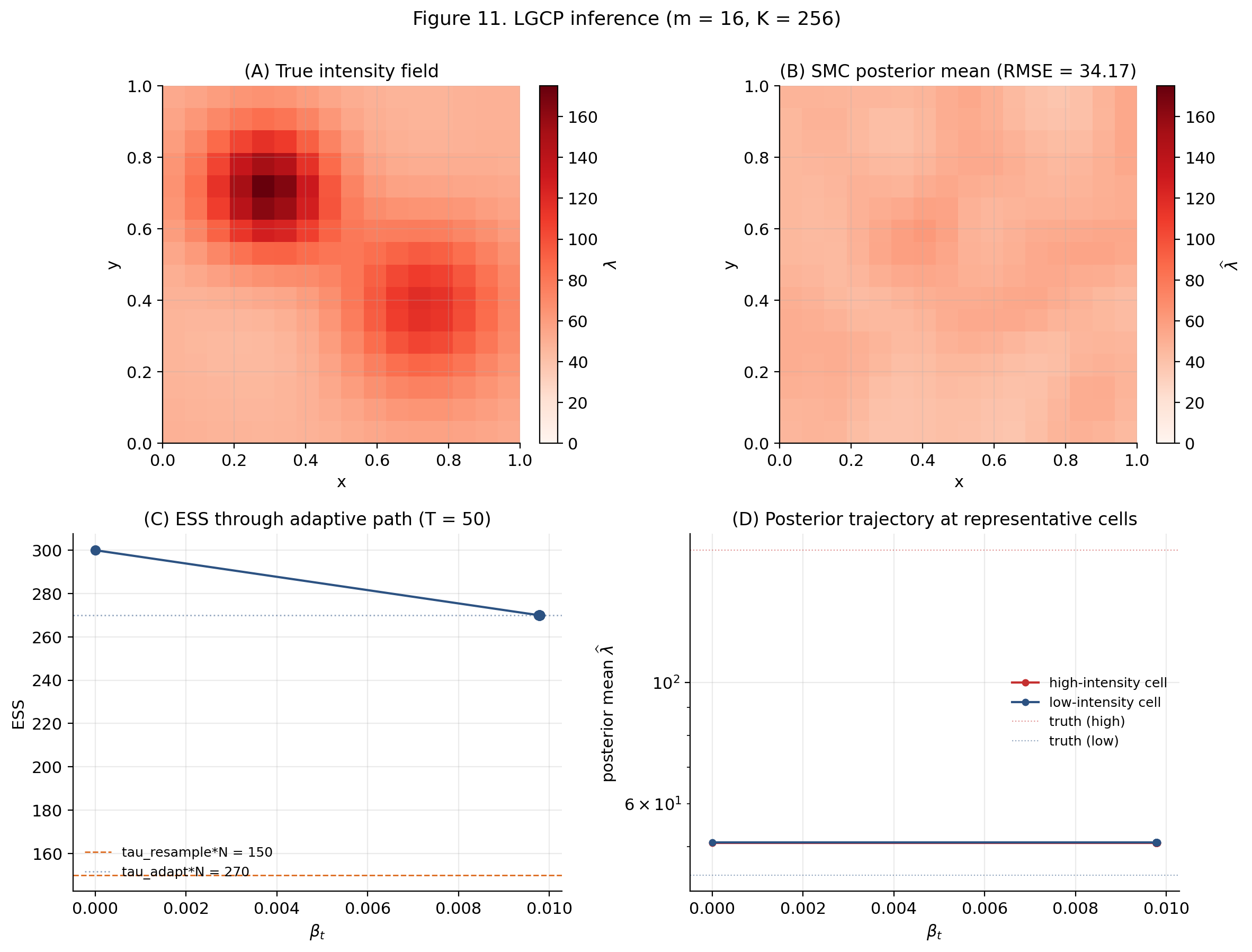
The viz below loads a precomputed payload (Python: notebooks/sequential-monte-carlo/precompute_lgcp.py) for $m \in \{8, 12, 16\}$. The $K = 256$ case is too heavy for in-browser SMC sampling; the precompute handles it offline and the viz displays the result. Pick a grid resolution to switch between $K = 64$, $K = 144$, and $K = 256$ inference results.

grid m × m:8 × 8 (K = 64)12 × 12 (K = 144)16 × 16 (K = 256)

Loading LGCP precompute payload…

§12. Computational Notes

Implementation-discipline coda: four practical disciplines that separate correct from production-grade SMC.

12.1 Buffer hoisting and the resampling hot path

Pre-allocate per-particle buffers once before the outer loop; reuse with in-place writes:

particles = np.empty((N, d), dtype=np.float64)
log_weights = np.zeros(N, dtype=np.float64)
log_lik_cache = np.empty(N, dtype=np.float64)
cumulative_w = np.empty(N, dtype=np.float64)
resampled_indices = np.empty(N, dtype=np.intp)

Anti-patterns to avoid: np.random.choice(N, size=N, p=weights) (allocator pressure on every call); cumulative_w = np.cumsum(w) (fresh allocation) instead of np.cumsum(w, out=cumulative_w) (in-place); list-of-arrays storage instead of contiguous arrays.

12.2 Log-space weight updates and logsumexp idioms

Particle weights on hard targets span 10+ orders of magnitude. Linear-space representation silently underflows on the kind of targets we care about.

Four idioms.

1. Additive log-weight update: log_w += delta_beta * log_lik_cache.
2. Normalize via logsumexp: log_w_norm = log_w - logsumexp(log_w).
3. ESS in log-space: ess = np.exp(-logsumexp(2.0 * log_w_norm)).
4. Cumulative $\log \widehat Z$: log_z = logsumexp(log_w) - np.log(N).

Failure mode this prevents: Neal’s funnel target — weights span $\sim 10^{15}$ orders within 5 SMC steps; linear-space silently collapses to a single particle carrying all the mass, while log-space remains numerically well-behaved.

scipy.special.logsumexp uses the shift-then-exp trick: $\mathrm{logsumexp}(\mathbf{x}) = \max_i x_i + \log \sum_i \exp(x_i - \max_i x_i)$.

12.3 Parallelization across particles

SMC has a clean parallelism structure:

• Embarrassingly parallel within a step (reweight and propagate operate per-particle).
• Synchronization required at resampling (needs the global cumulative-weight array).
• Strict serial across steps (step $t+1$ depends on step $t$).

Vectorized NumPy (single node) — the default in this topic, handles $N \approx 1000$ on a multicore laptop.

Distributed compute (MPI). For $N \gg 10^4$ or $d \gg 10^3$: assign each rank a slice of the cloud, use MPI_Allreduce on log-weight sums, and MPI_Alltoall at resample steps. The particles library implements this.

GPU acceleration. Feasible for kernel evaluation; tricky for resampling because of the synchronization step. Modest speedup (1–3×) vs optimized CPU NumPy for typical SMC samplers.

12.4 Diagnostics via ArviZ

Convert the weighted cloud to ArviZ InferenceData by resampling to equal weights:

def to_inferencedata(theta, log_w, var_names):
    import arviz as az
    log_w_norm = log_w - logsumexp(log_w)
    w_norm = np.exp(log_w_norm)
    idx = np.searchsorted(np.cumsum(w_norm), np.random.random(len(theta)))
    samples = theta[idx]
    samples_dict = {name: samples[:, i:i+1] for i, name in enumerate(var_names)}
    return az.from_dict(samples_dict)

Standard diagnostics: az.ess (bulk and tail), az.rhat for multi-replicate runs, trace plots (with the caveat that SMC output is a weighted cloud, not a chain history), posterior predictive checks.

Log-evidence convention. Attach to idata.sample_stats.log_marginal_likelihood per PyMC convention.

Diagnostic checklist:

1. Path length: did the adaptive schedule converge to $\beta_T = 1$ within budget?
2. Min ESS along the path: did it stay above $\tau N$ except at resampling steps?
3. Kernel acceptance rate: above 0.2 for IMH cloud-fit, near 0.234 for RWM?
4. $\log \widehat Z$ stability across replicates: agreement within MC error?

§13. Connections and Limits

Closing the topic with curriculum-positioning. Where does SMC sit relative to other specialized samplers? What does it gain or lose? What are the active research frontiers?

13.1 SMC in the specialized-sampler cluster

The four T5 Advanced Bayesian Computation topics:

• Stochastic-Gradient MCMC — Langevin/HMC flavors, single-chain, scales via subsampling, no log-evidence.
• Riemann Manifold HMC — Fisher-metric mass matrix, best for smooth anisotropic targets.
• Reversible-Jump MCMC (coming soon) — transdimensional inference across model spaces of different dimension.
• Probabilistic Programming — the PPL infrastructure wrapping NUTS and pm.sample_smc.

Pareto frontier:

Sampler	Best regime	Trade-off
NUTS	Smooth unimodal, moderate $d$	Fast per-step; no log-evidence
RMHMC	Smooth anisotropic	Per-step $O(d^3)$; no log-evidence
SG-MCMC	Huge-$n$ smooth	Biased; subsamples data
SMC samplers	Multimodal; log-evidence needed	Higher constants; unbiased log-evidence
Mean-field VI	Fast approximate	Posterior factorization bias
Normalizing-flow VI	Amortized deployment	Expensive training
INLA	Latent Gaussian	Specialized model class

Three-question taxonomy. (1) Need log-evidence? → SMC. (2) Multimodal? → SMC. (3) Otherwise smooth unimodal? → NUTS/RMHMC.

13.2 SMC vs normalizing flows

	Normalizing flows	SMC samplers
Training cost	Expensive (often GPU)	Negligible
Per-sample cost	$O(d^2)$ per evaluation	$O(N d)$ for cloud
Sample quality	Limited by training error	Exact in $N \to \infty$
Log-evidence	Available (change-of-variables)	Available (running $\widehat Z_T$)
Multimodal	Requires expressive architectures	Native via tempering
Deployment	One training + many samples	Many parallel SMC runs

Use flows when the same target is sampled many times (amortized inference); use SMC when each problem instance has a different target (one-shot inference).

Hybrid approaches:

• Normalizing-flow proposals in SMC (Arbel, Matthews, and Doucet 2021).
• SMC-trained flows (Naesseth, Linderman, Ranganath, and Blei 2018).

13.3 SMC for Bayes factors and posterior model probabilities

Unbiased $\log \widehat Z_T$ (Theorem 4) supports direct Bayes-factor computation:

$$\log \mathrm{BF}_{ij} = \log \widehat Z_T^{(i)} - \log \widehat Z_T^{(j)}.$$

Practical workflow: run SMC on each candidate model, compute pairwise log-Bayes-factors, apply Jeffreys’s scale ($\log \mathrm{BF} > 5$ is strong evidence).

Posterior model probabilities via logsumexp across models:

$$p(M_i \mid y) = \frac{\exp(\log p(M_i) + \log \widehat Z_T^{(i)})}{\sum_j \exp(\log p(M_j) + \log \widehat Z_T^{(j)})}.$$

Caveats: the Jensen-gap bias (§8.3) partly cancels in ratios but not exactly; Lindley’s paradox (prior sensitivity in Bayes factors); nested vs non-nested models require care in defining the prior.

This discharges the cross-site forward-pointer to formalStatistics: bayesian-model-comparison-and-bma — SMC samplers are the canonical unbiased alternative to bridge sampling and harmonic-mean estimators in the model-evidence catalogue (formalstatistics treats marginal-likelihood / Bayes-factor computation in that topic).

13.4 Frontiers

• Particle Gibbs (Andrieu, Doucet, and Holenstein 2010): particle MCMC for joint $(\theta, x_{1:T})$ inference. Combines an SMC sweep over states with a Metropolis acceptance on the parameter.
• SMC² (Chopin, Jacob, and Papaspiliopoulos 2013): doubly-nested SMC; outer chain on parameters, inner SMC on states.
• Divide-and-conquer SMC (Lindsten et al. 2017): for graphical-model factorizations where the target decomposes hierarchically.
• Variational SMC (Naesseth et al. 2018): neural-network-parameterized SMC proposals trained end-to-end against the ELBO.

Open research (as of 2026):

• Adaptive proposals via reinforcement learning, where the kernel choice itself is a learnable policy.
• Quasi-Monte Carlo SMC (Gerber and Chopin 2015), trading independent uniforms for low-discrepancy sequences.
• GPU acceleration for the resampling step — currently the bottleneck in distributed SMC implementations.

The specialized-sampler cluster completes with Reversible-Jump MCMC (coming soon), which handles transdimensional moves that SMC operates within. The two are routinely combined: SMC for adaptive temperature within each model dimension, RJ-MCMC for jumps between dimensions.