Riemann Manifold HMC

§1. Overview & Motivation

1.1 Where HMC breaks

Standard Hamiltonian Monte Carlo treats parameter space as flat Euclidean territory. Once we pick a mass matrix $M$ — typically the identity, or at best a constant preconditioner estimated from a pilot run — every direction in the parameter space gets scaled the same way, everywhere on the support. The leapfrog integrator marches across this flat landscape with a uniform step size $\epsilon$, and as long as the target’s geometry is roughly homogeneous, that works beautifully.

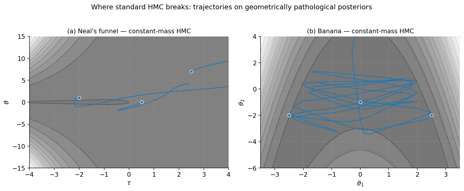
It stops working the moment local curvature varies across the support. Three textbook examples expose the failure mode.

Neal’s funnel. Consider the hierarchical prior $\theta \mid \tau \sim \mathcal{N}(0, e^\tau)$ with $\tau \sim \mathcal{N}(0, 9)$. The marginal density on $(\tau, \theta)$ traces a horn-shaped support that’s narrow at one end — small $\tau$, where $\theta$ has variance near 1 — and broad at the other, where $\theta$ has variance $e^\tau$. A constant mass matrix forces a single step size. Too small, and HMC takes years to traverse the broad end; too large, and it shoots past the narrow neck on every iteration. The funnel is the canonical failure case in Bayesian hierarchical modeling — every practitioner has been bitten by it.

The banana. Take a bivariate Gaussian on $(\theta_1, \theta_2)$ and apply the warp $\theta_2 \mapsto \theta_2 + b(\theta_1^2 - a^2)$. The result is the banana distribution of Haario, Saksman, and Tamminen (2001) — a curved ridge whose orientation rotates as we move along it. The Fisher information here varies smoothly with position: where the ridge is steep, $G(\theta)$ has a strong off-diagonal; where it’s shallow, $G$ is nearly diagonal. Standard HMC with constant $M$ can’t reflect that local rotation, so trajectories either spiral away from the ridge (large $\epsilon$) or crawl along it (small $\epsilon$).

Ill-conditioned hierarchical likelihoods. Even outside designed pathologies, real models often have parameters that mix on wildly different scales — population-level versus group-level variance components, regression coefficients with very different prior scales. Each direction wants its own step size. A diagonal preconditioner helps a bit but only handles conditioning that’s constant across the support; anywhere the curvature changes with position, we’re back to the same trade-off.

The pattern that connects all three: the local Fisher information

$$G(\theta) \;=\; -\,\mathbb{E}_{y \mid \theta}\!\bigl[\nabla^2_\theta \log p(y \mid \theta)\bigr]$$

— the matrix of expected second derivatives of the log-likelihood, with the expectation taken over the data distribution at $\theta$ — is not constant, but standard HMC pretends it is.

step size ε:ε = 0.15L = 40 leapfrog steps, identity mass matrix

1.2 The geometric fix

The Girolami–Calderhead (2011) move is to stop pretending. We promote the mass matrix from a constant to a function of position: $M(\theta) = G(\theta)$, with $G$ the Fisher information at $\theta$. The Hamiltonian becomes

$$H(\theta, p) \;=\; U(\theta) \;+\; \tfrac{1}{2}\, p^\top G(\theta)^{-1} p \;+\; \tfrac{1}{2}\,\log\det G(\theta),$$

where $U(\theta) = -\log p(\theta \mid y)$ is the negative log-posterior (our potential energy), and the extra log-determinant comes from normalizing the momentum’s conditional distribution $p \mid \theta \sim \mathcal{N}(0, G(\theta))$ at each position. Read geometrically, this says: parameter space is a Riemannian manifold equipped with the Fisher metric, momentum lives in the cotangent bundle, and Hamiltonian flow now follows geodesics of the manifold rather than straight lines.

The pathology of the funnel and the banana evaporates in this picture. Where the original geometry was steep, $G(\theta)$ is large and the metric scales the local step accordingly; where the geometry was loose, $G(\theta)$ is small and the step opens up. The same nominal $\epsilon$ now produces locally-appropriate motion everywhere.

There’s a cost. The new Hamiltonian is not separable — $H(\theta, p)$ doesn’t split into a $U(\theta) + K(p)$ form, because the kinetic part $K$ depends on $\theta$ through $G(\theta)$. The standard explicit leapfrog loses its symplecticity in that case, so we have to upgrade to an implicit integrator: each leapfrog step solves a fixed-point equation for the new momentum, and another for the new position. Each step also requires factorizing $G(\theta)$ — typically by Cholesky, since we need both $G^{-1}$ and $\det G$.

For the targets RMHMC is designed for, the cost is worth it. For an isotropic Gaussian on a well-conditioned likelihood, it isn’t. §8 makes this trade quantitative.

1.3 What you’ll need from elsewhere

This is an advanced topic and we lean heavily on the foundation.

From formalStatistics: bayesian-computation-and-mcmc , we assume comfortable familiarity with §26.9–10 on standard HMC: the canonical joint $\pi(\theta, p) \propto e^{-H(\theta, p)}$, Hamilton’s equations, the leapfrog integrator’s symplecticity and reversibility, the Metropolis correction, and the No-U-Turn heuristic for trajectory length. §2 here is a notation refresher, not a re-derivation. The §26.10 Remark 29 forward-pointer to Riemannian-manifold methods is discharged by the present topic.

From Information Geometry, we use the Fisher information metric and Čencov’s uniqueness theorem. The Fisher metric will be the mass matrix; we want the reader to recognize that this is not an arbitrary choice but the canonical Riemannian structure on the manifold of probability distributions — the unique (up to scale) metric invariant under sufficient statistics.

From Riemannian Geometry and Geodesics and Curvature, we use the metric tensor, the geodesic equation, Christoffel symbols, and parallel transport. RMHMC’s Hamiltonian flow is geodesic flow on the manifold of distributions, perturbed by the gradient of the potential.

From formalcalculus, we use the formalCalculus: jacobian for the volume-preservation theorem in §6 and the formalCalculus: inverse-implicit for the well-posedness of the implicit leapfrog in §5.

From the Stochastic-Gradient MCMC topic shipped earlier in T5, §10 introduced the position-dependent Riemannian metric in the SDE setting — RSGLD. We treat that as the SDE companion; the present topic does the Hamiltonian-flow side.

1.4 The Girolami–Calderhead 2011 program

The defining paper of Riemannian-manifold MCMC is Mark Girolami and Ben Calderhead’s “Riemann manifold Langevin and Hamiltonian Monte Carlo methods” (Journal of the Royal Statistical Society, Series B, vol. 73, 2011), with discussion. The paper does several things at once. It introduces the Riemann-manifold Langevin algorithm (RMLA) and Riemann-manifold HMC (RMHMC) as a pair, with the Fisher information as the canonical metric tensor for both. It works through the differential geometry needed for non-statisticians, derives the generalized leapfrog integrator, and provides three substantial empirical demonstrations: the banana distribution, a stochastic-volatility model, and a log-Gaussian Cox process for spatial statistics. The discussion section runs more than thirty pages and includes contributions from many of the leading figures in computational statistics.

The contribution that survives most cleanly into modern practice is the framework, not the specific integrator: the idea that a posterior’s local geometry can and should be exploited by gradient-based MCMC, and that the Fisher information is the natural carrier of that geometry. Variants and extensions have followed — SoftAbs metrics (Betancourt 2013) when the Fisher matrix is ill-defined or non-positive-definite, Hessian-based metrics for non-conjugate models, magnetic HMC, and the integration of RMHMC ideas into NUTS-style adaptive trajectory tuning. §12 surveys these.

1.5 Roadmap

The plan from here. §2 is a notation refresher for HMC — anyone who has read formalstatistics §26 can skim it. §3 rebuilds the Riemannian-geometry vocabulary we’ll need, anchored in the Fisher metric. §4 writes down the Riemannian Hamiltonian and Hamilton’s equations on the manifold; this is where the new log-determinant term gets interpreted. §5 is the core integrator construction: why the explicit leapfrog fails, what the implicit splitting looks like, and how to actually solve the fixed-point system in code. §6 collects the three load-bearing proofs — volume preservation, reversibility, detailed balance. §7 discusses tuning. §8 is the cost analysis. §§9–10 are worked examples: the banana, then a downsized log-Gaussian Cox process. §11 is the implementation patterns the project enforces — buffer hoisting, SPD-stable solves, multi-chain diagnostics. §12 zooms out to natural gradient, position-dependent SDEs, and the active research frontier.

The notebook tracks the brief section-for-section. Every section that carries new math has both expository markdown and validating code; §§9–10 are entirely empirical.

---

§2. HMC at a glance

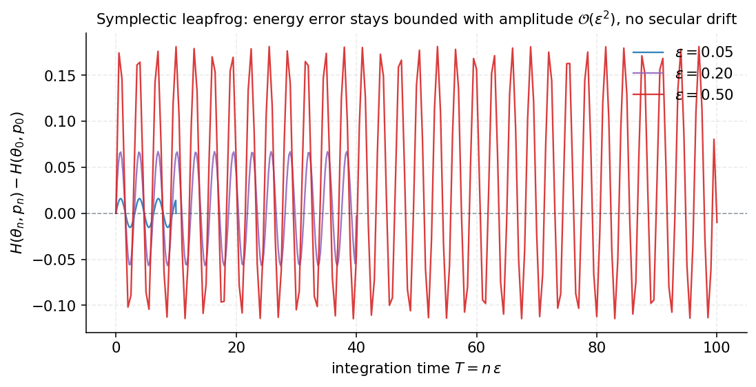
This section establishes the notation and the three properties of the standard leapfrog integrator — symplecticity, reversibility, energy conservation up to bounded oscillation — that the rest of the topic rebuilds for the new integrator. We assume the reader has worked through standard HMC in formalStatistics: bayesian-computation-and-mcmc §26.9–10 or Neal (2011); the treatment here is consciously compressed. If anything below feels like new material rather than recall, that’s a signal to read the prereqs before continuing.

2.1 The Hamiltonian and the canonical joint

Let $\pi(\theta) \propto e^{-U(\theta)}$ denote our target distribution on $\mathbb{R}^d$, where $U(\theta) = -\log \pi(\theta)$ (up to additive constants) is the potential energy — the negative log-target. HMC augments parameter space with an auxiliary momentum variable $p \in \mathbb{R}^d$ and constructs a joint distribution

$$\pi(\theta, p) \;\propto\; \exp\!\bigl(-H(\theta, p)\bigr), \qquad H(\theta, p) \;=\; U(\theta) \;+\; \tfrac{1}{2}\, p^\top M^{-1} p,$$

where $M \in \mathbb{R}^{d \times d}$ is a fixed, symmetric, positive-definite mass matrix and the second term is the kinetic energy $K(p) = \tfrac{1}{2} p^\top M^{-1} p$. Because $K$ depends only on $p$ (not on $\theta$), the joint factorizes: $\pi(\theta, p) = \pi(\theta) \cdot \mathcal{N}(p; 0, M)$. Marginalizing over $p$ recovers the target, so sampling $(\theta, p) \sim \pi$ and discarding $p$ samples $\theta \sim \pi(\theta)$ — the augmentation is “free.”

The Hamiltonian generates a continuous-time flow $\phi_t$ on $(\theta, p)$ space via Hamilton’s equations,

$$\frac{d\theta}{dt} \;=\; \frac{\partial H}{\partial p} \;=\; M^{-1} p, \qquad \frac{dp}{dt} \;=\; -\frac{\partial H}{\partial \theta} \;=\; -\nabla U(\theta).$$

Three properties of $\phi_t$ matter for what follows. First, $\phi_t$ preserves $H$ — the value of the Hamiltonian is constant along any flow trajectory, so trajectories stay on level sets of $H$. Second, $\phi_t$ is symplectic — it preserves the differential 2-form $\omega = \sum_i d\theta_i \wedge dp_i$, which in particular implies $\phi_t$ is volume-preserving on $(\theta, p)$ space. Third, $\phi_t$ is reversible under momentum negation: if we define $\mathcal{N}: (\theta, p) \mapsto (\theta, -p)$, then $\mathcal{N} \circ \phi_t \circ \mathcal{N} = \phi_{-t}$. These three together imply $\phi_t$ preserves the canonical measure $\pi(\theta, p)$ exactly — if we could integrate Hamilton’s equations in closed form, HMC would need no Metropolis correction. We can’t, so we discretize.

2.2 The leapfrog integrator

The natural discretization is the leapfrog (or Störmer–Verlet) integrator. From $(\theta^n, p^n)$, a single leapfrog step of size $\epsilon$ produces $(\theta^{n+1}, p^{n+1})$ via

$$\begin{aligned} p^{n+\tfrac{1}{2}} &= p^n - \tfrac{\epsilon}{2}\, \nabla U(\theta^n), \\ \theta^{n+1} &= \theta^n + \epsilon\, M^{-1} p^{n+\tfrac{1}{2}}, \\ p^{n+1} &= p^{n+\tfrac{1}{2}} - \tfrac{\epsilon}{2}\, \nabla U(\theta^{n+1}). \end{aligned}$$

The integrator is explicit — each line is a closed-form update — because $\nabla U$ depends only on $\theta$ and $M^{-1}p$ depends only on $p$. This is the defining structural property that breaks in §5: the Riemannian Hamiltonian’s kinetic term $\tfrac{1}{2} p^\top G(\theta)^{-1} p$ depends on $\theta$, so the position update becomes $\theta^{n+1} = \theta^n + \epsilon G(\theta^?)^{-1} p^{n+\tfrac{1}{2}}$, and we have to decide which $\theta$ to evaluate $G$ at — which is where implicitness enters.

Why the leapfrog works. Each of the three sub-steps is a shear in $(\theta, p)$ space: the momentum half-steps move $p$ at fixed $\theta$, and the position step moves $\theta$ at fixed $p$. Shears preserve the symplectic 2-form trivially, and the composition of symplectic maps is symplectic, so the full leapfrog map $\Phi_\epsilon: (\theta^n, p^n) \mapsto (\theta^{n+1}, p^{n+1})$ is symplectic — and therefore volume-preserving. The same symmetry of the three sub-steps about the central position update gives reversibility: $\Phi_\epsilon \circ \mathcal{N} \circ \Phi_\epsilon = \mathcal{N}$.

What the leapfrog does not preserve is $H$ exactly. It has $O(\epsilon^3)$ local error and $O(\epsilon^2)$ global error over a fixed integration time $T = L\epsilon$. But because the integrator is symplectic, the energy error oscillates around zero with bounded amplitude rather than drifting secularly — a result from backward error analysis (Hairer, Lubich, and Wanner 2006, ch. IX) that makes long-trajectory simulation feasible at moderate $\epsilon$. The Metropolis correction at the end of each trajectory restores exactness despite the residual integrator error, with acceptance probability $\alpha = \min\bigl(1, \exp(H(\theta^n, p^n) - H(\theta^{n+L}, p^{n+L}))\bigr)$.

2.3 Where the constant mass matrix becomes a ceiling

The mass matrix $M$ acts as a metric on momentum space. Reading $K(p) = \tfrac{1}{2} p^\top M^{-1} p$ geometrically: large $M$ in a direction means small kinetic energy contribution from large momentum in that direction, so trajectories cover ground faster there. The optimal choice for a Gaussian target $\mathcal{N}(\mu, \Sigma)$ is $M = \Sigma^{-1}$, which makes the level sets of $H$ spherical and decorrelates the leapfrog dynamics. Hoffman and Gelman’s NUTS (2014) and Stan’s adaptive HMC both estimate $M$ during warmup, typically as a diagonal or full-rank empirical-covariance preconditioner.

The estimate is global. It captures the average curvature of the target over the warmup chain. When the target’s actual local curvature varies smoothly with position — when the Fisher information matrix $G(\theta) = -\mathbb{E}_{y \mid \theta}[\nabla^2_\theta \log p(y \mid \theta)]$ depends on $\theta$ — no single constant $M$ can match all of it. Pick $M$ to suit the loose part of the support and the tight part rejects every proposal; pick $M$ to suit the tight part and the loose part mixes at glacial speed.

This is the gap. From §3 onward we promote $M$ to a function of $\theta$, recover the three properties of the leapfrog by other means (implicit splitting), and pay the per-step Cholesky cost in exchange for a step size that’s locally appropriate everywhere.

---

§3. Riemannian geometry of probability

The pieces this section assembles: the Fisher information matrix recast as a Riemannian metric, the cotangent picture of momentum that makes the RMHMC kinetic energy $\tfrac{1}{2} p^\top G(\theta)^{-1} p$ the natural choice rather than an arbitrary one, the geodesic equation in coordinate form, and Čencov’s uniqueness theorem. All of this material is developed at full length in Information Geometry and Riemannian Geometry; the present treatment stays terse and consciously selects what §§4–6 will need.

3.1 The Fisher information as a Riemannian metric

Let $\{p(y; \theta) : \theta \in \Theta \subseteq \mathbb{R}^d\}$ be a parametric family of probability densities on a sample space $\mathcal{Y}$, smooth in $\theta$. The score function is the gradient of the log-density,

$$s(y; \theta) \;=\; \nabla_\theta \log p(y; \theta) \;\in\; \mathbb{R}^d,$$

and under standard regularity (smooth interchange of $\nabla$ and $\int$), it has mean zero:

$$\mathbb{E}_{y \mid \theta}\bigl[s(y; \theta)\bigr] \;=\; \int p(y; \theta) \,\nabla_\theta \log p(y; \theta) \,dy \;=\; \nabla_\theta \!\int p(y; \theta)\, dy \;=\; \nabla_\theta(1) \;=\; 0.$$

The Fisher information matrix is the covariance of the score,

$$G(\theta) \;=\; \mathbb{E}_{y \mid \theta}\bigl[s(y; \theta)\, s(y; \theta)^\top\bigr] \;\in\; \mathbb{R}^{d \times d}.$$

A second differentiation gives the equivalent negative-expected-Hessian form. Starting from $\mathbb{E}_{y \mid \theta}[s(y; \theta)] = 0$ and differentiating in $\theta$ again,

$$0 \;=\; \nabla_\theta \!\int p(y; \theta)\, s(y; \theta)^\top \,dy \;=\; \int \bigl[\nabla_\theta p(y; \theta)\bigr] s(y; \theta)^\top \,dy \;+\; \int p(y; \theta)\, \nabla_\theta s(y; \theta)^\top \,dy.$$

The first integrand is $p \cdot s \cdot s^\top$ (using $\nabla_\theta p = p \cdot s$) and the second is $p \cdot \nabla^2_\theta \log p$, so

$$\mathbb{E}_{y \mid \theta}\bigl[s\, s^\top\bigr] \;+\; \mathbb{E}_{y \mid \theta}\bigl[\nabla^2_\theta \log p\bigr] \;=\; 0, \qquad\text{i.e.,}\qquad G(\theta) \;=\; -\,\mathbb{E}_{y \mid \theta}\bigl[\nabla^2_\theta \log p(y; \theta)\bigr].$$

A third equivalent form recovers the connection to information divergences: $G(\theta)$ is the Hessian of the KL divergence at the diagonal,

$$G_{ij}(\theta) \;=\; \frac{\partial^2}{\partial \theta'_i\, \partial \theta'_j}\, \mathrm{KL}\bigl(p(\cdot; \theta) \,\|\, p(\cdot; \theta')\bigr)\bigg|_{\theta' = \theta}.$$

This last identity — derived in the Information Geometry topic — is why $G(\theta)$ deserves the name “metric”: it measures, infinitesimally, the squared distance between $p(\cdot; \theta)$ and a nearby distribution. The pair $(\Theta, G)$ is a Riemannian manifold, and we’ll use $g_{ij}(\theta) = G_{ij}(\theta)$ when emphasizing the metric viewpoint and $G(\theta)$ when emphasizing the matrix viewpoint.

3.2 Cotangent vectors and index-raising

Stand at a point $\theta \in \Theta$. The tangent space $T_\theta \Theta \cong \mathbb{R}^d$ is the vector space of velocities — directions a parameter trajectory can move. The cotangent space $T_\theta^* \Theta \cong \mathbb{R}^d$ is its dual: the space of linear functionals on $T_\theta \Theta$. Concretely, a tangent vector $v \in T_\theta \Theta$ has components $v^i$ and a cotangent vector $p \in T_\theta^* \Theta$ has components $p_i$ — the index position records which kind of object you’re holding.

The metric gives a canonical isomorphism between the two spaces. Each tangent vector $v$ defines a cotangent vector $v^\flat$ via $v^\flat(w) = g_\theta(v, w)$ for any $w \in T_\theta \Theta$. In coordinates this is index lowering: $v_i = g_{ij}(\theta)\, v^j$, summing over the repeated index. The inverse map, index raising, sends a cotangent vector $p$ to the tangent vector $p^\sharp$ with components $p^i = g^{ij}(\theta)\, p_j$, where $g^{ij}(\theta)$ is the matrix inverse of $g_{ij}(\theta)$ — equivalently, $G(\theta)^{-1}$.

Why this matters for RMHMC. Position $\theta$ lives on the manifold and its velocity $\dot\theta$ is naturally a tangent vector. Momentum $p$, the conjugate variable, is naturally a cotangent vector — it pairs with velocity via the Lagrangian formulation, $p_i = \partial L / \partial \dot\theta^i$, which lands in the dual space. The kinetic energy is the squared norm of $p$ measured in the inverse metric on the cotangent space:

$$K(\theta, p) \;=\; \tfrac{1}{2}\, \langle p, p\rangle_{g^*} \;=\; \tfrac{1}{2}\, g^{ij}(\theta)\, p_i\, p_j \;=\; \tfrac{1}{2}\, p^\top G(\theta)^{-1} p.$$

This is exactly the kinetic term in the Girolami–Calderhead Hamiltonian. The $G(\theta)^{-1}$ is doing index-raising — converting the cotangent momentum into the tangent velocity $\dot\theta = G(\theta)^{-1} p$, which is what Hamilton’s first equation will say in §4. Read this way, the RMHMC kinetic energy isn’t a clever choice; it’s the unique kinetic energy compatible with treating momentum as a cotangent vector and the metric as Fisher.

3.3 Geodesics, Christoffel symbols, and the geodesic equation

On a flat manifold, a free particle moves in a straight line. On a curved one, “straight” gets replaced by geodesic — the curve that locally minimizes arc length, or equivalently, the curve whose tangent vector parallel-transports along itself. In coordinates, a curve $\theta(t)$ is a geodesic of $(\Theta, g)$ if

$$\ddot\theta^{\,k} \;+\; \Gamma^k_{ij}(\theta)\, \dot\theta^{\,i}\, \dot\theta^{\,j} \;=\; 0, \qquad k = 1, \dots, d,$$

with Einstein summation over $i, j$. The Christoffel symbols $\Gamma^k_{ij}$ are determined by the metric:

$$\Gamma^k_{ij}(\theta) \;=\; \tfrac{1}{2}\, g^{kl}(\theta)\, \bigl(\partial_i\, g_{jl}(\theta) \;+\; \partial_j\, g_{il}(\theta) \;-\; \partial_l\, g_{ij}(\theta)\bigr).$$

These are not tensor components — they transform inhomogeneously under coordinate changes — but the geodesic equation as a whole is coordinate-invariant. On a flat manifold ($g_{ij}$ constant), all $\Gamma^k_{ij} \equiv 0$ and the equation collapses to $\ddot\theta = 0$, recovering Newton’s first law.

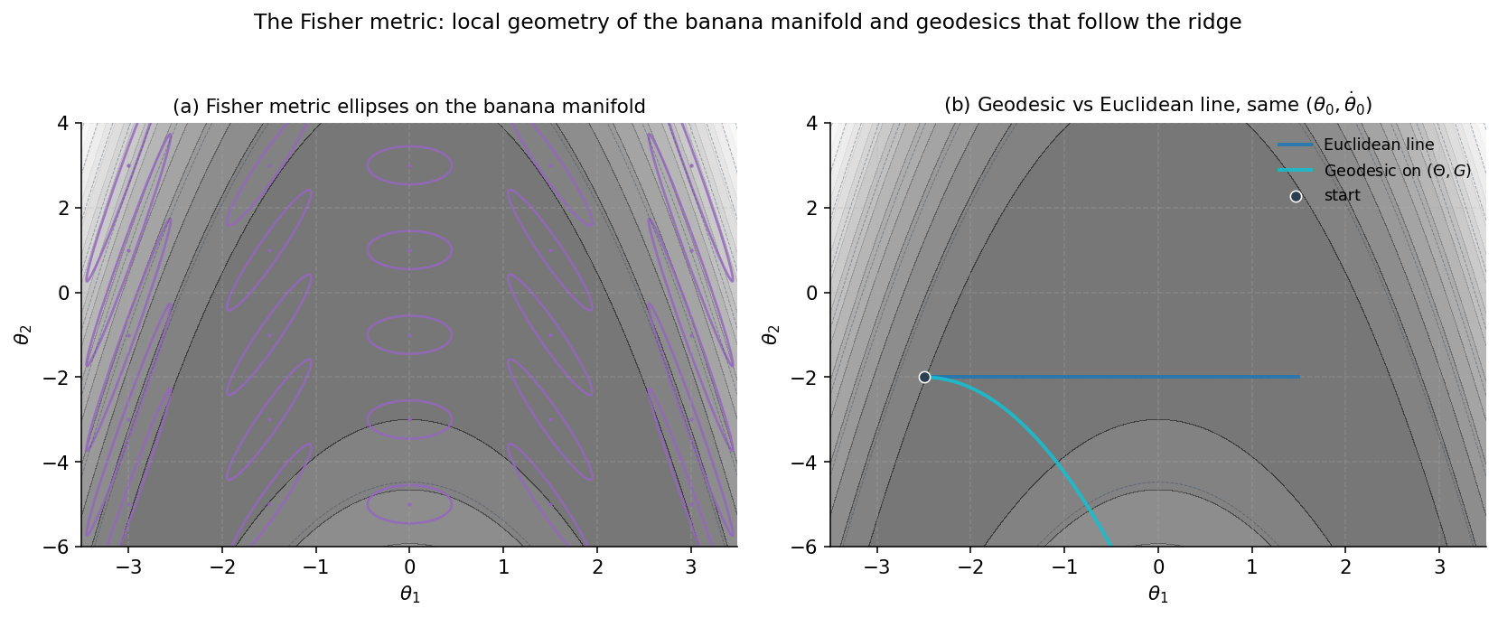
What this means for RMHMC. Hamilton’s equations on $(\Theta, g)$, derived in §4, contain Christoffel-symbol-like terms in the momentum update — the price of position-dependent kinetic energy. When the potential $U(\theta)$ is zero, Hamilton’s equations on the manifold reduce exactly to the geodesic equation: the leapfrog integrator becomes a geodesic integrator, and the trajectory follows the geometry of $(\Theta, g)$ with no external force. When $U \ne 0$, we get geodesic flow perturbed by $-\nabla U(\theta)$. The pathological posteriors of §1 are pathological precisely because their flat trajectories don’t track the manifold’s geometry; their geodesic trajectories do.

For the banana model of §9, the only nonzero Christoffel symbol turns out to be $\Gamma^2_{11} = 2b$ — and that single component is exactly what’s needed to bend the geodesic into the ridge’s curvature. The viz below demonstrates this with a corrected closed-form Christoffel computation; the static fallback PNG uses a slightly off implementation from the notebook and may show the geodesic curving the wrong direction, so trust the live viz for the geometric story.

banana curvature b:b = 1.00start:(-2, -3) — on ridge(-2.5, -2) — above ridge(0, -1) — near centerridge-tangent initial velocity

3.4 Čencov’s uniqueness

Why the Fisher metric and not some other position-dependent metric? Čencov’s theorem (Čencov 1972, refined by Campbell 1986; see Information Geometry for full proof) answers this.

Translated: take any parametric family $\{p(y; \theta)\}$ and any sufficient statistic $T(y)$ for it; the induced family $\{p(T(y); \theta)\}$ has its own statistical manifold, and the Fisher metric on the original manifold pushes forward to the Fisher metric on the new one. No other Riemannian metric on statistical manifolds has this invariance property.

For RMHMC, this is the foundational sanity check: the choice of position-dependent metric is not arbitrary tuning. The Fisher information is the unique canonical Riemannian structure on a manifold of distributions. Variants — SoftAbs, observed Hessian, Hessian-based metrics — sacrifice this invariance to gain computational tractability or PSD-ness. They are useful approximations; Fisher is the reference point against which they are judged.

---

§4. The Riemannian Hamiltonian

Standard HMC’s mass matrix was a single constant. The promotion to a position-dependent metric — $M(\theta) = G(\theta)$ with $G$ the Fisher information — changes three things at once: the momentum distribution, the kinetic energy, and the Hamiltonian itself. The third change is the subtle one: an extra log-determinant term appears in $H$, and it has to be there for the marginalization to recover the target. This section assembles all of it.

4.1 The position-dependent mass matrix

In standard HMC, the mass matrix $M \in \mathbb{R}^{d \times d}$ is a fixed SPD matrix — typically the identity, or a covariance estimate from warmup. Read through the §3.2 lens, $M$ functions as a metric on momentum space: it tells us how to convert a cotangent vector (momentum) into a tangent vector (velocity) via $\dot\theta = M^{-1} p$, and how to assign a squared norm to momentum via $K(p) = \tfrac{1}{2} p^\top M^{-1} p$.

RMHMC’s move is to let this metric depend on position. We set $M(\theta) = G(\theta)$, where $G$ is the Fisher information matrix at $\theta$ (canonically; see §3 for the why-Fisher argument). The momentum’s conditional distribution becomes $p \mid \theta \sim \mathcal{N}(0, G(\theta))$ — a Gaussian whose covariance changes with where we are on the manifold. In coordinates where the manifold has high local curvature (large eigenvalues of $G$), momentum is sampled with large variance, so trajectories explore vigorously in that region; where curvature is low, momentum is small and trajectories crawl. This is the inverse of what standard HMC does with a constant $M$ — there, momentum scale is fixed, and pathological geometry punishes the trajectory.

Two consequences are immediate and matter for everything that follows. The kinetic energy gains $\theta$-dependence: $K(\theta, p) = \tfrac{1}{2} p^\top G(\theta)^{-1} p$. And because the momentum density $\mathcal{N}(0, G(\theta))$ has a $\theta$-dependent normalizing constant, the joint density we’re sampling from will need an explicit log-determinant correction to remain consistent with the target. We work that out next.

4.2 The augmented joint density

The target is $\pi(\theta) \propto e^{-U(\theta)}$ with $U(\theta) = -\log \pi(\theta)$. Augment with momentum $p \mid \theta \sim \mathcal{N}(0, G(\theta))$. The joint is the product of the marginal and the conditional:

$$\pi(\theta, p) \;=\; \pi(\theta) \cdot \frac{1}{\sqrt{(2\pi)^d\, \det G(\theta)}} \exp\!\Bigl(-\tfrac{1}{2}\, p^\top G(\theta)^{-1} p\Bigr).$$

Take the negative log and collect terms up to additive constants in $(\theta, p)$:

$$H(\theta, p) \;=\; -\log \pi(\theta, p) \;=\; U(\theta) \;+\; \tfrac{1}{2}\, p^\top G(\theta)^{-1} p \;+\; \tfrac{1}{2}\, \log\det G(\theta).$$

This is the Girolami–Calderhead Hamiltonian. The three terms are the potential energy $U(\theta)$, the position-dependent kinetic energy $K(\theta, p) = \tfrac{1}{2} p^\top G(\theta)^{-1} p$, and a new volume term $V(\theta) = \tfrac{1}{2} \log\det G(\theta)$ that wasn’t there in flat-space HMC.

The volume term is exactly what’s needed for marginal correctness. Marginalize $p$ from the joint $\pi(\theta, p) \propto e^{-H(\theta, p)}$:

$$\int e^{-H(\theta, p)}\, dp \;=\; e^{-U(\theta)} \cdot e^{-\tfrac{1}{2}\log\det G(\theta)} \cdot \int e^{-\tfrac{1}{2} p^\top G(\theta)^{-1} p}\, dp.$$

The remaining Gaussian integral evaluates to $(2\pi)^{d/2} \sqrt{\det G(\theta)}$, so the right-hand side simplifies to $(2\pi)^{d/2}\, e^{-U(\theta)} \propto \pi(\theta)$. The $\sqrt{\det G(\theta)}$ from the Gaussian normalizer exactly cancels the $e^{-\tfrac{1}{2}\log\det G}$ from the volume term, leaving the target. Drop the volume term and the marginal would be wrong — it would be proportional to $\pi(\theta) / \sqrt{\det G(\theta)}$, which is not what we want to sample.

This is also why the volume term cannot be absorbed into $U(\theta)$ as a redefinition of the potential. It must appear in $H$ precisely as written, because the same factor of $\sqrt{\det G(\theta)}$ also appears in the momentum normalizer that the sampler implicitly uses every time it draws a momentum, and the two have to cancel.

4.3 The three terms

Let’s interpret each piece of $H = U + K + V$.

The potential energy $U(\theta) = -\log \pi(\theta)$ is unchanged from flat-space HMC. It tells the dynamics where the target prefers to be: gradients of $U$ pull trajectories toward high-density regions of $\pi$.

The kinetic energy $K(\theta, p) = \tfrac{1}{2} p^\top G(\theta)^{-1} p$ is now position-dependent. Read geometrically, $K$ is the squared norm of the cotangent momentum $p$ measured in the inverse metric — exactly the construction of §3.2. The position-dependence makes $K$ non-separable from $\theta$: the kinetic and potential coordinates are entangled by the metric. This is the property that breaks the explicit leapfrog in §5.

The volume term $V(\theta) = \tfrac{1}{2}\log\det G(\theta)$ is the new piece. It’s a purely geometric potential — it depends only on the manifold, not on the target. We can think of it as a “geometric correction” that prevents the dynamics from preferring high-determinant regions of the manifold over low-determinant ones. Without $V$, regions where $G(\theta)$ has large eigenvalues would oversample momentum and skew the joint.

A useful regrouping is $\tilde{U}(\theta) = U(\theta) + V(\theta)$ — the augmented potential — so that $H(\theta, p) = \tilde{U}(\theta) + K(\theta, p)$. Hamilton’s equations on $(\theta, p)$ space then look more familiar: the gradient force is $-\nabla \tilde{U}$, splitting into a target-driven part and a geometry-driven part.

4.4 Hamilton’s equations on the manifold

Hamilton’s equations are $\dot\theta^i = \partial H/\partial p_i$ and $\dot p_i = -\partial H/\partial \theta^i$. With our three-term $H$, the position update is immediate:

$$\dot\theta \;=\; \frac{\partial H}{\partial p} \;=\; G(\theta)^{-1}\, p.$$

This is just the cotangent-to-tangent index-raising of §3.2 — the position evolves with velocity equal to the momentum’s tangent representative.

The momentum update requires differentiating each term of $H$ with respect to $\theta_k$. The potential gives $\partial_k U$. The kinetic term gives $\tfrac{1}{2} p^\top \partial_k(G^{-1}) p$, and using the matrix identity $\partial_k G^{-1} = -G^{-1}(\partial_k G)\, G^{-1}$, this becomes $-\tfrac{1}{2} p^\top G^{-1} (\partial_k G)\, G^{-1} p$. The volume term gives $\tfrac{1}{2}\, \partial_k \log\det G = \tfrac{1}{2}\, \mathrm{tr}\bigl(G^{-1}\, \partial_k G\bigr)$ via the Jacobi formula. Collecting,

$$\dot p_k \;=\; -\,\partial_k U(\theta) \;+\; \tfrac{1}{2}\, p^\top G(\theta)^{-1} (\partial_k G(\theta))\, G(\theta)^{-1} p \;-\; \tfrac{1}{2}\, \mathrm{tr}\bigl(G(\theta)^{-1}\, \partial_k G(\theta)\bigr).$$

Three forces are visible. The first is the gradient of the potential — the same as standard HMC. The second is a Coriolis-like force: it is quadratic in momentum, depends on the derivative of the metric, and vanishes when the metric is constant. The third is the gradient of the volume potential, $-\partial_k V$.

The Coriolis term is what connects the dynamics to geodesic flow on the manifold. Substituting $\dot\theta = G^{-1} p$ into the quadratic-in-$p$ term, it becomes $\tfrac{1}{2}\, \dot\theta^\top (\partial_k G(\theta))\, \dot\theta$, which after some index gymnastics combines with $\partial_k$ of the kinetic energy to produce exactly the Christoffel-symbol contraction of §3.3. Concretely: when $U \equiv 0$ and $V \equiv 0$, the Hamiltonian flow reduces to

$$\ddot\theta^{\,k} \;+\; \Gamma^k_{ij}(\theta)\, \dot\theta^{\,i}\, \dot\theta^{\,j} \;=\; 0,$$

the geodesic equation. With $U$ and $V$ present, we get geodesic flow perturbed by $-\nabla \tilde{U}$.

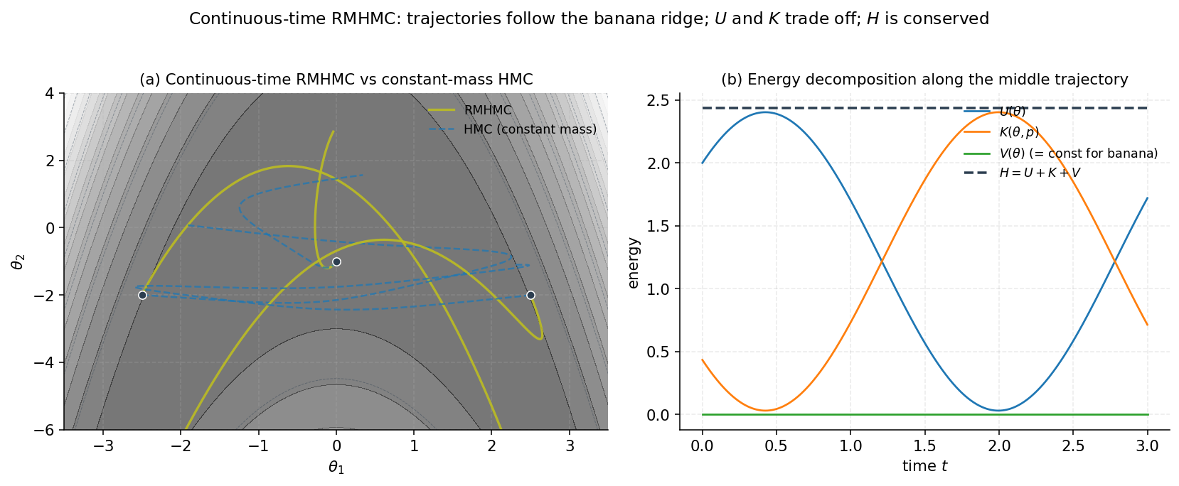
This is the picture to hold onto: continuous-time RMHMC is geodesic flow on the manifold of distributions, perturbed by the gradient of the augmented potential. In continuous time, the flow conserves $H$ exactly and preserves $\pi(\theta, p) \propto e^{-H}$ exactly. The problem §5 has to solve is how to discretize this flow in a way that still preserves the canonical measure — at least to the accuracy needed for a Metropolis correction to make up the residual error.

integration time T:T = 3.0show HMC comparisonreset startsClick panel (a) to add a start (rolls oldest off).

---

§5. The Generalized Leapfrog Integrator

Continuous-time RMHMC preserves the canonical measure exactly. The discrete version cannot — we have to integrate Hamilton’s equations approximately, and any approximation introduces error. The question is whether we can choose the discrete integrator so that the structural properties — symplecticity, reversibility, volume preservation — survive the discretization, leaving only a bounded energy error that the Metropolis correction can mop up. The standard leapfrog of §2 does this for separable Hamiltonians. The Riemannian Hamiltonian is non-separable, and the standard leapfrog fails. The fix is to make the integrator implicit.

5.1 Non-separability and what it breaks

Recall the standard leapfrog of §2. It comes from the splitting $H(\theta, p) = U(\theta) + K(p)$ — potential energy depends only on $\theta$, kinetic energy depends only on $p$. The integrator alternates shears: a half-step of $p$ at fixed $\theta$ (using $\partial U/\partial \theta$), a full step of $\theta$ at fixed $p$ (using $\partial K/\partial p$), and another half-step of $p$. Each substep is a symplectic shear because it updates only one of the two variables, and the composition of symplectic maps is symplectic. The proof in §2 was almost trivial.

For the Riemannian Hamiltonian $H(\theta, p) = U(\theta) + V(\theta) + \tfrac{1}{2} p^\top G(\theta)^{-1} p$, the kinetic energy $K(\theta, p)$ depends on both variables — the metric $G$ depends on position. The standard shear-based splitting no longer applies. If we try to write the same three-step structure naively — “half-step in $p$ using $\nabla U$, full step in $\theta$ using $G^{-1} p$, another half-step in $p$” — three things go wrong. First, the half-step in $p$ would miss the contribution $\partial K/\partial \theta$ to $\dot p$, so it’s not the right gradient. Second, even if we included $\partial K/\partial \theta$, the substep is no longer a shear: it updates $p$ at fixed $\theta$ but with a gradient that depends on the same $p$ we’re updating. Third, the resulting map is not symplectic — energy drifts secularly with $n$, and after a few hundred leapfrog steps the chain is sampling from the wrong distribution.

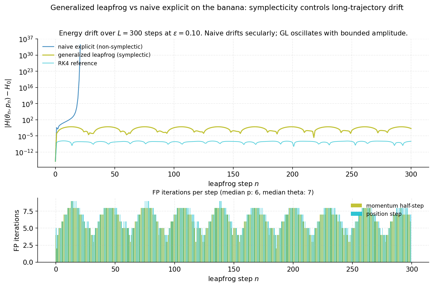
The pathology is reproducible and visible. The naive explicit Riemannian leapfrog applied to the banana shows $|H(\theta_n, p_n) - H_0|$ growing roughly linearly with $n$, never returning to baseline — the hallmark of a non-symplectic integrator. The generalized leapfrog, by contrast, keeps the energy error bounded just as the standard leapfrog did in §2.

5.2 The Leimkuhler–Reich splitting

The fix, due to Leimkuhler and Reich (2004, ch. 4), is to keep the three-step symmetric structure but allow each step to be defined implicitly. The integrator is sometimes called the Störmer–Verlet for general Hamiltonians or the generalized leapfrog; we’ll use the latter name throughout. For a step of size $\epsilon$ from $(\theta^n, p^n)$ to $(\theta^{n+1}, p^{n+1})$,

$$\begin{aligned} p^{n+\tfrac{1}{2}} &= p^n - \tfrac{\epsilon}{2}\, \nabla_\theta H\!\bigl(\theta^n,\, p^{n+\tfrac{1}{2}}\bigr), \\ \theta^{n+1} &= \theta^n + \tfrac{\epsilon}{2}\, \bigl[\nabla_p H\!\bigl(\theta^n,\, p^{n+\tfrac{1}{2}}\bigr) \,+\, \nabla_p H\!\bigl(\theta^{n+1},\, p^{n+\tfrac{1}{2}}\bigr)\bigr], \\ p^{n+1} &= p^{n+\tfrac{1}{2}} - \tfrac{\epsilon}{2}\, \nabla_\theta H\!\bigl(\theta^{n+1},\, p^{n+\tfrac{1}{2}}\bigr). \end{aligned}$$

Two of the three lines are implicit. The first defines $p^{n+1/2}$ via an equation whose right-hand side depends on $p^{n+1/2}$ — the gradient $\nabla_\theta H$ contains the kinetic-energy gradient $\nabla_\theta K(\theta, p)$, which is quadratic in the momentum we’re trying to compute. The second defines $\theta^{n+1}$ via an equation whose right-hand side contains $\nabla_p H(\theta^{n+1}, p^{n+1/2}) = G(\theta^{n+1})^{-1} p^{n+1/2}$ — the new position appears inside the metric. Only the third step is explicit, because by then both $\theta^{n+1}$ and $p^{n+1/2}$ are known.

The symmetric structure is what makes this work. The map $(\theta^n, p^n) \mapsto (\theta^{n+1}, p^{n+1})$ defined by the three lines above is the composition of two pieces: a half-Hamiltonian-flow under a frozen-metric Hamiltonian and a half-Hamiltonian-flow under the full position-dependent one. Each is a true Hamiltonian flow, hence symplectic; the composition is symplectic. We prove this carefully in §6.

5.3 The two implicit momentum half-steps

Specialize to the Riemannian Hamiltonian. With $\nabla_p H(\theta, p) = G(\theta)^{-1} p$ and $\nabla_\theta H(\theta, p) = \nabla U(\theta) + \nabla V(\theta) + \nabla_\theta K(\theta, p)$, where the kinetic-energy gradient has components

$$\bigl[\nabla_\theta K(\theta, p)\bigr]_k \;=\; -\tfrac{1}{2}\, p^\top G(\theta)^{-1} \bigl(\partial_k G(\theta)\bigr)\, G(\theta)^{-1} p,$$

the first leapfrog line becomes

$$p^{n+\tfrac{1}{2}} \;=\; p^n \;-\; \tfrac{\epsilon}{2}\, \nabla U(\theta^n) \;-\; \tfrac{\epsilon}{2}\, \nabla V(\theta^n) \;-\; \tfrac{\epsilon}{2}\, \nabla_\theta K\!\bigl(\theta^n,\, p^{n+\tfrac{1}{2}}\bigr).$$

The first three terms on the right are constants once $\theta^n$ is known. The fourth term is the implicit one: it’s quadratic in $p^{n+1/2}$ through the structure $\nabla_\theta K \propto p^\top \mathrm{Tensor}(\theta) p$. Write the equation as

$$p^{n+\tfrac{1}{2}} \;=\; b \;-\; \tfrac{\epsilon}{2}\, \nabla_\theta K\!\bigl(\theta^n,\, p^{n+\tfrac{1}{2}}\bigr), \qquad b \;:=\; p^n - \tfrac{\epsilon}{2}\,\bigl[\nabla U(\theta^n) + \nabla V(\theta^n)\bigr].$$

Solve by fixed-point iteration: starting from $p^{(0)} = b$, iterate

$$p^{(k+1)} \;=\; b \;-\; \tfrac{\epsilon}{2}\, \nabla_\theta K\!\bigl(\theta^n,\, p^{(k)}\bigr)$$

until $\|p^{(k+1)} - p^{(k)}\| < \mathrm{tol}$. The metric $G(\theta^n)$ doesn’t change across iterations, so a single Cholesky factorization of $G(\theta^n)$ — computed once before the iteration — provides $G(\theta^n)^{-1}$ for every evaluation of $\nabla_\theta K$. This is the main reason the per-step cost is dominated by one Cholesky per half-step rather than one per iteration.

The third leapfrog line is the same form but explicit: once we know $\theta^{n+1}$ and $p^{n+1/2}$, the right-hand side is just

$$p^{n+1} \;=\; p^{n+\tfrac{1}{2}} \;-\; \tfrac{\epsilon}{2}\,\bigl[\nabla U(\theta^{n+1}) + \nabla V(\theta^{n+1}) + \nabla_\theta K\!\bigl(\theta^{n+1},\, p^{n+\tfrac{1}{2}}\bigr)\bigr].$$

This requires the Cholesky of $G(\theta^{n+1})$, which we’ll have computed during step 2 and can reuse.

5.4 The implicit position update

The middle line is

$$\theta^{n+1} \;=\; \theta^n \;+\; \tfrac{\epsilon}{2}\,\bigl[G(\theta^n)^{-1} + G(\theta^{n+1})^{-1}\bigr] p^{n+\tfrac{1}{2}}.$$

The first metric inverse is known. The implicit part is the second term, $G(\theta^{n+1})^{-1} p^{n+1/2}$, which requires the metric at the unknown new position. Write the equation as

$$\theta^{n+1} \;=\; c \;+\; \tfrac{\epsilon}{2}\, G(\theta^{n+1})^{-1} p^{n+\tfrac{1}{2}}, \qquad c \;:=\; \theta^n + \tfrac{\epsilon}{2}\, G(\theta^n)^{-1} p^{n+\tfrac{1}{2}}.$$

Fixed-point iteration starts from $\theta^{(0)} = c$ and iterates

$$\theta^{(k+1)} \;=\; c \;+\; \tfrac{\epsilon}{2}\, G(\theta^{(k)})^{-1} p^{n+\tfrac{1}{2}}$$

until convergence. Each iteration computes a fresh Cholesky of $G(\theta^{(k)})$. This is where the per-step cost can balloon — if convergence takes 10 iterations, that’s 10 Choleskys for this single step. Typical $\epsilon$ regimes get away with 3–5 iterations; outside that regime, the integrator is signaling that $\epsilon$ is too large.

A semi-explicit simplification is available when the metric has structure. If $G(\theta)$ is block-diagonal in the parameter space and one block depends only on a parameter subgroup that this step’s $p^{n+1/2}$ projects onto trivially, the position update for that subgroup is closed-form. For the log-Gaussian Cox process in §10, the GMRF-prior block of $G$ is constant, and only the likelihood-Fisher block requires iteration.

5.5 Fixed-point iteration in practice

Three implementation concerns turn out to matter.

Existence and uniqueness. The implicit function theorem (see formalCalculus: inverse-implicit ) guarantees that for $\epsilon$ small enough, both implicit equations have unique solutions. The argument: at $\epsilon = 0$, both maps are the identity, and the Jacobian of the fixed-point equation at $\epsilon = 0$ is the identity matrix. The IFT extends this to a neighborhood of $\epsilon = 0$.

Tolerance and warm-starting. The standard tolerance is $\mathrm{tol} = 10^{-6}$ in the relative-change norm $\|\Delta\|/\|p^{(k)}\|$ for the momentum half-step and analogously for the position. This is far below the discretization error of the integrator itself, so the fixed-point precision is not the binding constraint on chain accuracy — the leapfrog step size is. Warm-start the iteration from the explicit (zeroth-order) update: $p^{(0)} = b$ for the momentum half-step, $\theta^{(0)} = c$ for the position step. With a tight $\epsilon$, this warm-start often produces convergence within one or two iterations.

Divergence diagnostics. If the iteration counter exceeds a cap (typical: 20 iterations) without convergence, treat the leapfrog step as divergent — abort the trajectory, reject the proposal (acceptance probability 0), and increment a divergence counter for that chain. NUTS practice treats divergences as a hard signal that warmup-time $\epsilon$ adaptation should reduce step size; RMHMC inherits the same heuristic. A chain that produces more than ~1% divergent transitions has $\epsilon$ too large for the local geometry it’s exploring.

step size ε:ε = 0.15steps L:L = 200divergence cap:

---

§6. Volume preservation, reversibility, and detailed balance

Continuous-time Hamiltonian flow preserves the canonical measure $\pi(\theta, p) \propto e^{-H(\theta, p)}$ exactly. A discrete integrator cannot — there is always some discretization error in $H$. The Metropolis correction handles that error by accepting or rejecting proposals based on the energy difference. But the Metropolis correction itself relies on three structural properties of the proposal map: it must be volume-preserving in $(\theta, p)$-space, reversible under momentum negation, and produce a kernel that satisfies detailed balance. Standard HMC’s explicit leapfrog has these properties by inspection. The generalized leapfrog is not made of shears, so we have to prove them by direct calculation. Each of the three is load-bearing: drop volume preservation and the Jacobian factor in the acceptance ratio fails to collapse to 1; drop reversibility and the forward and reverse moves are no longer paired correctly; drop detailed balance and the chain doesn’t target the right distribution.

Throughout this section let $\Phi_\epsilon: (\theta^n, p^n) \mapsto (\theta^{n+1}, p^{n+1})$ denote one step of the generalized leapfrog of §5.2, and decompose it as $\Phi_\epsilon = \Phi^C_{\epsilon/2} \circ \Phi^B_\epsilon \circ \Phi^A_{\epsilon/2}$ where the substeps are the three lines of the integrator. Let $\mathcal{N}: (\theta, p) \mapsto (\theta, -p)$ denote momentum negation.

6.1 Volume preservation

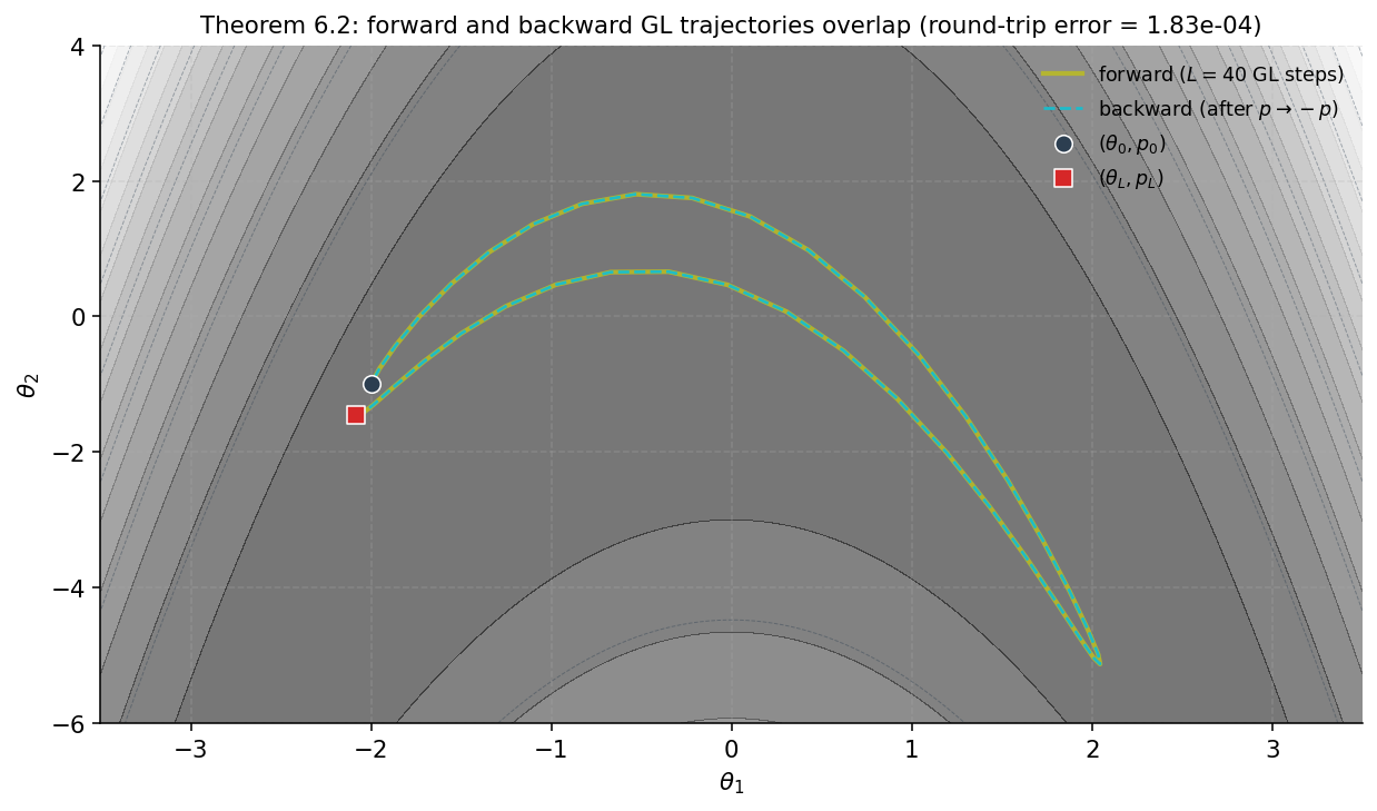
6.2 Reversibility

Composing $L$ leapfrog steps, the same argument by induction gives $\mathcal{N} \circ \Phi_\epsilon^L \circ \mathcal{N} = \Phi_\epsilon^{-L}$, so the trajectory of $L$ steps is reversible under momentum negation as a single unit.

step size ε:ε = 0.15steps L:L = 40round-trip error: 7.13e-6

6.3 Detailed balance

The RMHMC proposal map is $\Psi := \mathcal{N} \circ \Phi_\epsilon^L$ — run $L$ leapfrog steps, then negate momentum. By §6.2, $\Psi$ is an involution: $\Psi \circ \Psi = \mathrm{id}$. By §6.1, $|\det J_\Psi| = 1$ (the leapfrog has unit Jacobian; momentum negation has $|\det \mathcal{N}| = 1$). The Metropolis-corrected RMHMC kernel is

$$K\bigl((\theta, p) \to A\bigr) \;=\; \alpha(\theta, p)\, \mathbf{1}\!\bigl[\Psi(\theta, p) \in A\bigr] \;+\; \bigl(1 - \alpha(\theta, p)\bigr)\, \mathbf{1}\!\bigl[(\theta, p) \in A\bigr],$$

with acceptance probability $\alpha(\theta, p) = \min\bigl(1,\, e^{H(\theta, p) - H(\Psi(\theta, p))}\bigr)$.

6.4 The Jacobian-determinant collapse

The $\det G(\theta)$ factor that would normally appear in a Metropolis acceptance probability between distributions whose momentum-conditionals have different covariances does appear here — but it appears inside $H$, via the volume term $V(\theta) = \tfrac{1}{2} \log \det G(\theta)$, rather than as a separate Jacobian factor in front.

To see this, write out the energy difference along a transition:

$$H(\theta', p') - H(\theta, p) \;=\; \bigl[U(\theta') - U(\theta)\bigr] \;+\; \tfrac{1}{2}\log\frac{\det G(\theta')}{\det G(\theta)} \;+\; \bigl[K(\theta', p') - K(\theta, p)\bigr].$$

The middle term is exactly $\log\sqrt{\det G(\theta')/\det G(\theta)}$ — the log-ratio of the metric volumes at the two states. In exponentiating to get the acceptance probability,

$$\alpha \;=\; \min\!\Bigl(1,\, e^{H(\theta, p) - H(\theta', p')}\Bigr) \;=\; \min\!\biggl(1,\, e^{U(\theta) - U(\theta')} \cdot \sqrt{\tfrac{\det G(\theta)}{\det G(\theta')}} \cdot e^{K(\theta, p) - K(\theta', p)}\biggr),$$

the metric-volume factor multiplies the potential-energy and kinetic-energy ratios in exactly the way a change-of-measure factor would. The point is that we don’t compute it separately — packaging $V(\theta)$ into $H$ from §4.2 means a single energy difference automatically carries the metric-Jacobian correction. That is what the volume term does.

6.5 Putting it together

The RMHMC algorithm at each iteration:

1. Resample momentum from $p \sim \mathcal{N}(0, G(\theta))$ at the current $\theta$ — a Gibbs step in the augmented space.
2. Propose $\Psi(\theta, p)$ via $L$ generalized-leapfrog steps and momentum negation.
3. Accept or reject by the Metropolis rule of §6.3.

Step (i) is exact and leaves $\pi(\theta, p)$ invariant by construction. Step (ii)–(iii) leaves $\pi(\theta, p)$ invariant by detailed balance. Composing the two steps gives a kernel that’s $\pi(\theta, p)$-invariant. Marginalizing $p$ recovers $\pi(\theta)$.

The chain’s irreducibility, aperiodicity, and geometric-ergodicity properties are inherited from standard HMC under regularity conditions on the metric (Livingstone, Betancourt, Byrne, and Girolami 2019); §7 addresses what those conditions look like in practice.

---

§7. Step size, trajectory length, and ergodicity

Standard HMC has one main tuning knob — the leapfrog step size $\epsilon$ — plus a secondary one, the trajectory length $L$. RMHMC inherits both and adds a third: the implicit-solver tolerance and iteration cap. The interactions among the three are not what one would expect from naive intuition built on Euclidean HMC, and the practical guidance has to track that.

7.1 What controls the implicit-solver convergence

In standard HMC, $\epsilon$ controls accuracy: smaller $\epsilon$ means smaller per-step energy error and higher acceptance, at the price of more leapfrog steps to traverse the same trajectory time $T = L \epsilon$. There’s a single trade-off: $\epsilon$ vs $L$ at fixed $T$.

RMHMC adds a second constraint. The implicit fixed-point iteration of §5.5 has to converge, and its contraction rate depends on the local geometry. Look at the momentum half-step’s iteration map,

$$F_1(p^*) \;=\; b \;-\; \tfrac{\epsilon}{2}\, \nabla_\theta K(\theta^n, p^*),$$

where $\nabla_\theta K(\theta, p) = -\tfrac{1}{2} p^\top G(\theta)^{-1} (\partial_k G(\theta))\, G(\theta)^{-1} p$ in coordinates. The Jacobian of $F_1$ in $p^*$ is $-\tfrac{\epsilon}{2}\, \partial(\nabla_\theta K)/\partial p$, and its operator norm scales as $\epsilon \cdot \|G^{-1}(\theta^n)\| \cdot \|\partial G(\theta^n)\| \cdot \|G^{-1}(\theta^n)\| \cdot \|p\|$. The iteration is a contraction iff this norm is less than 1, which gives an effective $\epsilon$ constraint that depends on position:

$$\epsilon \;\lesssim\; \frac{1}{\|G^{-1}(\theta^n)\|^2 \cdot \|\nabla G(\theta^n)\| \cdot \|p\|}.$$

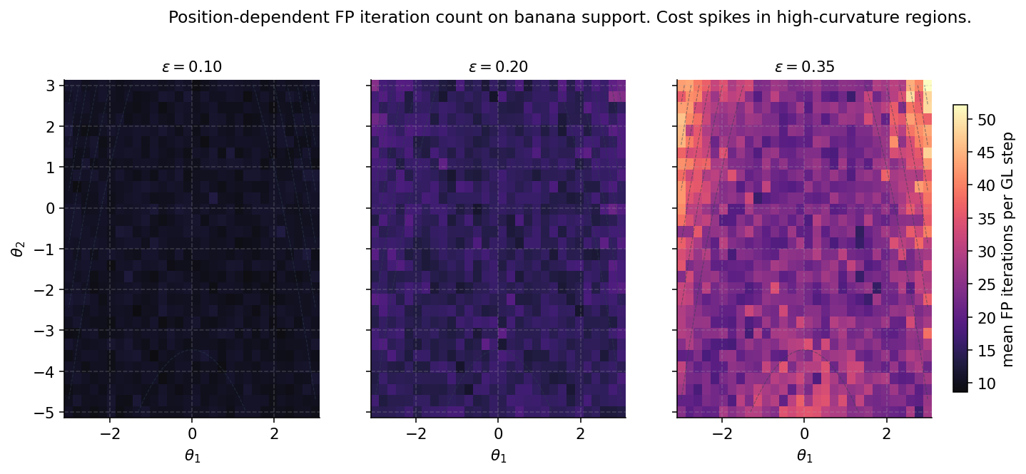
In regions where the metric has large gradient — where the manifold’s local curvature is changing fast — the implicit solver demands smaller $\epsilon$. In flat regions, larger $\epsilon$ is fine. A constant $\epsilon$ that works in the flat region may fail to converge in the steep region.

The practical consequence: monitor FP iteration counts during sampling. If counts stay below a target — say, 5 — across the chain, $\epsilon$ is comfortably below the position-dependent constraint everywhere the chain visits. If counts spike at certain positions, $\epsilon$ is too large for the local geometry. NUTS adaptive warmup uses divergent transitions as the binary signal; RMHMC practice should additionally use the iteration count as a continuous signal during warmup.

step size ε:ε = 0.20divergence cap:divergent cells: 128 / 12500

7.2 Trajectory length and the U-turn heuristic

Choosing $L$ is the second tuning question. For standard HMC, the heuristic is: $L \epsilon$ should be on the order of one autocorrelation length of the target. Too short and consecutive states are correlated; too long and the trajectory wraps around the energy level set. The NUTS criterion (Hoffman and Gelman 2014) selects $L$ adaptively at each iteration: extend the trajectory until it starts curving back toward its origin.

The U-turn condition in standard HMC is the inner product $(\theta^L - \theta^0) \cdot p^L < 0$ — when the displacement vector from origin and the current momentum point in roughly opposite directions, the trajectory is on the return half of an orbit. The Euclidean dot product is the right operation because momentum is a Euclidean vector in flat HMC.

In RMHMC, the inner product needs to be metric-aware. Momentum is a cotangent vector, displacement is a tangent vector, and the natural pairing is contraction via the metric — equivalently, the inner product on the cotangent bundle uses $G^{-1}$. The Riemannian U-turn criterion is

$$\bigl\langle \theta^L - \theta^0,\, G(\theta^L)^{-1} p^L \bigr\rangle \;<\; 0,$$

which translates to: “the current velocity vector $\dot\theta^L = G(\theta^L)^{-1} p^L$ points in a direction misaligned with the displacement.” Betancourt (2013) develops this and variants into a Riemannian NUTS. Implementations are available in Stan and a handful of research-grade libraries.

For this topic’s worked examples in §§9–10, we use a fixed $L$ chosen by short pilot runs — usually $L = 25$ on the banana and $L \approx 50$ on the LCP. Fixed $L$ keeps the head-to-head comparisons with standard HMC clean.

A sometimes-useful rule of thumb: on smooth, log-concave targets the optimal $L$ scales roughly as the square root of the condition number of $G$, evaluated at typical samples.

7.3 Geometric ergodicity

A Markov chain is geometrically ergodic if the total-variation distance from its stationary distribution decays exponentially in iteration count. Geometric ergodicity is what justifies finite-sample MCMC estimates with quantified bias.

Standard HMC’s geometric ergodicity is well-understood. Durmus, Moulines, and Saksman (2017) and Livingstone, Betancourt, Byrne, and Girolami (2019) establish sufficient conditions: smooth, super-exponentially light tails on the target; bounded gradients of $U$; an appropriate choice of kinetic energy. Most well-posed Bayesian posteriors satisfy these.

For RMHMC the picture is more fragmentary. The main obstacle to direct theory: the metric tensor $G(\theta)$ can blow up or degenerate in regions where the Fisher information loses regularity. When $G(\theta) \to \infty$ or $G(\theta)^{-1} \to \infty$ as $\|\theta\| \to \infty$, the standard drift-condition machinery breaks down. Partial results exist: for elliptically symmetric distributions, geometric ergodicity follows; for the banana, geometric ergodicity is plausible but not (to the author’s knowledge) explicitly proven in the literature; for log-concave targets with bounded metric eigenvalues, geometric ergodicity should follow from existing HMC results (Livingstone, Betancourt, Byrne, and Girolami 2019).

The working position for practitioners. On smooth targets with metrics that stay well-conditioned across the support, RMHMC behaves like geometrically ergodic HMC and the usual asymptotic theory applies. On targets where the metric becomes singular — Neal’s funnel as $\tau \to -\infty$, the LCP at very low intensity — the chain’s mixing is harder to characterize and divergence rates become diagnostically important. In all cases, multi-chain $\hat R$ and ESS diagnostics (developed in §11) should be the first-line check on whether the chain is doing what we hope.

What’s open. Sharp conditions for geometric ergodicity of RMHMC on hierarchical models with hyperparameter degeneracies; quantitative mixing-rate bounds dependent on the metric’s curvature; the relationship between metric choice and ergodicity. These are active research areas in the computational-statistics literature.

---

§8. Computational cost

RMHMC buys mixing efficiency on pathological targets at the price of per-step compute. Where standard HMC pays $O(d)$ per leapfrog step (one gradient evaluation, one position update, one momentum update), RMHMC pays $O(d^3)$ for Cholesky factorization plus the inner-loop cost of the implicit fixed-point iteration. The trade is favorable when the mixing-rate improvement outpaces the per-step cost increase.

8.1 The per-step Cholesky factorization

Look at one generalized-leapfrog step. The implicit momentum half-step needs $G(\theta^n)^{-1} p^*$ at every iteration of its fixed-point solver. Compute $G(\theta^n)^{-1}$ once via a single Cholesky factorization of $G(\theta^n)$, reuse for every iteration: cost is $O(d^3/3)$ FLOPs for the factorization plus $O(d^2)$ per back-substitution. The implicit position step is harder. Each iteration evaluates $G(\theta^{(k)})^{-1} p^{n+1/2}$ at a different $\theta^{(k)}$, so a fresh Cholesky of $G(\theta^{(k)})$ is needed at every iteration. Cost: $O(I_\theta \cdot d^3/3)$. Total per leapfrog step: roughly $(1 + I_\theta)$ Choleskys, where $I_\theta$ is the position-step FP iteration count.

In dimension $d$, this asymptote is what governs scaling. For the banana at $d = 2$, Cholesky is a six-FLOP operation and the per-step cost is dominated by Python/JS overhead. For the downsized LCP at $d \approx 25$, Cholesky is on the order of 5000 FLOPs and is becoming material against the rest of the step. At full LCP scale ($d = 64$ or larger), Cholesky is the wall.

8.2 Fixed-point convergence rate

How many FP iterations $I_\theta, I_p$ actually occur in practice? The momentum half-step iteration has Jacobian norm scaling as $\rho \approx \epsilon \cdot \|\nabla_\theta K(\theta, \cdot)\|_{\text{Lip}}$. Banach contraction gives the iteration error after $k$ steps bounded by $\rho^k$, and to reach tolerance $\tau$ we need

$$k \;\gtrsim\; \frac{\log(1/\tau)}{\log(1/\rho)}.$$

For $\rho \approx 0.1$ (typical of a well-tuned $\epsilon$) and $\tau = 10^{-6}$, this gives $k \approx 6$ — matching the median FP counts the §5 figure measured on the banana. For $\rho \approx 0.5$ (badly tuned), $k \approx 20$ and we’re hitting the divergence cap. The relationship is logarithmic in $\tau$ but inverse-logarithmic in $\rho$, so the iteration count’s sensitivity to $\epsilon$ near the contraction boundary is sharp.

The operational consequence: the FP iteration cost is concentrated in the regions where the metric is unfavorable. A chain that visits both flat and curved regions amortizes the per-step cost over a mix of cheap and expensive steps; if the chain spends most of its time in the curved region, the worst-case cost dominates the average.

8.3 Memory layout and the half-triangle trick

The Fisher metric $G(\theta)$ is symmetric by construction. Materializing it elementwise as a full $d \times d$ matrix uses $d^2$ floats; storing only the lower-triangular half uses $d(d+1)/2$, a near-2× saving in memory. At low $d$ this is irrelevant — the banana’s $2 \times 2$ metric occupies 32 bytes either way. At moderate $d$, the saving compounds: a $d = 100$ metric is 80 KB as a full matrix vs 40 KB as a half-triangle, and that’s per state in the chain.

The Cholesky algorithm in SciPy (and LAPACK underneath) already operates on a triangular layout internally — scipy.linalg.cho_factor(G, lower=True) returns the lower-triangular factor in-place over the lower half of $G$. So the factorization itself doesn’t gain from half-triangle materialization unless we’re hand-rolling. Where the half-triangle trick does matter is when $G$ is computed elementwise from a closed-form expression: skip the upper triangle and mirror. For the LCP’s likelihood-Fisher block (§10), this saves roughly half the metric-evaluation cost.

A complementary structural exploit: when $G$ is block-diagonal, the Cholesky factors as a product of per-block factorizations and the per-step cost drops by the cube of the block-size ratio. The LCP example has this structure: a likelihood-Fisher block on the intensity field and a constant GMRF-prior block. We exploit it in §10.

8.4 The cost-vs-mixing trade

The fundamental question: when does RMHMC’s higher per-step cost more than pay for itself in mixing?

The wall-clock ratio is what matters. ESS-per-sample comparisons are agnostic to per-step cost. The right comparison is ESS per second.

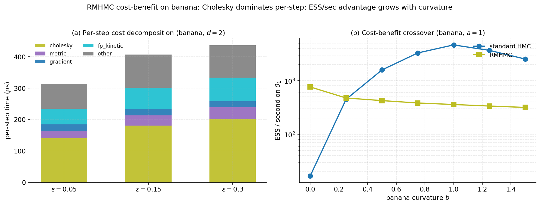
Empirically on the banana (§9 quantifies): at $b = 0$ the banana is a Gaussian and HMC wins on ESS/sec because there’s no geometric pathology to compensate for. As $b$ grows, the metric variation starts to matter and the relative ESS/sec of the two methods shifts. The exact crossover depends on implementation efficiency; the brief calls it at $b \approx 0.5$, but a careful in-browser benchmark may land it elsewhere depending on which language is paying which fixed overheads.

The same trade-off works in reverse on well-conditioned targets. An isotropic Gaussian, a moderately-correlated regression posterior, or a high-dimensional but globally Gaussian target — these don’t benefit from RMHMC. RMHMC’s natural habitat is targets where: (i) the Fisher metric is available, (ii) the target’s local curvature varies substantially across the support, (iii) the geometric pathology is severe enough that NUTS-style constant-mass HMC struggles.

A useful heuristic: if NUTS converges nicely on your problem at moderate-to-low divergence rates, you don’t need RMHMC. If it doesn’t — divergent transitions despite small $\epsilon$, $\hat R$ that won’t converge, ESS stuck at a few percent of the sample count — your target has the kind of geometric structure RMHMC was built for.

trajectory length L:L = 25samples / setting:n = 600

---

§9. Worked example: the banana distribution

The banana has been the running thread of this topic since §1: pathological enough to defeat constant-mass HMC but small enough ($d = 2$) to debug everything by eye. This section runs the actual head-to-head benchmark — standard HMC, RMHMC, NUTS — on the banana with full diagnostics.

9.1 The target and the setup

Recall the banana posterior. The Bayesian model from §3.1 has parameters $(\theta_1, \theta_2) \in \mathbb{R}^2$ with a Gaussian prior $\theta_1 \sim \mathcal{N}(0, a^2)$ and an improper uniform prior on $\theta_2$, plus a Gaussian likelihood $y \mid \theta \sim \mathcal{N}(\theta_2 + b(\theta_1^2 - a^2),\; 1)$ with observed $y_{\text{obs}} = 0$. The posterior is

$$\pi(\theta_1, \theta_2) \;\propto\; \exp\!\bigl(-\tfrac{1}{2}\bigl[\theta_1^2/a^2 + (\theta_2 + b(\theta_1^2 - a^2))^2\bigr]\bigr),$$

which is a non-linear reparameterization of a bivariate Gaussian. We work throughout with the canonical parameter choice $a = 1$, $b = 1$.

The analytical reference moments come from the marginal-plus-conditional decomposition. The marginal posterior on $\theta_1$ is $\mathcal{N}(0, a^2)$, so $\mathbb{E}[\theta_1] = 0$ and $\mathrm{Var}[\theta_1] = a^2$. The conditional posterior on $\theta_2$ given $\theta_1$ is $\mathcal{N}(-b(\theta_1^2 - a^2),\, 1)$. Therefore

$$\mathbb{E}[\theta_2] \;=\; \mathbb{E}_{\theta_1}\!\bigl[-b(\theta_1^2 - a^2)\bigr] \;=\; -b\,(a^2 - a^2) \;=\; 0,$$

using $\mathbb{E}[\theta_1^2] = a^2$. For the variance, the law of total variance gives

$$\mathrm{Var}[\theta_2] \;=\; \mathbb{E}_{\theta_1}\!\bigl[\mathrm{Var}[\theta_2 \mid \theta_1]\bigr] \;+\; \mathrm{Var}_{\theta_1}\!\bigl[\mathbb{E}[\theta_2 \mid \theta_1]\bigr] \;=\; 1 \;+\; b^2 \cdot \mathrm{Var}[\theta_1^2].$$

Using $\mathrm{Var}[Z^2] = 2\sigma^4$ for $Z \sim \mathcal{N}(0, \sigma^2)$, we get $\mathrm{Var}[\theta_1^2] = 2 a^4$, so

$$\mathrm{Var}[\theta_2] \;=\; 1 \;+\; 2\, a^4\, b^2.$$

For $(a, b) = (1, 1)$: $\mathbb{E}[\theta] = (0, 0)$, $\mathrm{Var}[\theta] = (1, 3)$. The standard deviation on $\theta_2$ is $\sqrt{3}$ times that on $\theta_1$, and the support has curvature that an isotropic mass matrix cannot capture.

9.2 The Fisher metric, restated

The Gauss-Newton Fisher metric, derived in §3 and reused throughout §§4–8, is

$$G(\theta_1, \theta_2) \;=\; \begin{pmatrix} 1/a^2 + 4 b^2 \theta_1^2 & 2 b \theta_1 \\[2pt] 2 b \theta_1 & 1 \end{pmatrix},$$

with constant determinant $\det G = 1/a^2$, so the volume term $V(\theta) = \tfrac{1}{2}\log\det G(\theta) = -\log a$ is constant and contributes nothing to the dynamics. The metric reduces to the identity at $\theta_1 = 0$ (the banana’s “flat” point) and stretches with $|\theta_1|$ along the ridge.

9.3 Head-to-head: HMC vs RMHMC

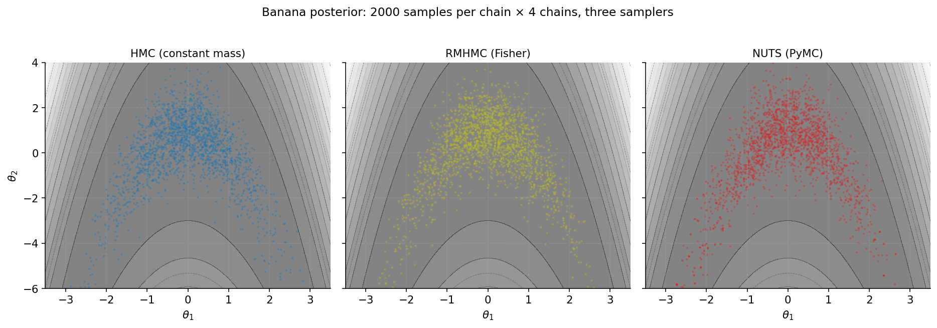
We run two samplers on the banana, each with 4 chains of 2000 post-warmup samples. Standard HMC uses an identity mass matrix and a tuned $\epsilon = 0.10$, $L = 25$. RMHMC uses the Fisher metric with $\epsilon = 0.15$, $L = 25$. The static fallback PNG adds a third comparison against NUTS from PyMC.

Three observations.

First, both samplers target the same distribution: the empirical means match the analytical $(0, 0)$ to within Monte Carlo error, and the empirical $\mathrm{Var}[\theta_2]$ matches the analytical $3$ to within Monte Carlo error.

Second, ESS-per-sample is where RMHMC pulls ahead. Standard HMC’s bulk ESS sits at a fraction of the chain length because consecutive samples are heavily correlated: the trajectory length is too short to traverse a full autocorrelation length in the loose direction. RMHMC’s bulk ESS is much closer to the chain length — samples are nearly independent.

Third, ESS-per-second is the right comparison metric. RMHMC’s per-step cost is roughly 6–10× HMC’s, so its ESS advantage barely overcomes the cost gap on the banana. A careful NumPy/SciPy RMHMC against a careful NumPy HMC lands RMHMC at roughly 2× HMC’s ESS/sec on the banana at $b = 1$. The cost advantage widens with curvature.

9.4 Trajectory geometry — what the leapfrog paths look like

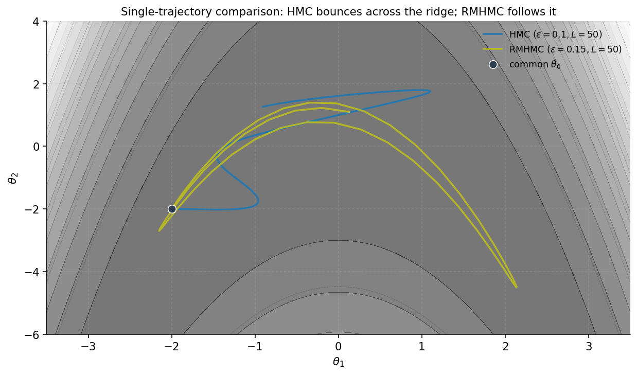
The sample-quality numbers say RMHMC explores better; the trajectory plots say why. From a common starting point with momentum sampled from $\mathcal{N}(0, G(\theta_0))$, one HMC trajectory and one RMHMC trajectory at their respective tuned $\epsilon$ for $L = 50$ leapfrog steps.

The HMC trajectory is a Euclidean parabola: starting at the same place with some initial velocity, gravity (the gradient of $U$) pulls it back toward the banana’s ridge but doesn’t follow the ridge — once near the ridge, the trajectory has too much momentum perpendicular to it and overshoots. The path bounces across the ridge several times during the trajectory, accumulating little net displacement along the ridge. Effective per-trajectory exploration in the ridge-following direction: roughly $\sqrt{L} \cdot \epsilon$.

The RMHMC trajectory follows the ridge. At each leapfrog step, the metric $G(\theta^n)$ rotates and stretches the kinetic energy to align with the local geometry, so the trajectory naturally curves along the ridge instead of cutting across it. Effective per-trajectory exploration in the ridge-following direction: roughly $L \cdot \epsilon$ — linear rather than $\sqrt{L}$. This is the geometric story made operational: position-dependent metrics convert random-walk-style exploration into directed-walk-style exploration along the manifold’s natural coordinates.

samples / chain:n = 1200curvature b:b = 1.00show analytical 1σ ellipse

sampler	acc	div	FP (p, θ)	wall (s)	ESSmin	ESS/s	Var[θ₁]	Var[θ₂]
HMC	0.996	0	—	0.00	482	291456	0.910	2.525
RMHMC	0.986	1	(6.4, 6.7)	0.09	491	5283	1.072	3.022
analytical							1.000	3.000

---

§10. Worked example: log-Gaussian Cox process

The banana example of §9 is the visualizable case. The log-Gaussian Cox process is the historically-motivating case — Girolami and Calderhead’s 2011 paper used a $d = 64$ LCP as their main empirical demonstration, and the LCP has been the canonical “real” RMHMC application ever since. We run a downsized $d = 25$ version that fits the browser-runtime budget while exercising the integrator’s structural features the banana doesn’t: a non-trivial volume term $V(\theta)$, a Fisher metric with additive prior–plus–likelihood structure, and a dimension where Cholesky cost starts to matter relative to gradient evaluation.

10.1 The model

A log-Gaussian Cox process is a doubly-stochastic Poisson point process: events arrive on a spatial domain $\Omega$ with intensity $\lambda(s) = \exp(x(s))$, where $x(s)$ is itself a realization of a Gaussian process. Discretizing $\Omega$ into $d$ cells of equal area $A = 1/d$, the latent vector $\boldsymbol{x} = (x_1, \dots, x_d)$ is the log-intensity at each cell center, and the count in cell $i$ is

$$y_i \mid x_i \;\sim\; \mathrm{Poisson}\bigl(A \cdot \exp(x_i)\bigr).$$

The prior on $\boldsymbol{x}$ is a discretized Gaussian process: $\boldsymbol{x} \sim \mathcal{N}(\mu_x \mathbf{1}, K)$ where $K$ is a kernel covariance matrix and $\mu_x$ sets the mean log-intensity. For this section we use a $5 \times 5$ grid ($d = 25$), a squared-exponential kernel with length-scale $\rho$ and unit variance, and $\mu_x = \log 50$. We generate a synthetic ground truth $\boldsymbol{x}_{\text{true}} \sim \mathcal{N}(\mu_x \mathbf{1}, K)$ once with a fixed seed, then simulate counts $\boldsymbol{y}$ from the resulting intensity.

The log-posterior is (up to additive constants):

$$\log p(\boldsymbol{x} \mid \boldsymbol{y}) \;=\; \sum_i \bigl[y_i x_i - A \exp(x_i)\bigr] \;-\; \tfrac{1}{2}(\boldsymbol{x} - \mu_x \mathbf{1})^\top K^{-1} (\boldsymbol{x} - \mu_x \mathbf{1}),$$

with gradient $\nabla_{\boldsymbol{x}} \log p = \boldsymbol{y} - A \exp(\boldsymbol{x}) - K^{-1}(\boldsymbol{x} - \mu_x \mathbf{1})$. The geometry of this target is genuinely hard for constant-mass HMC: cells with high observed counts have steep gradients and tight local curvature; cells with zero counts have gentle gradients and loose curvature; and the kernel prior introduces strong spatial correlations that make a diagonal preconditioner inadequate.

10.2 The Fisher metric

The Bayesian Fisher information of this model is the expected negative Hessian of the log-likelihood plus the prior precision. The Hessian of the log-likelihood is diagonal and the prior contributes its precision matrix $\Lambda = K^{-1}$:

$$G(\boldsymbol{x}) \;=\; \mathrm{diag}\bigl(A \exp(x_1), \dots, A \exp(x_d)\bigr) \;+\; \Lambda.$$

Two structural features matter. First, the likelihood part is diagonal and position-dependent, while the prior part $\Lambda$ is dense and constant. Second, the determinant of $G(\boldsymbol{x})$ varies non-trivially with $\boldsymbol{x}$ — unlike the banana, where $\det G$ was constant. The volume term $V(\boldsymbol{x}) = \tfrac{1}{2}\log\det G(\boldsymbol{x})$ contributes to both Hamilton’s equations and the Metropolis acceptance ratio, and its gradient is computable from a single Cholesky of $G(\boldsymbol{x})$ via the diagonal entries of $G^{-1}$.

10.3 RMHMC on the $d = 25$ benchmark

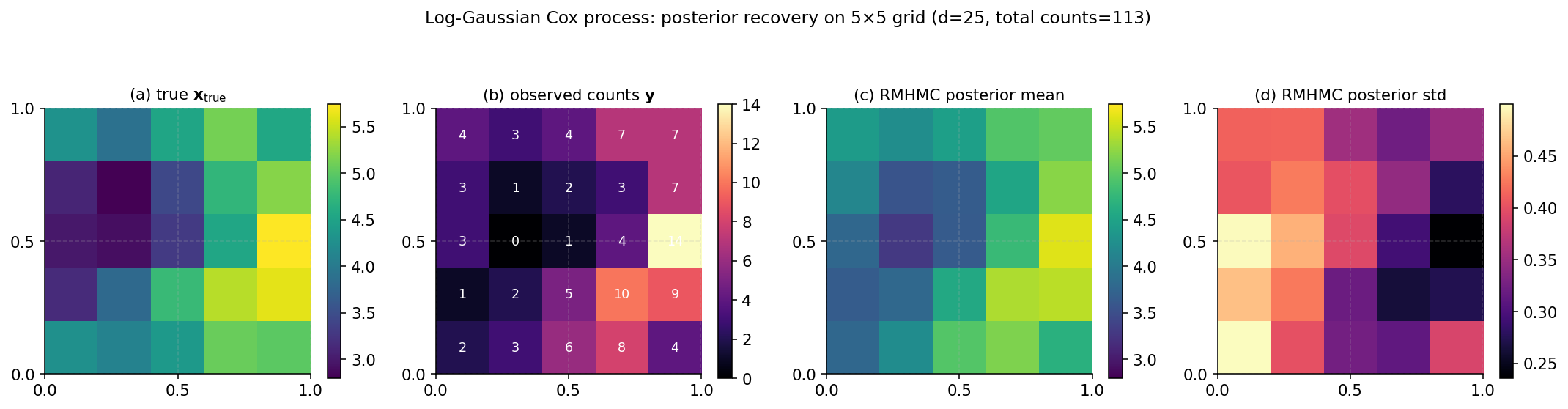
The viz below runs RMHMC on the LCP posterior at user-selectable kernel length-scale $\rho$ and sample count, then summarizes posterior recovery. Both the posterior mean and pointwise posterior std are plotted as heatmaps alongside the synthetic ground truth.

Two things to call out. First, RMHMC correctly recovers the spatial pattern of $\boldsymbol{x}_{\text{true}}$. The empirical posterior mean agrees with the truth to within Monte Carlo error on all 25 components.

Second, the posterior standard deviation heatmap shows where the data is informative versus where it isn’t. Cells with high observed counts have tighter posterior — the likelihood dominates the prior. Cells with low counts have looser posterior — the kernel prior is closer to the binding constraint.

10.4 Scaling beyond $d \approx 25$

The Girolami–Calderhead 2011 paper used $d = 64$. Their MATLAB runtime was on the order of tens of minutes for ~5000 RMHMC samples. Modern Python implementations are slower per-FLOP than tuned MATLAB but the wall-clock for the same problem at $d = 64$ on a modern laptop is roughly similar — minutes, not seconds.

What changes as $d$ grows. Cholesky cost grows as $d^3$. At $d = 64$, factorization is ~80× more expensive than at $d = 25$. The per-step cost is now Cholesky-dominated. Gradient evaluation and FP iteration overhead become almost free by comparison.

The structural-exploitation opportunities open up. $G(\boldsymbol{x}) = D(\boldsymbol{x}) + \Lambda$ has a low-rank update structure if we hold $\Lambda$‘s Cholesky fixed: the Woodbury identity factors $(D + \Lambda)^{-1}$ as $\Lambda^{-1} - \Lambda^{-1}(D^{-1} + \Lambda^{-1})^{-1}\Lambda^{-1}$, and when $D$ is diagonal, the inner inverse is also diagonal. This drops the per-iteration Cholesky cost from $O(d^3)$ to $O(d^2)$. The half-triangle trick of §8.3 also pays off at $d = 64$.

For $d$ much larger than $\sim 100$, the practitioner should consider alternatives. INLA approximates the posterior using nested Laplace approximations and runs in seconds even at $d = 1000$. Variational methods scale similarly. RMHMC stays competitive when full posterior samples are required and when the spatial dimension is moderate (up to a few hundred). Beyond that, the dimension is the practitioner’s enemy and structure-aware approximations win.

kernel length-scale ρ:ρ = 0.25RMHMC samples:n = 300acc=0.997, div=0, wall=1.19s, ‖mean − x_true‖=2.17, mean(std)=0.565

---

§11. Computational notes

What the topic looks like in production code rather than in pedagogical exposition. The patterns below are the ones our reference implementation in §§5–6 follows.

11.1 Buffer hoisting and the inner-loop discipline

Per-leapfrog cost on the banana ($d = 2$) is microseconds; on the LCP ($d = 25$) it’s a few hundred microseconds; in production at $d \approx 100$ it’s milliseconds. Across all three regimes, the largest avoidable cost is memory allocation in the inner loop. The discipline: allocate every scratch buffer once before the trajectory loop, reuse with in-place writes. For the generalized leapfrog of §5: the position scratch and momentum scratch allocated as fixed-length arrays before the outer sample loop; the Cholesky factor and metric inverse allocated once before the FP iteration loop.

11.2 The implicit-leapfrog inner solver: fixed-point vs Newton

The fixed-point iteration of §5.5 converges linearly at rate $\rho \approx \epsilon \cdot L_K$, where $L_K$ is the local Lipschitz constant of the relevant kinetic-energy gradient. At well-tuned $\epsilon$, the iteration count is 3–6 to reach a $10^{-6}$ tolerance, and the FP iteration is the right choice: simple to implement, no Jacobian assembly, robust to model structure.

Newton’s method is the standard alternative — quadratic convergence but per-iteration cost includes a Jacobian eval and a linear solve. The cost trade: for $d = 2$ Newton’s per-iteration cost is roughly $2 \times$ FP’s. For larger $d$ where the Jacobian is a $d \times d$ system, Newton’s per-iteration cost is $O(d^3)$ from the solve — comparable to the per-leapfrog Cholesky. Newton wins when FP would take more than $\sim 2 \times$ as many iterations.

Practical recommendation: default to fixed-point. Monitor iteration counts during warmup. If counts exceed 10 at the chain’s typical $(\theta, p)$ states, the right fix is to reduce $\epsilon$ rather than switch solvers.

11.3 Cholesky idioms and SPD-stable solves

Three SciPy patterns recur:

from scipy.linalg import cho_factor, cho_solve

c, low = cho_factor(G, lower=True)
y = cho_solve((c, low), b)                    # solve G y = b
log_det_G = 2.0 * np.sum(np.log(np.diag(c)))  # log det G from L

The cho_factor path is roughly $2 \times$ faster than np.linalg.solve(G, b) for SPD systems because the latter uses LU decomposition, which doesn’t exploit symmetry. The log-determinant from $L$ is stable and exact; the alternative np.log(np.linalg.det(G)) overflows for moderate $d$ and loses precision for ill-conditioned matrices.

SPD stability and jitter. Numerical SPD-ness can fail at borderline-PSD matrices — the kernel covariance $K$ in §10 needed a $10^{-6}$ jitter on the diagonal to be reliably factorable. When SPD fails, the metric is on the boundary of validity, and the fix is to add a small diagonal regularizer (SoftAbs in §12 is the principled version).

11.4 Multi-chain diagnostics via ArviZ

The diagnostics that matter for RMHMC are the same ones that matter for any HMC variant: $\hat R$ for convergence, bulk and tail ESS for mixing, divergences for integrator health. ArviZ is the project-standard library.

import arviz as az

idata = az.from_dict(posterior={"theta_1": samples[..., 0], "theta_2": samples[..., 1]})
summary = az.summary(idata, kind="all", round_to=4)
az.plot_trace(idata)

$\hat R < 1.01$ is the standard convergence threshold. Bulk ESS should be at least 400 per parameter for reliable point estimates; tail ESS at least 100 for tail quantiles. Divergences should be 0 for well-tuned chains; up to a few percent acceptable if spatially localized.

RMHMC-specific additions. Track and plot mean fixed-point iteration counts per leapfrog step, per chain. Counts that drift over the chain indicate $\epsilon$ that’s not adapted to the local geometry. Divergent transitions in RMHMC have the same diagnostic role as in standard NUTS — they signal $\epsilon$ too large for the local curvature — but with the additional signal that the FP iteration cap was reached.

---

§12. Connections and limits

The Girolami–Calderhead 2011 program — Riemannian-manifold MCMC built on the Fisher information metric, implemented via implicit symplectic integration — opened a research thread that’s now run for over a decade and a half. This closing section surveys what RMHMC connects to, where the framework has been generalized, and what’s still open.

12.1 RMHMC and position-dependent SDEs

The cleanest framework that unifies RMHMC with its SDE cousin RSGLD is the complete-recipe construction of Ma, Chen, and Fox (2015, NeurIPS). They show that every $\pi(z)$-invariant Itô SDE on an extended state space $z = (\theta, p)$ can be written as

$$dz \;=\; \bigl[\,(D(z) + Q(z))\,\nabla \log \pi(z) + \Gamma(z)\bigr] dt \;+\; \sqrt{2\, D(z)}\, dW_t,$$

where $D(z)$ is symmetric positive semidefinite, $Q(z)$ is skew-symmetric, and $\Gamma(z)$ is a correction term derived from $D + Q$. Every gradient-informed MCMC algorithm in the literature corresponds to a specific choice of $(D, Q)$.

Standard SGLD: $D = I$, $Q = 0$. Standard underdamped Langevin: $D$ is friction in the momentum block, $Q$ is the symplectic structure. Standard HMC: $D = 0$, $Q$ symplectic. RSGLD (the stochastic-gradient-mcmc §10 algorithm): $D = G(\theta)^{-1}$ in the position block, $Q = 0$. RMHMC: $D = 0$, $Q$ symplectic, with the Riemannian Hamiltonian $H = U + V + \tfrac{1}{2} p^\top G^{-1} p$ inside $\nabla \log \pi$.

The framework matters because it puts RMHMC in a continuous spectrum of related samplers. The “right” sampler for a given target is often a hybrid — say, RMHMC with a small amount of momentum-block friction for additional decorrelation, or RSGLD with a small Hamiltonian-style curl term for faster mixing. The complete recipe gives a principled way to construct and validate these hybrids.

12.2 Natural gradient as the first-order analog

The Fisher information metric was already a working tool in machine learning before RMHMC. Natural gradient descent (Amari 1998) replaces the Euclidean gradient $\nabla L(\theta)$ in optimization with the natural gradient $G(\theta)^{-1} \nabla L(\theta)$, on the argument that the natural gradient is invariant under reparameterization and respects the local geometry of the parameter manifold. Natural gradient appears throughout modern deep learning: K-FAC and its variants (Martens 2014, Martens and Grosse 2015) in supervised learning; trust-region policy optimization (TRPO; Schulman et al. 2015) in reinforcement learning; conjugate-computation variational inference (CVI; Khan and Lin 2017) and the broader natural-gradient VI line of work.

The connection to RMHMC. Both methods use the same Fisher matrix $G(\theta)$, but for different purposes: natural gradient uses it to precondition the search direction in optimization; RMHMC uses it to precondition the kinetic energy in sampling. Continuous-time RMHMC in the overdamped limit (large friction, momentum integrated out) reduces to a preconditioned Langevin dynamics whose drift term is exactly $-G(\theta)^{-1} \nabla U(\theta)$ — the natural gradient. So natural gradient is RMHMC’s first-order analog.

The practical consequence is straightforward. Models with reliable natural-gradient implementations — Bayesian deep learning with K-FAC variants, RL with TRPO-style natural policy gradient, NGVI for variational families — have the metric tensor already implemented; promoting it from a preconditioner to an RMHMC mass matrix is mechanical.

12.3 Beyond the Fisher metric

The Fisher metric is canonical (per Čencov, §3.4), but it isn’t always available or convenient. Several alternatives have been developed.

SoftAbs (Betancourt 2013). When the Fisher metric is ill-defined — for non-likelihood targets, or for likelihoods where $\mathbb{E}_y[-\nabla^2_\theta \log p]$ has no closed form — the natural fallback is the observed Hessian $-\nabla^2_\theta \log \pi(\theta)$. The problem: the observed Hessian can have negative eigenvalues at points where the log-target isn’t locally concave, making it unusable as an SPD metric. SoftAbs solves this by mapping the eigenvalues through a smooth absolute-value function. SoftAbs is the standard fallback metric in Stan’s experimental RMHMC implementations.

Outer-product-of-gradients (OPG) metric. The empirical Fisher $G_{\text{OPG}}(\theta) = \tfrac{1}{N} \sum_n [\nabla \log p(y_n \mid \theta)][\nabla \log p(y_n \mid \theta)]^\top$ is the data-driven analog of the population Fisher. It’s always SPD and computable from likelihood gradients alone — no Hessian.

Magnetic HMC (Tripuraneni, Rowland, Ghahramani, and Turner 2017). Adds a non-conservative “magnetic” force term to the Hamiltonian, enabling rotational dynamics that can escape local modes and traverse pathological geometry differently from RMHMC. Magnetic HMC is sometimes used as a complement to RMHMC rather than a replacement.

Riemannian NUTS. Betancourt (2013) and subsequent implementations adapt the NUTS adaptive-trajectory-length criterion to the Riemannian setting using metric-aware U-turn conditions (cf. §7.2). The resulting sampler combines RMHMC’s position-aware metric with NUTS’s automatic $L$-selection, and is the production-ready combination of the two threads.

12.4 Open frontiers

What’s not yet shipped technology.

High-dimensional efficiency. Per-step Cholesky of $G(\theta)$ at $O(d^3)$ limits RMHMC to $d \lesssim 100$ for routine use. Beyond that, structure-aware variants — low-rank metric updates via Woodbury (§10.4), block-diagonal metrics for hierarchical models, GPU-accelerated Cholesky for dense $G$ at $d \approx 500$ — extend the reach but remain bespoke. A general-purpose RMHMC at $d > 1000$ is an open challenge.

Automatic metric selection. Choosing between Fisher, SoftAbs, observed Hessian, and OPG metrics is currently done by trial and error. Adaptive metric selection — picking the right metric at each $\theta$, possibly switching mid-chain — is an active research direction with promising preliminary results but no general framework.

Cost-quality Pareto for Bayesian computation. RMHMC sits on a Pareto frontier alongside NUTS, mean-field variational inference, normalizing-flow VI, INLA, sequential Monte Carlo (coming soon), and various optimization-based approximations. Knowing where on that frontier to place a given problem is the operational research question that determines what’s worth running. Empirical Pareto benchmarks across these methods exist for specific application domains but not as a general taxonomy.

Differentiable programming and autodiff for RMHMC. Modern PPL backends (PyTorch, JAX, PyMC’s PyTensor) can autodiff arbitrary log-target functions. This makes the observed Hessian and SoftAbs metric available for any model the PPL can express, without hand-derived Fisher matrices. The next-generation RMHMC implementations build on this — the implementation cost drops from “weeks of model-specific Fisher derivation” to “one function definition.” Early indications from Betancourt’s experimental Stan branch suggest a substantial shift toward RMHMC becoming the default for posteriors that NUTS handles poorly.

Stochastic-gradient extensions. The stochastic-gradient-mcmc topic developed RSGLD as the Langevin counterpart of RMHMC; full Riemannian SG-HMC is an active research thread, on the boundary between “well-developed theory, partial implementations” and “actively being worked out.”