Reversible-Jump MCMC

§1. Overview and motivation

1.1 Where fixed-dimension MCMC stops working

Standard Metropolis–Hastings and Gibbs — the §26 catalog in formalStatistics: bayesian-computation-and-mcmc — presume a fixed parameter space $\Theta \subseteq \mathbb{R}^d$. The chain is a random walk on this Euclidean (or product-of-Euclidean) ambient space. As long as the target density $\pi(\theta)$ is well-defined on a fixed-dimensional support and the proposal density $q(\theta' \mid \theta)$ has a known closed form, the §26 framework gives us everything we need to construct a $\pi$-invariant chain.

Model selection breaks this presumption at the root. We have a finite or countable collection of candidate models $\{M_1, M_2, M_3, \ldots\}$ with parameter spaces $\Theta_1, \Theta_2, \Theta_3, \ldots$ — and the whole point of model selection is that $\dim(\Theta_k) \neq \dim(\Theta_{k'})$ in general. Model $M_3$ might be a five-parameter regression with three covariates; $M_7$ might be a twelve-parameter regression with ten. The Bayesian posterior we want to sample is the joint

$$p(M_k, \theta_k \mid \mathcal{D}) \;\propto\; p(\mathcal{D} \mid M_k, \theta_k)\, p(\theta_k \mid M_k)\, p(M_k),$$

which lives on the disjoint union

$$\mathcal{X} \;=\; \bigsqcup_{k} \{k\} \times \Theta_k,$$

a state space whose dimension changes as the chain moves between models. No single Euclidean ambient space accommodates the chain; no fixed-dim proposal density $q(\theta' \mid \theta)$ even has a well-defined form when source and target live in different dimensions. The change-of-variables formula — the one piece of measure theory that makes the trans-dimensional move sensible — does not appear anywhere in the §26 catalog because nothing in that catalog ever changes dimension.

The naive workaround — fix the model at its largest plausible size and trust a continuous spike-and-slab prior to push unused coefficients toward zero — does work for moderate $p$. That’s the sparse-bayesian-priors §12 setup, and it’s the lead-in this topic explicitly extends rather than re-derives. But the continuous spike-and-slab posterior concentrates mass near zero, not at zero, so we can never read off a posterior inclusion probability $p(\gamma_j = 1 \mid \mathcal{D})$ directly. For Bayes factors, posterior model probabilities, and predictive averaging — the BMA tasks of formalStatistics: bayesian-model-comparison-and-bma — we need $\gamma$ as a discrete indicator the chain visits or doesn’t. That’s the gap RJ-MCMC fills.

1.2 Two motivating pictures

Two examples will recur §-by-§ throughout the topic. We introduce both here so that every later section can point back to one or the other for a concrete instance of whatever abstraction we’re unpacking.

The variable-selection lattice. Given $p$ candidate covariates, the model space is the power set: $2^p$ subset-models indexed by binary indicators $\gamma \in \{0,1\}^p$, where $\gamma_j = 1$ iff covariate $j$ is included. Two models are neighbors if their $\gamma$ vectors differ by exactly one coordinate — one variable added or one dropped. The model space inherits a natural graph structure: the $p$-dimensional Boolean lattice, with layers indexed by cardinality $|S| = \sum_j \gamma_j$ and edges only between adjacent layers. Figure 1A draws the $p = 4$ case (16 models, 32 edges) at scale; in §9’s worked example we run at $p = 8$ (256 models), at which scale full enumeration is still tractable and we can validate posterior inclusion probabilities exactly against an enumeration-computed gold standard.

The mixture-order question. Given a univariate dataset, how many Gaussian components do we need? Each candidate model $M_K$ has parameters $\theta_K = (\mu_1, \sigma_1^2, w_1, \ldots, \mu_K, \sigma_K^2, w_K)$ — a $(3K-1)$-dimensional space (the $-1$ comes from the simplex constraint $\sum_j w_j = 1$). As $K$ grows, dimension grows by 3 per added component. RJ-MCMC moves between $K$ and $K \pm 1$ by splitting one component into two (dimension up by 3) or merging two into one (dimension down by 3), with auxiliary variables that parameterize how the split-or-merge happens. Figure 1B shows the canonical Galaxy dataset (Roeder 1990, $n = 82$ velocities in km/s × $10^3$) with $K = 2$, $K = 4$, $K = 6$ candidate fits overlaid. Visually, $K = 2$ underfits the central cluster, $K = 6$ adds bumps with no real support, and $K = 3$ or $K = 4$ looks about right — but the principled posterior over $K$ requires the sampler we’re building. The numerical answer (Richardson–Green 1997 §6) is a posterior centered around $K = 3$ to $5$ depending on prior hyperparameters, and §10 reproduces this.

1.3 Why Carlin–Chib and product-space samplers don’t suffice

Before Green (1995), the standard approach to trans-dimensional Bayesian computation was the Carlin–Chib (1995) product-space sampler. The construction: define an over-parameterized chain on the Cartesian product $\Theta_1 \times \Theta_2 \times \cdots$ that always carries every model’s parameters simultaneously, plus a categorical model-index variable that selects which model’s parameters drive the likelihood at each iteration. Inactive models’ parameters are updated from “pseudo-priors” chosen by the user. Marginalizing the categorical variable recovers the posterior model probabilities; the standard Gibbs machinery handles the rest.

The construction is mathematically clean and historically important, but it has two crippling costs in practice. First, every iteration updates every model’s parameters even though only one is active, so per-iteration cost scales with the total dimension of all candidate models combined — exactly the scaling we wanted to avoid. Second, the pseudo-priors on inactive parameters have to be tuned per application to match the corresponding conditional posteriors closely enough that the categorical-variable mixing isn’t catastrophically slow; this tuning is itself a model-fitting exercise, sometimes harder than the original problem. For more than three or four candidate models, Carlin–Chib is unworkable.

Green (1995) keeps the disjoint-union state space $\mathcal{X}$ and constructs each dimension-changing move as a deterministic measurable bijection on a padded common space, with auxiliary random variables drawn only on the source side. The bijection is reversible by construction (the inverse map is the reverse move), and the trans-dimensional MH acceptance ratio that results has one new ingredient compared to fixed-dim MH: a Jacobian determinant from the change-of-variables formula on the bijection. The acceptance ratio is computationally trivial to evaluate, the move catalog is hand-engineered per problem but transparent, and the chain genuinely lives on $\mathcal{X}$ rather than on an inflated product space. RJ-MCMC subsumes Carlin–Chib and is uniformly more efficient. We mention Carlin–Chib once more, in §13’s tooling notes, and otherwise leave it to the references.

1.4 What this topic discharges

RJ-MCMC discharges three site-wide forward-pointers and closes one curriculum cluster:

• formalStatistics: bayesian-computation-and-mcmc §26.10 Rem 28 explicitly forward-pointed at RJ-MCMC as the trans-dimensional extension of the §26 MH/Gibbs catalog. §§4–7 of this topic discharge that pointer.
• formalStatistics: bayesian-model-comparison-and-bma forward-pointed at RJ-MCMC as the canonical sampler for the posterior model probabilities $p(M_k \mid \mathcal{D})$ that BMA averages over. §§9–10 discharge that pointer with worked examples.
• sparse-bayesian-priors §12.6 named RJ-MCMC as the discrete spike-and-slab workhorse for the $p > 30$ regime where Gibbs SSVS becomes prohibitive. §9 discharges that pointer by extending the continuous-spike-and-slab framework to the discrete case.

RJ-MCMC also closes the T5 specialized-sampler cluster. stochastic-gradient-mcmc handled noise-injected gradient samplers for big-data targets; riemann-manifold-hmc handled position-dependent Fisher mass matrices for pathological fixed-dim targets; sequential-monte-carlo handled annealed-target evidence estimation for hard posteriors. RJ-MCMC handles dimension-changing moves for model selection. After this topic, the T5 Bayesian-computation toolkit is structurally complete and the ML Methodology layer’s specialized-sampler cluster closes.

1.5 Roadmap

§2 names the Bayesian-model-selection target — what RJ-MCMC samples from and what it returns. §3 builds the trans-dimensional state space $\mathcal{X}$ as a geometric object with two concrete pictures (the lattice from §1.2, the dimension-stair from §1.2). §4 cites the standard MH framework and pins down exactly where it stops short. §§5–7 are the load-bearing proof triplet: the auxiliary-variable bijection (§5), reversibility (§6), detailed balance with the Jacobian factor (§7). §8 catalogs the standard moves — birth/death, split/merge, within-model updates — and writes their Jacobians out. §§9–10 run the math on real data: linear-regression variable selection at $p = 8$ (§9) and Galaxy-data mixture-order estimation up to $K_{\max} = 6$ (§10). §11 covers diagnostics specific to trans-dimensional chains. §§12–13 wrap with computational notes and connections to the rest of the site.

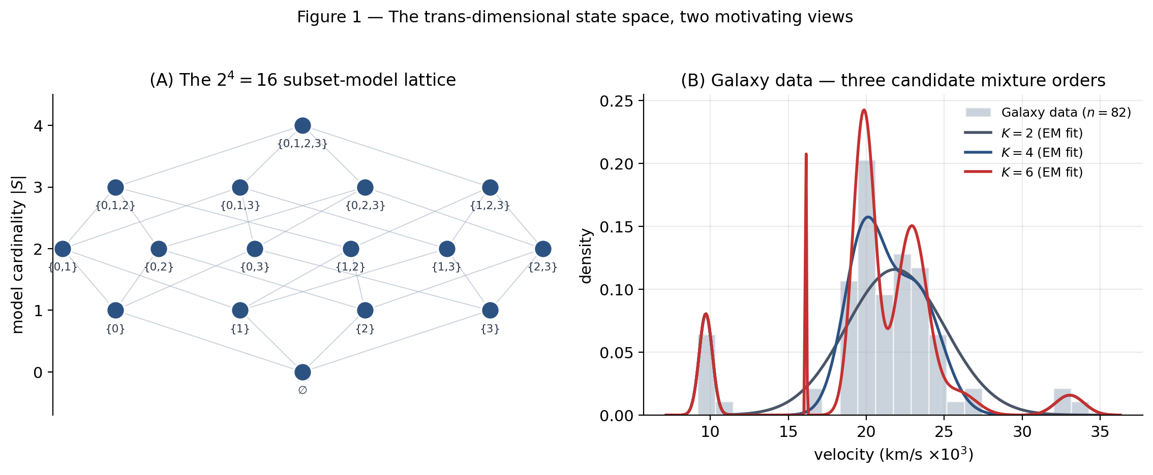
Try dragging the $p$ slider on the lattice or the $K$ slider on the Galaxy histogram below. Click a lattice node to highlight its Hamming-distance-one neighbors — the moves an RJ-MCMC add/drop catalog would propose from that state.

p = 42⁴ = 16 models

K = 3n = 82

§2. Bayesian model selection at a glance — what RJ-MCMC computes

§2 names the target. RJ-MCMC is a sampler, and like every sampler it samples from something specific. The “something specific” is the trans-model posterior $p(M_k, \theta_k \mid \mathcal{D})$ and its marginal $p(M_k \mid \mathcal{D})$, both well-known objects from formalStatistics: bayesian-model-comparison-and-bma . We re-state them here in the notation we’ll use for the rest of the topic and pin down what RJ-MCMC actually returns when a chain finishes running.

2.1 The trans-model posterior and the posterior model probability

Bayesian model selection starts from a collection of candidate models $\mathcal{M} = \{M_1, M_2, \ldots\}$, each with its own parameter space $\Theta_k$, likelihood $p(\mathcal{D} \mid \theta_k, M_k)$, and parameter prior $p(\theta_k \mid M_k)$. A separate model prior $p(M_k)$ assigns probability to each candidate. Bayes’ rule applied to the full joint gives

$$p(M_k, \theta_k \mid \mathcal{D}) \;=\; \frac{p(\mathcal{D} \mid \theta_k, M_k)\, p(\theta_k \mid M_k)\, p(M_k)}{p(\mathcal{D})},$$

with normalizer

$$p(\mathcal{D}) \;=\; \sum_{k'} p(M_{k'}) \int_{\Theta_{k'}} p(\mathcal{D} \mid \theta_{k'}, M_{k'})\, p(\theta_{k'} \mid M_{k'})\, d\theta_{k'}$$

— a sum over models, each summand an integral over that model’s parameter space. The normalizer is finite when each per-model marginal likelihood is finite and $\sum_k p(M_k) = 1$ (the model prior is proper), which is the regularity setting throughout the topic.

Marginalizing $\theta_k$ out of the joint defines the posterior model probability

$$p(M_k \mid \mathcal{D}) \;=\; \frac{p(\mathcal{D} \mid M_k)\, p(M_k)}{p(\mathcal{D})}, \qquad p(\mathcal{D} \mid M_k) \;=\; \int_{\Theta_k} p(\mathcal{D} \mid \theta_k, M_k)\, p(\theta_k \mid M_k)\, d\theta_k,$$

where $p(\mathcal{D} \mid M_k)$ is the marginal likelihood (or model evidence) for $M_k$ — the same object SMC §8 estimated unbiasedly via $\widehat{Z}_T$, here viewed one model at a time.

RJ-MCMC samples directly from the trans-model joint on the disjoint union $\mathcal{X} = \bigsqcup_k \{k\} \times \Theta_k$. The estimator for posterior model probabilities is the time-fraction estimator:

$$\widehat{p}(M_k \mid \mathcal{D}) \;=\; \frac{1}{N - N_{\text{burn}}} \sum_{t = N_{\text{burn}} + 1}^{N} \mathbb{1}\!\left[M^{(t)} = M_k\right].$$

This is the trans-dimensional analog of the fact that fixed-dim MCMC estimates a posterior mean by averaging the parameter trace — “fraction of post-burn-in time in state $A$” is just the Monte Carlo estimate of $\mathbb{E}_\pi[\mathbb{1}[\cdot \in A]] = \pi(A)$. We never compute any individual $p(\mathcal{D} \mid M_k)$; the sampler returns posterior model probabilities directly, and posterior summaries within each model (conditional means, credible intervals for $\theta_k \mid M_k, \mathcal{D}$) come from averaging over only the iterations where $M^{(t)} = M_k$. We’ll return to this within-model vs. across-model decomposition in §11.

2.2 Bayes factors, model priors, and the binomial multiplicity

The Bayes factor comparing $M_k$ to $M_{k'}$ is the ratio of marginal likelihoods,

$$B_{kk'} \;=\; \frac{p(\mathcal{D} \mid M_k)}{p(\mathcal{D} \mid M_{k'})} \;=\; \frac{p(M_k \mid \mathcal{D})\, /\, p(M_{k'} \mid \mathcal{D})}{p(M_k)\, /\, p(M_{k'})},$$

the multiplicative factor by which $\mathcal{D}$ updates the prior odds of $M_k$ over $M_{k'}$. Bayes factors are prior-free in the parameters (the $\theta_k$ are integrated out) but not prior-free in the model — they depend on the parameter priors $p(\theta_k \mid M_k)$ inside each marginal likelihood. This is the well-known Lindley–Bartlett sensitivity: a flat parameter prior over a wide range makes $p(\mathcal{D} \mid M_k)$ tiny relative to a prior concentrated near the true value, biasing the Bayes factor against the larger model. The conjugate $g$-prior of Zellner (1986) and its hyper-$g$ refinements (Liang et al. 2008) are the standard fix in the regression setting and what §9 uses.

The model prior $p(M_k)$ is rarely well-chosen as uniform-over-models in the variable-selection setting. With $2^p$ models indexed by $\gamma \in \{0,1\}^p$, the uniform prior $p(\gamma) = 2^{-p}$ assigns probability $\binom{p}{k}/2^p$ to “the model has cardinality exactly $k$,” which is binomially concentrated around $k = p/2$. For genuinely sparse problems (true cardinality $k^\star \ll p/2$) this puts vanishing mass on the right neighborhood. The standard fix, the Scott–Berger (2010) multiplicity-correction prior, makes the model size $|S|$ uniform on $\{0, 1, \ldots, p\}$:

$$p(\gamma) \;\propto\; \binom{p}{|\gamma|}^{-1} \cdot p(|\gamma|), \qquad p(|\gamma|) \;=\; \frac{1}{p+1}.$$

The $\binom{p}{|\gamma|}^{-1}$ factor exactly cancels the multiplicity of models at each cardinality, so a posteriori the model size is driven by the data, not by the combinatorial geometry of the lattice. §9 uses Scott–Berger; you’ll see $\binom{p}{|\gamma|}$ appear directly in the log-prior code via scipy.special.gammaln.

For the mixture-order setting (§10), the analog is much simpler: $p(K) \propto 1$ on $\{1, \ldots, K_{\max}\}$, or a truncated Poisson with rate fit to elicited prior beliefs. Richardson–Green (1997) used $\mathrm{Poi}(1)$ truncated to $\{1, \ldots, 30\}$, which puts most mass on $K \in \{1, 2, 3, 4, 5\}$ — broad enough to let the Galaxy data drive the answer but with built-in Occam-style preference for parsimony.

2.3 Why we sample instead of integrate

At small $p$ — say $p \leq 15$, so $|\mathcal{M}| \leq 32{,}768$ — with conjugate priors that admit closed-form marginal likelihoods, full enumeration of $\{p(\mathcal{D} \mid M_k) : M_k \in \mathcal{M}\}$ is feasible. Every posterior model probability can be computed exactly, no sampling required. §9 exploits exactly this fact: it runs the $p = 8$ variable-selection demo at a scale where the 256-model enumeration is the gold standard, and uses the enumerated posterior to validate RJ-MCMC’s output. Whenever enumeration is feasible, do it — RJ-MCMC then exists to convince yourself the sampler works, not to do new computation.

At $p = 30$, $|\mathcal{M}| = 2^{30} \approx 10^9$; at $p = 50$, $|\mathcal{M}| = 2^{50} \approx 10^{15}$. Even at one marginal-likelihood evaluation per microsecond — roughly an OLS fit plus a log-Gamma normalization — enumeration at $p = 30$ takes about 17 minutes and at $p = 50$ takes about 35 years. Genomic-scale variable selection routinely sits at $p$ in the thousands; enumeration is hopeless. The exponential wall is visible in Figure 2A.

For the mixture-order problem the obstruction is different but converges to the same conclusion. Even at modest $K_{\max} = 10$, the marginal likelihood $p(\mathcal{D} \mid M_K)$ is not closed-form under the weakly informative priors Richardson–Green (1997) recommend (those priors are deliberately non-conjugate to keep the prior data-independent). Each per-$K$ evidence then requires its own numerical-integration job — bridge sampling, AIS, SMC, or nested sampling — which is itself a substantial sampler-tuning exercise. Running 10 separate evidence estimators to compare 10 candidate $K$ values is wasteful when a single RJ-MCMC run on the trans-dimensional space estimates all 10 posterior probabilities simultaneously, with computation shared across model orders via the split/merge move catalog (§10).

The RJ-MCMC bargain. Instead of one numerical-integration job per model, one sampler over the trans-dimensional space that visits each model in proportion to its posterior probability. The acceptance ratio handles the per-step bookkeeping including the Jacobian determinant (§7); the time-fraction estimator handles the posterior model probabilities (§2.1). Sampler tuning is harder — auxiliary-variable proposals, move-catalog mixing, between-model jump acceptance rates — and §§8 and 11 will spend serious time on it. But the result is a single chain whose summary statistics give us everything the model-selection question asked for.

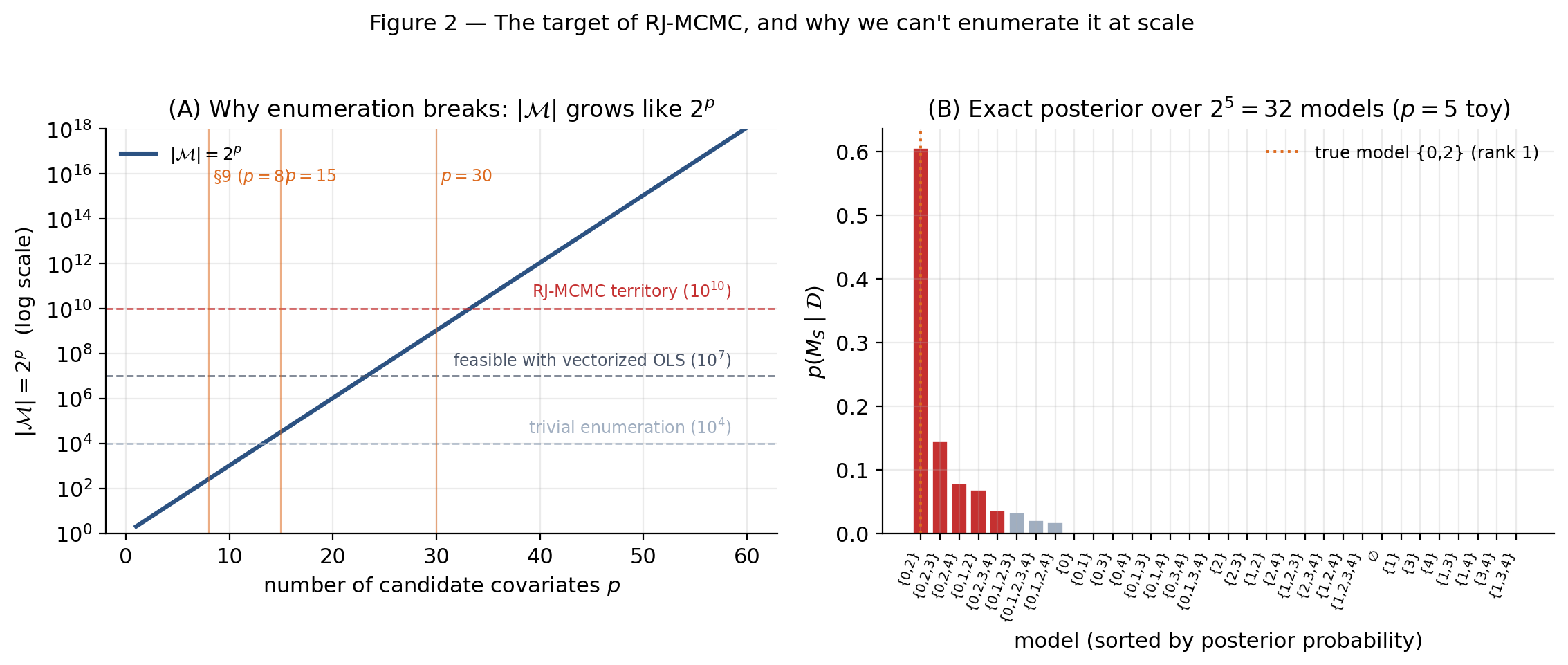
Drag the $p$ slider on the left panel to see how the enumeration wall scales; the right panel re-simulates a toy regression dataset at the chosen $p$ and re-enumerates its posterior.

p = 5

Toy regression at p = 5, n = 80, σ = 0.5 — enumerated under g-prior + Scott–Berger.

§3. The trans-dimensional state space

Before we put a Markov chain on $\mathcal{X}$, we need to look at what $\mathcal{X}$ actually is as a geometric and measure-theoretic object. The whole reason RJ-MCMC needs new machinery — auxiliary variables, Jacobian determinants, a re-derived detailed-balance condition — is that $\mathcal{X}$ is not a single Euclidean space. It’s a disjoint union of pieces of different dimensions, glued together at their boundaries by the moves we’ll eventually let the chain take. §3 makes that geometric picture precise.

3.1 The disjoint union and its measure

Formally, the trans-dimensional state space is

$$\mathcal{X} \;=\; \bigsqcup_{k \in \mathcal{K}} \{k\} \times \Theta_k,$$

where $\mathcal{K} = \{1, 2, \ldots, K_{\max}\}$ (or any countable index set) is the model index set and each $\Theta_k \subseteq \mathbb{R}^{d_k}$ is the parameter space of $M_k$, with dimension $d_k = \dim(\Theta_k)$. A point in $\mathcal{X}$ is a pair $(k, \theta_k)$: a model index and a parameter vector whose dimension depends on which model we’re in. Two points with different model indices are distinct points in $\mathcal{X}$ even if their continuous coordinates look related — there is no canonical embedding of $\Theta_3$ inside $\Theta_4$ that lets us pretend they live in the same Euclidean space.

The natural sigma-algebra $\mathcal{F}$ on $\mathcal{X}$ is the disjoint sum of the per-fiber Borel sigma-algebras: a set $A \subseteq \mathcal{X}$ is in $\mathcal{F}$ iff for every $k$, the slice $A_k = \{\theta_k \in \Theta_k : (k, \theta_k) \in A\}$ is Borel in $\Theta_k$. This is exactly the sigma-algebra one would get by treating $\mathcal{X}$ as the topological coproduct of the $\Theta_k$ and taking the resulting Borel sets.

The natural reference measure on $(\mathcal{X}, \mathcal{F})$ is the disjoint sum of (model prior × Lebesgue):

$$\mu(A) \;=\; \sum_{k \in \mathcal{K}} p(M_k) \int_{A_k} d\theta_k.$$

Here $d\theta_k$ is Lebesgue measure on $\Theta_k \subseteq \mathbb{R}^{d_k}$ and $p(M_k)$ is the model prior from §2.2. The trans-model posterior

$$\pi(k, \theta_k) \;\propto\; p(\mathcal{D} \mid \theta_k, M_k) \, p(\theta_k \mid M_k)$$

is a density with respect to $\mu$: the Radon–Nikodym derivative $d\Pi/d\mu = \pi(k, \theta_k) / Z$ exists and is what RJ-MCMC’s acceptance ratio fundamentally evaluates ratios of. As long as each fiber’s marginal likelihood is finite and the model prior sums to 1, $\mu$ is sigma-finite and the Radon–Nikodym machinery applies without fuss.

We’ll work with this $\mu$ as the reference throughout. The deep machinery in §§5–7 builds out why a chain whose proposal density involves both a model-index move and a dimension-changing parameter move can still be made $\mu$-symmetric.

3.2 Picture 1 — the subset-model lattice

The state space for variable selection has graph structure beyond its measure-theoretic skeleton. Each “node” — a model $M_S$ indexed by $S \subseteq \{1, \ldots, p\}$ — is connected to its Hamming-distance-one neighbors: the models that differ from $S$ by exactly one variable. The full structure is the $p$-dimensional Boolean lattice $\{0, 1\}^p$ ordered by inclusion, with edges between $\gamma$ and $\gamma'$ iff $\sum_j |\gamma_j - \gamma'_j| = 1$. Cardinality stratifies the lattice into $p + 1$ layers, with layer $k$ holding $\binom{p}{k}$ nodes.

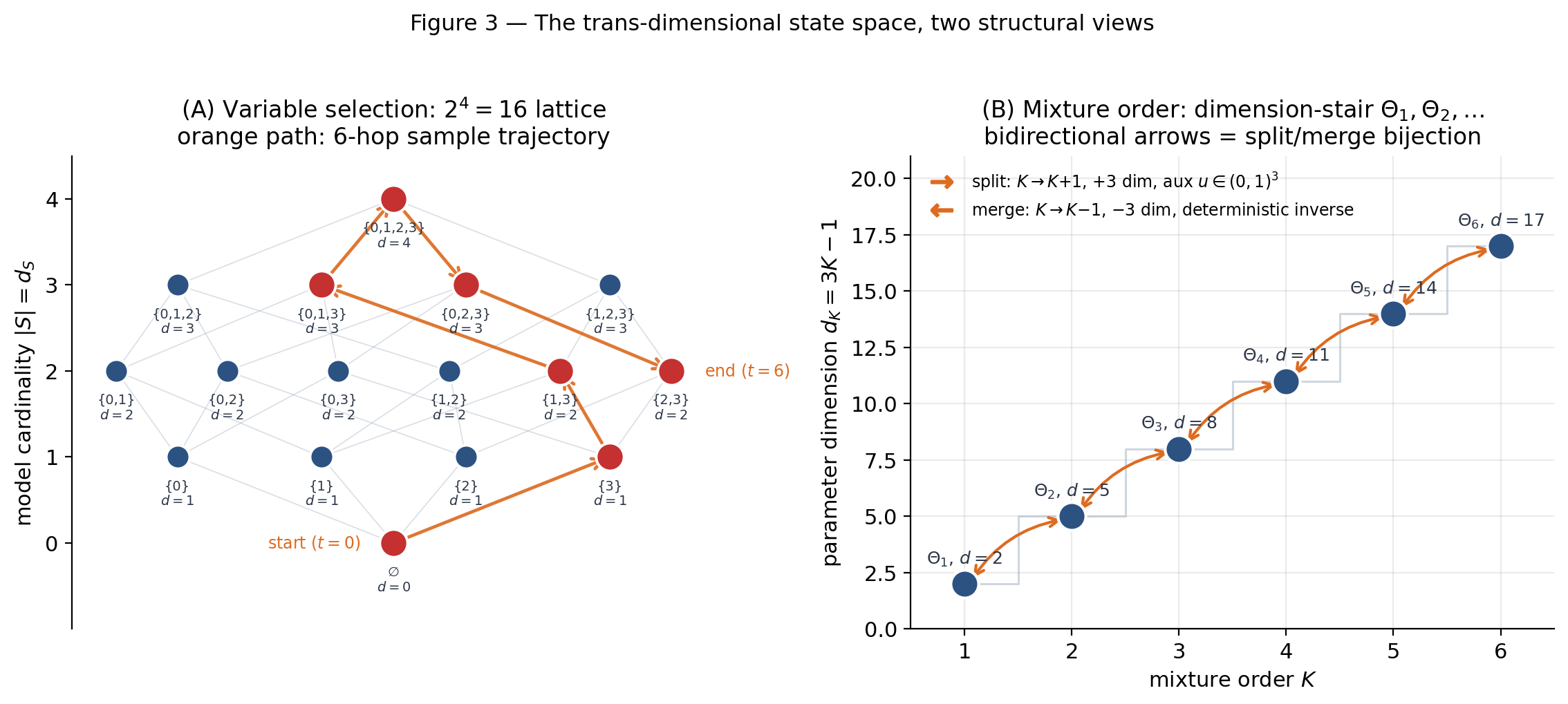
This graph structure is the natural substrate for RJ-MCMC’s move catalog. The standard add/drop catalog — propose one of the $p$ neighbors uniformly at random, accept or reject — walks along lattice edges. The chain’s state at iteration $t$ is the pair $(\gamma^{(t)}, \beta^{(t)})$, where $\gamma^{(t)} \in \{0,1\}^p$ is the current discrete coordinate (which lattice node) and $\beta^{(t)} \in \mathbb{R}^{|\gamma^{(t)}|}$ is the current continuous coordinate (the vector of coefficients for the included covariates). The discrete coordinate determines which fiber $\Theta_{\gamma^{(t)}}$ the continuous coordinate lives in. As the chain hops between lattice nodes, the dimension of $\beta^{(t)}$ changes — adding a covariate appends a dimension, dropping a covariate removes one. Figure 3A draws the $p = 4$ case with a sample 6-hop trajectory overlaid, every node annotated with its dimension $d_S = |S|$.

The geometry is sparse in a useful way: every node has exactly $p$ neighbors (not $2^p - 1$), so the move catalog at any given iteration is local in the lattice. This is what makes RJ-MCMC scale to large $p$ — proposals are cheap, even when the model space is enormous.

3.3 Picture 2 — the mixture-order dimension-stair

The mixture-order state space is even simpler topologically. Model index $K$ ranges over $\{1, 2, \ldots, K_{\max}\}$, and the parameter fiber $\Theta_K$ has dimension

$$d_K \;=\; 3K - 1 \qquad (K\ \text{means} + K\ \text{variances} + K - 1\ \text{free weights}).$$

So the dimensions are $d_1 = 2$, $d_2 = 5$, $d_3 = 8$, $d_4 = 11$, $d_5 = 14$, $d_6 = 17$: a stair-step in $K$ rising by 3 per step. Figure 3B plots this stair.

The split/merge move catalog (Richardson–Green 1997 §3.2) connects consecutive layers. From a point in $\Theta_K$, splitting one component into two yields a point in $\Theta_{K+1}$: the dimension goes up by 3. Merging two components into one yields a point in $\Theta_{K-1}$: the dimension goes down by 3. The split is not deterministic from the source state — there’s a continuum of ways to split a Gaussian component into two — so the split move draws three auxiliary variables $u_1, u_2, u_3 \in (0, 1)^3$ from Beta-distributed proposals to parameterize the split. The merge move is deterministic given which two components to combine. §10 makes this explicit; for now the picture is just dimension change ±3, plus auxiliary variables on the split side.

A complementary birth/death move catalog adds or removes an empty component, drawing the new component’s $(\mu, \sigma^2, w)$ from a prior-like proposal. The dimension change is still ±3 per move, but the new component’s parameters don’t depend on any existing component. Mixing the two catalogs (random scan between split/merge and birth/death) gives the chain more degrees of freedom to navigate the dimension stair.

One geometric caveat: each $\Theta_K$ has $K!$ symmetric copies obtained by permuting component labels — the well-known label-switching identifiability issue. The likelihood is invariant under permutations, so the posterior on $\Theta_K$ is $K!$-fold symmetric. RJ-MCMC typically samples one copy at a time (the chain rarely traverses between symmetric copies once it has settled), and we handle the symmetry post hoc when it matters for diagnostics. §11.3 returns to this.

3.4 The reference-measure problem

Here is the obstruction that motivates everything in §§5–7.

The reference measure $\mu$ from §3.1 puts Lebesgue on each fiber $\Theta_k$ separately. Within a single fiber, Lebesgue measure is the natural one — it’s what lets us write a posterior density $\pi(\theta_k \mid k)$, evaluate it, and run standard fixed-dim MCMC on $\Theta_k$. The trouble starts when we try to construct a Markov transition kernel $K\bigl((k, \theta_k), \cdot\bigr)$ that moves between fibers of different dimensions.

A standard MH proposal kernel $q(\theta' \mid \theta)$ in fixed dimension is a density with respect to Lebesgue on the target space: $q(\theta' \mid \theta) \, d\theta'$ is a probability measure on $\Theta$. When source and target have the same dimension this works fine. When source has dimension $d_k$ and target has dimension $d_{k'} \neq d_k$, there is no single Lebesgue measure that absorbs both: $d\theta_k$ and $d\theta_{k'}$ live on spaces of different dimensions and have different “units” — multiplying a coordinate by a scalar $a$ scales $d\theta_k$ by $a^{d_k}$ but $d\theta_{k'}$ by $a^{d_{k'}}$.

Concretely: if we propose moving from $\theta_k \in \Theta_k$ to $\theta_{k'} \in \Theta_{k'}$ with $d_k < d_{k'}$, the proposal must somehow produce the $d_{k'} - d_k$ “extra” coordinates that don’t have analogs on the source side. The naive fix — draw $\theta_{k'}$ from some density on $\Theta_{k'}$ directly — gives a proposal that’s not absolutely continuous with respect to any natural measure relating source and target, and the acceptance ratio that results is dimensionally inconsistent. Detailed balance then fails because we’re equating densities with respect to incompatible reference measures.

Green’s (1995) construction fixes this by working on a common higher-dimensional space. We draw auxiliary variables $u \sim q_m(u)$ on $\mathbb{R}^{d_{k'} - d_k}$ — the source side gets padded up to match the target’s dimension — and then a deterministic bijection $T_m : \Theta_k \times \mathbb{R}^{d_{k'} - d_k} \to \Theta_{k'}$ converts the padded source to the target. The proposal is now absolutely continuous on the padded space; the change-of-variables formula then relates measures on either side:

$$d\theta_{k'} \;=\; \bigl|\det J_{T_m}(\theta_k, u)\bigr| \, d\theta_k \, du, \qquad J_{T_m} \;=\; \frac{\partial T_m}{\partial(\theta_k, u)}.$$

The Jacobian determinant $|\det J_{T_m}|$ is precisely the unit-conversion factor between the natural measures on either side of the bijection. The trans-dim MH acceptance ratio includes this Jacobian as a correction factor; the resulting kernel is $\mu$-symmetric, detailed balance holds, and the chain genuinely samples the trans-dim posterior $\pi$.

This is the conceptual answer to “why is the Jacobian in the acceptance ratio.” §5 builds the auxiliary-variable construction rigorously and gives the measurability conditions (Theorem 1). §6 proves the bijection’s reversibility (Theorem 2 — the involution shortcut that makes the move catalog hand-codable). §7 puts the pieces together and derives the master acceptance ratio with full detailed-balance proof (Theorem 3). §4, immediately next, is a brief refresher on where fixed-dim MH stops short — pinning down exactly which step of the standard MH proof breaks when source and target have different dimensions.

p = 4steps = 6

K_max = 6

§4. Standard MH refresher and where it stops short

§4 names what we’re extending. The standard Metropolis–Hastings framework from formalStatistics: bayesian-computation-and-mcmc handles fixed-dimensional targets via detailed balance; §§4.1–4.2 recap just enough to fix notation. §4.3 then pins down exactly where the standard framework breaks when source and target have different dimensions — the measure-zero submanifold problem that motivates Green’s auxiliary-variable construction in §5.

4.1 The MH acceptance ratio in fixed dimension — one-line recap

For a target density $\pi(\theta)$ on $\mathbb{R}^d$ with respect to Lebesgue measure, the standard Metropolis–Hastings chain is constructed from a proposal density $q(\theta' \mid \theta)$ and the acceptance probability

$$\alpha(\theta \to \theta') \;=\; \min\!\left\{1, \; \frac{\pi(\theta')\, q(\theta \mid \theta')}{\pi(\theta)\, q(\theta' \mid \theta)} \right\}.$$

The resulting transition kernel — accept the proposal with probability $\alpha$, otherwise stay at $\theta$ — has $\pi$ as its stationary distribution under the standard regularity conditions. We cite §§26.3–26.5 of the sister-site treatment rather than re-derive.

4.2 Detailed balance as the target-invariance condition

The proof that MH preserves $\pi$ rests on detailed balance. A Markov kernel $K$ with transition density $k(\theta \to \theta')$ with respect to Lebesgue is $\pi$-symmetric iff

$$\pi(\theta)\, k(\theta \to \theta') \;=\; \pi(\theta')\, k(\theta' \to \theta)$$

for $\pi$-almost every pair $(\theta, \theta')$. Integrating both sides over $\theta$ gives $\int \pi(\theta) k(\theta \to \theta') \, d\theta = \pi(\theta')$, confirming that $\pi$ is invariant under $K$. The MH acceptance probability from §4.1 is exactly the rejection rate that makes the proposed kernel $q \times \alpha$ satisfy detailed balance.

The key technical ingredient — and the one that breaks in trans-dimensional MCMC — is that both sides of the detailed-balance equation are densities with respect to the same reference measure. Lebesgue measure on $\mathbb{R}^d$. The equation is an equality of densities on $\mathbb{R}^d \times \mathbb{R}^d$, and the standard machinery works because the densities live on the same ambient space with the same units. This is what allows us to divide both sides by $q(\theta' \mid \theta)$, take the ratio $\pi(\theta') / \pi(\theta)$, and call the resulting expression an acceptance probability.

4.3 Why the obvious “propose a model, propose its parameters” move violates detailed balance

Now try to extend MH to the trans-dimensional setting. The most efficiency-minded naive attempt: from the current state $(k, \theta_k)$, propose moving to model $k'$ with parameters $\theta_{k'} = f_m(\theta_k)$ computed deterministically from $\theta_k$ via some chosen map $f_m$. The intuition is “reuse the current parameters; only the model index changes.” Some specific instances:

• Variable-selection add-move. Propose adding covariate $j$ by setting $\beta_{\text{new}} = (\beta_{\text{old}}, 0)$ — augmenting the current parameter vector with a zero in the new slot.
• Mixture-order split-move. Propose splitting component $j$ at fixed offset $\delta$ by setting $(\mu_{j_1}, \mu_{j_2}) = (\mu_j - \delta,\, \mu_j + \delta)$ and keeping $\sigma^2_{j_1} = \sigma^2_{j_2} = \sigma^2_j$, $w_{j_1} = w_{j_2} = w_j / 2$.
• Generally: propose $\theta_{k'} = f_m(\theta_k)$ for some smooth injective map $f_m : \Theta_k \to \Theta_{k'}$ with $d_k < d_{k'}$.

The naive MH acceptance ratio would read

$$\alpha_{\text{naive}}(\theta_k \to \theta_{k'}) \;=\; \min\!\left\{1, \; \frac{\pi(k', \theta_{k'})\, \rho(k' \to k)}{\pi(k, \theta_k)\, \rho(k \to k')} \right\},$$

where $\rho(k \to k')$ is the model-index proposal probability. The expression looks fine — both $\pi$-densities are with respect to the trans-model reference measure $\mu$ from §3.1, and the ratio is dimensionless. But the framework breaks for a deeper reason that only surfaces when we ask whether detailed balance actually holds.

The injective deterministic map $f_m : \Theta_k \to \Theta_{k'}$ sends $\Theta_k$ bijectively onto the submanifold $f_m(\Theta_k) \subset \Theta_{k'}$ of dimension $d_k$. Since $d_k < d_{k'}$, the image $f_m(\Theta_k)$ has Lebesgue measure zero in $\Theta_{k'}$ — it’s a $d_k$-dimensional set inside a $d_{k'}$-dimensional ambient space, like a line inside a plane (Figure 4A draws exactly this case for $d_k = 1$, $d_{k'} = 2$). The reverse move $\theta_{k'} \to f_m^{-1}(\theta_{k'})$ is only defined when $\theta_{k'}$ happens to lie on this image submanifold — and since the submanifold has Lebesgue measure zero in $\Theta_{k'}$, the reverse-move proposal density is zero almost everywhere in $\Theta_{k'}$.

Detailed balance demands equality between forward-rate $\times$ forward-density and reverse-rate $\times$ reverse-density at the same $(\theta_k, \theta_{k'})$ pair. With the reverse-proposal density being zero almost everywhere with respect to Lebesgue on $\Theta_{k'}$, the equation is not an equality of well-defined densities — it’s an equality of mutually singular measures, and the standard MH acceptance derivation does not produce a valid kernel.

The fix is the auxiliary-variable construction. Instead of $\theta_{k'} = f_m(\theta_k)$, Green (1995) proposes

$$(\theta_{k'}, u') \;=\; T_m(\theta_k, u),$$

where $u \sim q_m(u)$ on $\mathbb{R}^{d'_m}$ is drawn from a known proposal density and $u' \in \mathbb{R}^{d''_m}$ (possibly empty) is whatever residual the move generates on the target side. The dimension-matching constraint is

$$d_k + d'_m \;=\; d_{k'} + d''_m,$$

so that $T_m$ is a smooth bijection between padded spaces of equal dimension. Its image is no longer a measure-zero submanifold — it’s a full-dimensional set in $\Theta_{k'} \times \mathbb{R}^{d''_m}$ with non-degenerate density on either side. The change-of-variables formula then relates measures on either side via the Jacobian determinant $|\det J_{T_m}|$, and detailed balance is recoverable. Figure 4B shows the simplest case: padding the 1D source $\Theta_1$ with a single auxiliary $u \sim \mathcal{N}(0, 1)$ yields a 2D joint that fills $\Theta_2$ with non-degenerate density, evading the measure-zero obstruction entirely.

This is the gap §4 names. §5 builds the auxiliary-variable construction rigorously and gives the measurability conditions in Theorem 1; §6 proves the bijection’s reversibility (Theorem 2); §7 derives the master acceptance ratio with full detailed-balance proof (Theorem 3).

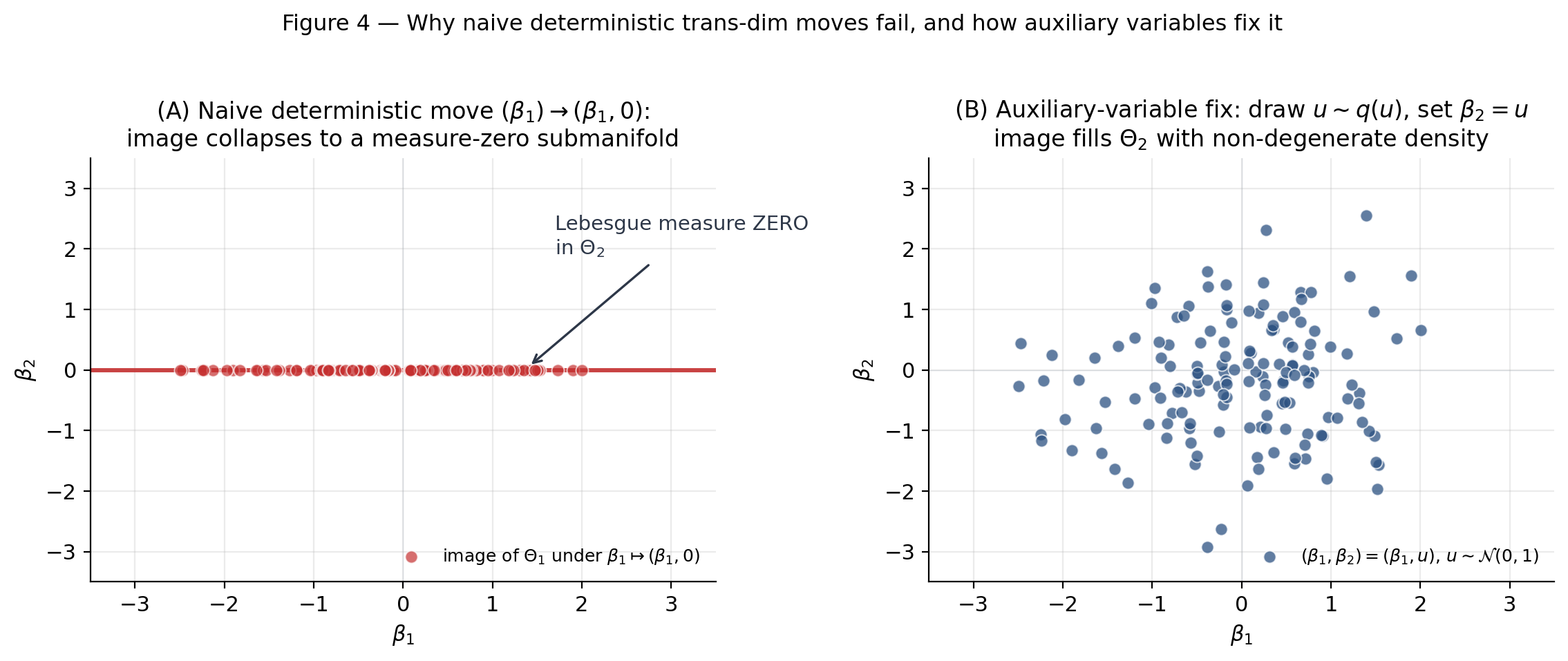
Try shrinking $\sigma_u \to 0$ and watch the auxiliary cloud collapse back onto the measure-zero line.

σ_u = 1.00

Image: line β₂ = 0 — Lebesgue measure ZERO in ℝ².

Image: scatter cloud — non-degenerate density on ℝ².

§5. The dimension-matching auxiliary-variable construction

§5 is the first of the three load-bearing proofs and the conceptual centerpiece of the topic. §4 named the obstruction — the measure-zero submanifold problem. §5 builds the fix. The construction is Green’s (1995) central trick: instead of a deterministic move $\theta_{k'} = f_m(\theta_k)$ between fibers of different dimensions, draw an auxiliary random variable $u$ on the source side, define a deterministic bijection $T_m : \Theta_k \times U_m \to \Theta_{k'} \times U'_m$ on padded spaces of equal dimension, and let the change-of-variables formula handle the rest. Theorem 1 establishes that this construction defines a well-formed proposal kernel with an explicit density on the target side, given by the source density divided by the Jacobian determinant of $T_m$.

5.1 The auxiliary-variable pair and the dimension-matching constraint

A move type $m$ in RJ-MCMC is a tuple

$$m \;=\; \bigl(k(m),\; k'(m),\; T_m,\; q_m\bigr),$$

specifying source model index $k(m) \in \mathcal{K}$, target model index $k'(m) \in \mathcal{K}$, a deterministic map $T_m : \Theta_{k(m)} \times U_m \to \Theta_{k'(m)} \times U'_m$ between padded spaces, and a probability density $q_m$ on the source-side auxiliary space $U_m \subseteq \mathbb{R}^{d'_m}$ with respect to Lebesgue. The target-side auxiliary space $U'_m \subseteq \mathbb{R}^{d''_m}$ holds whatever residual the move generates on the target side.

The dimension-matching constraint is

$$d_{k(m)} + d'_m \;=\; d_{k'(m)} + d''_m,$$

ensuring $T_m$ has domain and codomain of the same total dimension.

Three standard regimes cover all the moves we’ll need:

• Dimension-up move ($d_{k'} > d_k$). The source side is padded with $d'_m = d_{k'} - d_k > 0$ auxiliary variables; the target side has no residual, $d''_m = 0$. Example: variable-selection add-move (§9), $T_m(\beta_S, u) = \beta_{S \cup \{j\}}$ where $u \in \mathbb{R}$ becomes the new coefficient.
• Dimension-down move ($d_{k'} < d_k$). The target side has $d''_m = d_k - d_{k'} > 0$ residual auxiliary variables; the source side has no padding, $d'_m = 0$. The move is the inverse of some dimension-up move.
• Dimension-matched move ($d_{k'} = d_k$). Either $d'_m = d''_m = 0$ (deterministic same-dimension move) or $d'_m = d''_m > 0$ (auxiliary variables on both sides).

The mixture-order split-move (§10) is the canonical dimension-up move: from a state in $\Theta_K$ with $K$ components, split one component into two to land in $\Theta_{K+1}$ with $K+1$ components. The dimension change is $d_{K+1} - d_K = 3$, so $d'_m = 3$ auxiliary variables parameterize the split.

5.2 The proposal mechanism

At state $(k, \theta_k)$, the full proposal mechanism is:

1. Select a move type $m$ from the catalog with probability $j_m(k, \theta_k)$, where $\sum_m j_m(k, \theta_k) = 1$ and the sum runs over moves with source $k(m) = k$.
2. Move $m$ specifies the target model $k' = k'(m)$ and the bijection $T_m$.
3. Draw auxiliary $u \sim q_m(u)$ on $U_m$.
4. Compute $(\theta_{k'}, u') = T_m(\theta_k, u)$.
5. Accept the proposed state $(k', \theta_{k'})$ with probability $\alpha$ (derived in §7); otherwise stay.

The move-type prior $j_m(k, \theta_k)$ is the categorical distribution over moves available at the current state. It can be state-dependent — for instance, mixture-order birth/death-moves at $K = K_{\max}$ disallow births and put all mass on death-moves and within-model updates. This state-dependence is benign as long as $j_m$ is Borel-measurable in $(k, \theta_k)$.

The model-index proposal $\rho(k \to k')$ is the marginal probability that the next state’s model index is $k'$ given the current state is $k$. We keep the move type $m$ as the primitive throughout and let $\rho$ be derived.

5.3 Theorem 1 — the bijection as a measurable construction

5.4 The Jacobian determinant — what its rows and columns mean

The Jacobian matrix $J_{T_m}(\theta_k, u)$ is the $(d_{k'} + d''_m) \times (d_k + d'_m)$ matrix of partial derivatives

$$[J_{T_m}]_{ij} \;=\; \frac{\partial (T_m)_i}{\partial (\theta_k, u)_j},$$

square by dimension matching. Rows index target-side coordinates $\bigl[(\theta_{k'})_1, \ldots, (\theta_{k'})_{d_{k'}}, (u')_1, \ldots, (u')_{d''_m}\bigr]$; columns index source-side coordinates. The determinant is the signed volume-distortion factor under linearization of $T_m$ at $(\theta_k, u)$.

Numerical computation. For the variable-selection add-move (§9), $T_m$ is the identity in $(\beta_S, u)$ coordinates, so $J_{T_m} = I$ and $|\det J_{T_m}| = 1$ exactly. For the mixture-split move (§10), $T_m$ is the nonlinear Richardson–Green bijection and $|\det J_{T_m}|$ is a closed-form expression evaluated in log space via direct summation of elementary logarithms — no matrix needed. When the Jacobian has no closed form, numpy.linalg.slogdet is the right primitive (§12.2). The Jacobian determinant appears in the master acceptance ratio in §7 as the factor that makes the trans-dim Metropolis correction satisfy detailed balance.

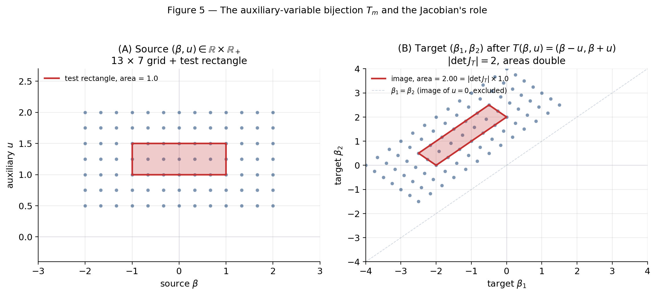
Drag $\alpha$ to scale the split: $|\det J_T| = 2\alpha$ tracks the parallelogram area. At $\alpha = 0$ the bijection degenerates to $T(\beta, u) = (\beta, \beta)$ — a measure-zero line in the target.

α = 1.00|det J_T| = 2.00

§6. Reversibility of the bijection and the involution shortcut

§6 is the second load-bearing proof. §5 built the bijection; §6 shows every move comes with a paired reverse move whose Jacobian is the reciprocal. This involution structure makes the trans-dim Metropolis correction symmetric in the move pair, which drives §7’s detailed-balance proof. Practical content: we never write down a separate “merge” or “drop” or “death” implementation. We write the dim-up direction once and the dim-down direction is computed by inverting the bijection at runtime.

6.1 The reverse move as $T_m^{-1}$

The natural candidate for the reverse of move $m$ is the move $\bar{m}$ that starts at $(k', \theta_{k'})$ and lands at $(k, \theta_k)$ by applying $T_m^{-1}$. Defining $\bar{m}$ by swapping source/target/auxiliary spaces:

• Source model $k(\bar{m}) = k'(m) = k'$.
• Target model $k'(\bar{m}) = k(m) = k$.
• Source-side auxiliary space $U_{\bar{m}} = U'_m \subseteq \mathbb{R}^{d''_m}$.
• Target-side auxiliary space $U'_{\bar{m}} = U_m \subseteq \mathbb{R}^{d'_m}$.
• Bijection $T_{\bar{m}} = T_m^{-1} : \Theta_{k'} \times U'_m \to \Theta_k \times U_m$.

The dimension-matching constraint for $\bar{m}$ is exactly the constraint for $m$ rearranged. In the standard dim-changing setting where $m$ is a dim-up move with $d'_m > 0$ and $d''_m = 0$, $\bar{m}$ is a dim-down move with $d'_{\bar{m}} = 0$ and $d''_{\bar{m}} = d'_m > 0$: the dim-down move is deterministic given the source state.

6.2 Theorem 2 — reversibility and the involution structure

6.3 The involution trick in practice

The structural message is concrete: in the move catalogs we’ll use, every dim-changing operation is naturally paired with its inverse, and we implement only one direction per pair.

Split/merge (mixture order, §10). The forward direction is split: pick a component $j$, draw $(u_1, u_2, u_3)$, apply the Richardson–Green bijection. The reverse direction is merge: pick two adjacent components, deterministically combine them via $T_m^{-1}$. The merge move requires no random ingredient — given the two components to merge, $T_m^{-1}$ produces both the merged component and the residual auxiliaries that would have generated the split.

Birth/death (mixture order, §10). Birth draws a new component from a prior-like proposal; death picks an existing component and removes it. Again the death move is deterministic given which component to remove.

Add/drop (variable selection, §9). Add draws the new coefficient $u \sim \mathcal{N}(0, \sigma_u^2)$; drop is deterministic, with the dropped value serving as the recovered auxiliary.

In each case the implementation reduces to one function per move-pair: the §9 catalog fits in about 30 lines; the §10 catalog in about 80 lines including the closed-form Richardson–Green Jacobian.

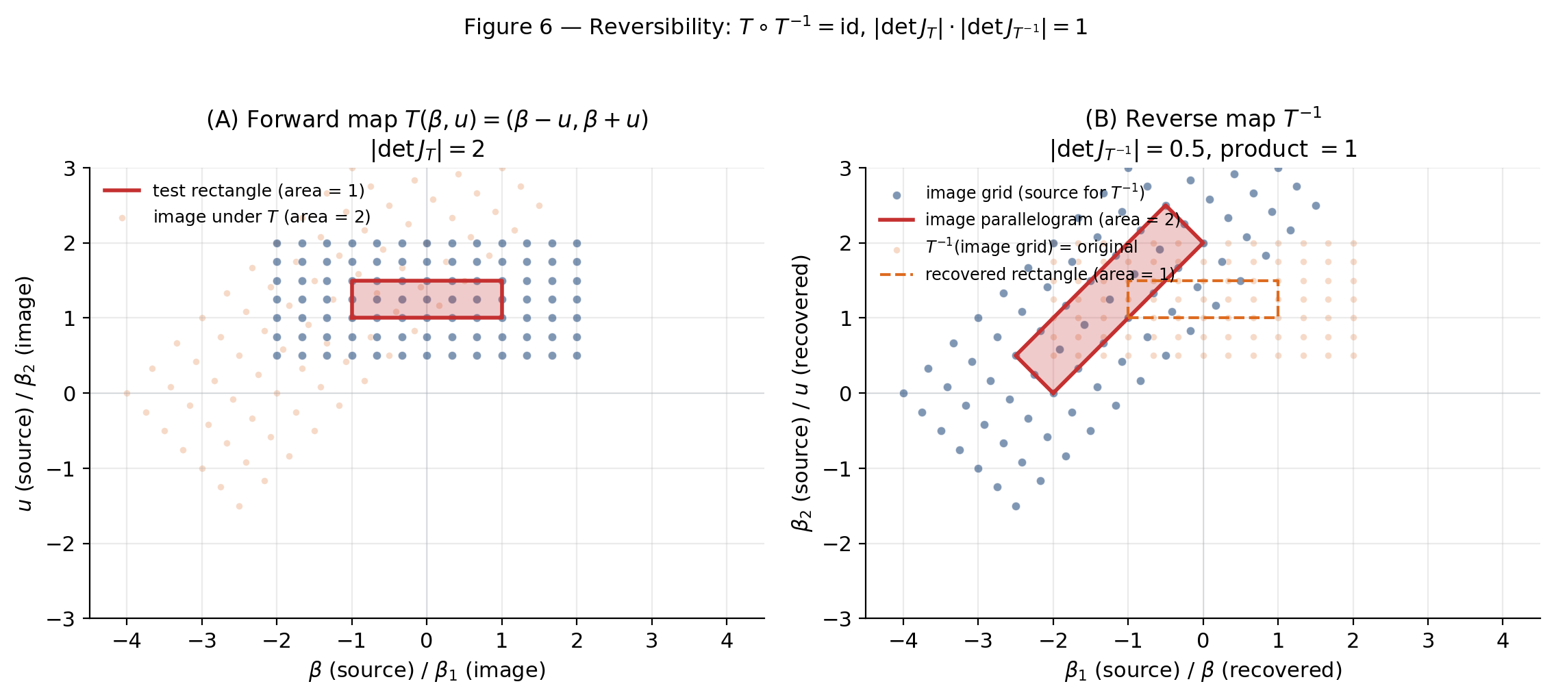
Toggle the round-trip overlay to confirm that applying $T$ then $T^{-1}$ recovers every source point — the max deviation tracks float64 machine precision.

α = 1.00Show T⁻¹∘T overlay|det J_T| · |det J_T⁻¹| = 1.000000 · max round-trip error: 2.22e-16

§7. Detailed balance with the Jacobian correction — the master acceptance ratio

§7 is the third load-bearing proof and the topic’s culminating equation. §5 built the auxiliary-variable bijection with its push-forward density (Theorem 1). §6 paired every move with its inverse and gave the Jacobian-product identity (Theorem 2). §7 assembles these into the trans-dimensional Metropolis–Hastings acceptance ratio and proves the resulting chain is $\pi$-reversible. The equation we’ll derive,

$$\boxed{\;\alpha\bigl((k, \theta_k) \to (k', \theta_{k'});\, m\bigr) \;=\; \min\!\left\{1,\; \frac{\pi(k', \theta_{k'})\, j_{\bar{m}}(k', \theta_{k'})\, q_{\bar{m}}(u')}{\pi(k, \theta_k)\, j_m(k, \theta_k)\, q_m(u)} \cdot \biggl|\det \frac{\partial T_m}{\partial(\theta_k, u)}\biggr|\right\}\;}$$

is the master acceptance ratio.

7.1 The trans-dimensional detailed-balance equation

Detailed balance in the trans-dim setting: a Markov kernel $K$ on $\mathcal{X}$ is $\pi$-reversible iff for every pair of measurable sets $A, B \subseteq \mathcal{X}$,

$$\int_A \pi(k, \theta_k)\, K\bigl((k, \theta_k), B\bigr)\, d\mu \;=\; \int_B \pi(k', \theta_{k'})\, K\bigl((k', \theta_{k'}), A\bigr)\, d\mu.$$

For the move-$m$ proposal kernel, this specializes to the pointwise equality

$$\pi(k, \theta_k)\, j_m(k, \theta_k)\, q_m(u)\, \alpha_m \;=\; \pi(k', \theta_{k'})\, j_{\bar{m}}(k', \theta_{k'})\, q_{\bar{m}}(u')\, \alpha_{\bar{m}} \cdot \bigl|\det J_{T_m}(\theta_k, u)\bigr|,$$

where the Jacobian factor on the right converts the target-side density $d\theta_{k'} \, du'$ into source-side coordinates via the change-of-variables formula. This is the trans-dim detailed-balance equation.

The new ingredient compared to fixed-dim MH (§4.1): the Jacobian factor $|\det J_{T_m}|$. In fixed-dim MH, $T_m$ is the identity, $|\det J| = 1$, and we recover the standard MH detailed-balance equation.

7.2 Theorem 3 — detailed balance with the Jacobian factor

7.3 Three special cases

Special case 1: Fixed-dim MH ($k = k'$, no auxiliary variables, Jacobian $= 1$). When the move keeps the model fixed and has no auxiliary variables, $T_m$ is the identity, $|\det J_{T_m}| = 1$, and the master ratio reduces to the standard MH acceptance ratio. RJ-MCMC contains fixed-dim MH as the no-model-change special case.

Special case 2: Identity bijection in $(\theta_k, u) \mapsto \theta_{k'}$ coordinates ($|\det J_{T_m}| = 1$). The variable-selection add-move (§9): $T_m$ literally inserts $u$ at position $j$ of the coefficient vector. $|\det J_{T_m}| = 1$ exactly. The master ratio becomes

$$A_m \;=\; \frac{\pi(S \cup \{j\}, \beta_{S \cup \{j\}})\, j_{\bar{m}}}{\pi(S, \beta_S)\, j_m\, q_m(u)}.$$

No Jacobian appears explicitly, but the structure is genuinely trans-dim — the dimension of $\beta$ changes between iterations.

Special case 3: Dimension-matched move with shared auxiliary variables ($d_k = d_{k'}$, $d'_m = d''_m > 0$, nontrivial Jacobian). An exotic case: the move keeps the model fixed but uses auxiliary variables to update $\theta_k$ via a nonlinear transformation (e.g., a reflection move in HMC-style trans-dim proposals). The Jacobian is generally nontrivial. Not used in §§9–10, but a conceptual bridge: dimension-changing isn’t the only situation where the Jacobian factor matters.

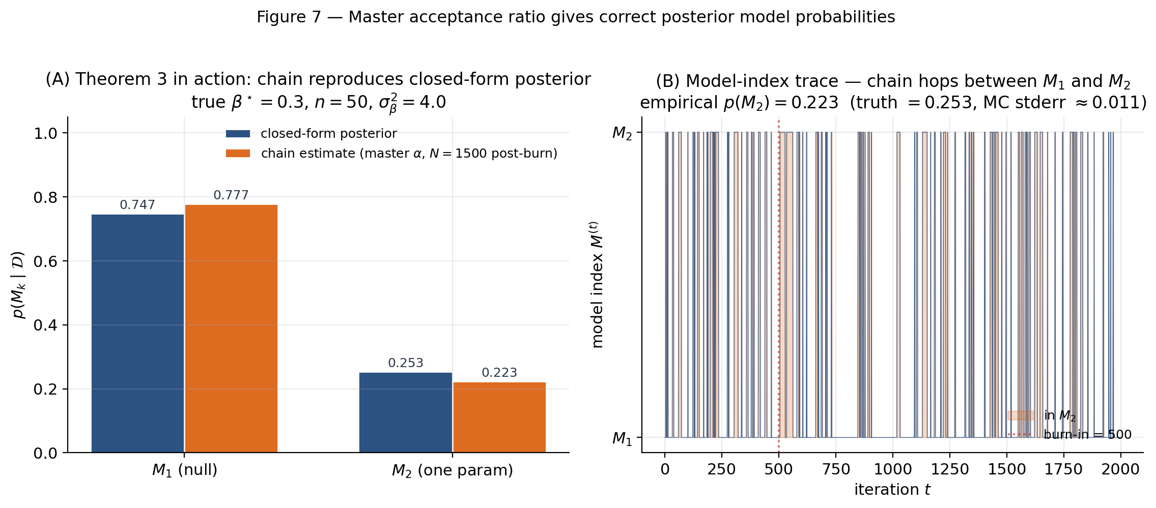
Drag $\beta^\star$ rightward to see the chain’s $P(M_2 \mid \mathcal{D})$ climb toward 1; shrink $\sigma_\beta^2$ to make the prior tighter and the Lindley–Bartlett bias against $M_2$ surface. The heavy chain recompute fires only on slider release.

β★ = 0.30

σ_β² = 4.00

n = 50

chain length T = 2000

Closed-form P(M₂|D) = 0.1084 · chain P̂(M₂|D) = 0.1093 · |error| = 0.0009 (0.1σ) · dim-acc 18.2% · within-acc 28.7%

§8. The move catalog — split/merge, birth/death, and RJ-MH

§§5–7 built the trans-dim machinery in the abstract. §8 specializes to the move catalog that actually gets implemented for the topic’s two worked examples. Each move type is fully specified by its bijection $T_m$, its auxiliary proposal $q_m$, and the Jacobian $|\det J_{T_m}|$ — all three of which we now write out in closed form.

8.1 Birth/death — the simplest dimension-changing pair

The birth move. From state $\theta_K = (\mu_1, \sigma_1^2, w_1, \ldots, \mu_K, \sigma_K^2, w_K)$, draw three auxiliary variables:

$$u_\mu \sim q_\mu(\cdot), \qquad u_\sigma \sim q_\sigma(\cdot), \qquad u_w \sim \mathrm{Beta}(1, K).$$

Typical proposals: $u_\mu \sim \mathcal{N}(\bar{y}, s_y^2)$, $u_\sigma \sim \mathrm{InvGamma}(\alpha_\sigma, \beta_\sigma)$, $u_w \sim \mathrm{Beta}(1, K)$ (Richardson–Green 1997 §4 motivates this choice). The bijection $T_m$ takes the padded source $(\theta_K, u_\mu, u_\sigma, u_w)$ to the target $\theta_{K+1}$ via:

• New component: $\mu_{K+1} = u_\mu, \; \sigma_{K+1}^2 = u_\sigma, \; w_{K+1} = u_w$.
• Existing components rescaled: $\mu_j' = \mu_j,\; \sigma_j'^2 = \sigma_j^2,\; w_j' = (1 - u_w)\, w_j$ for $j = 1, \ldots, K$.

The rescaling preserves $\sum_j w_j' + w_{K+1} = 1$.

The Jacobian. The $\mu$- and $\sigma^2$-blocks contribute determinant $1$. The weight transformation: the $W$-block has block-matrix structure that extends the rescaling to all $K - 1$ free pre-birth weights, giving

$$|\det J_{T_m}(\theta_K, u_\mu, u_\sigma, u_w)| \;=\; (1 - u_w)^{K - 1}.$$

Figure 8B plots this Jacobian for $K = 1, 3, 5, 10$ on a log $y$-axis. At $K = 50$ and $u_w = 0.5$, $|\det J_{T_m}| \approx 1.8 \times 10^{-15}$ — within an order of magnitude of float64’s machine epsilon ($\varepsilon \approx 2.2 \times 10^{-16}$), so direct det evaluation followed by log accumulates serious rounding error long before the value itself underflows. The computational notes (§12.2) explain why numpy.linalg.slogdet is mandatory.

The death move. From $\theta_{K+1}$, pick $j^\star \in \{1, \ldots, K+1\}$ uniformly and remove it. Deterministic inverse: $u_\mu = \mu_{j^\star},\; u_\sigma = \sigma_{j^\star}^2,\; u_w = w_{j^\star}$, $w_j'' = w_j / (1 - w_{j^\star})$ for $j \neq j^\star$. Reverse Jacobian $(1 - u_w)^{-(K-1)}$; the Theorem 2(c) product identity holds.

The acceptance ratio. Plugging into Theorem 3 and simplifying (the Beta$(1, K)$ weight proposal density’s $(K-1)\log(1 - u_w)$ term cancels the Jacobian):

$$\log A_{\text{birth}} \;=\; \log \pi(K+1, \theta_{K+1}) - \log \pi(K, \theta_K) - \log q(\mu_{K+1}) - \log q(\sigma^2_{K+1}) - \log K - \log (K+1).$$

The $-\log K - \log(K+1)$ comes from the component-selection probability in the reverse death move ($P_{\text{select}} = 1/(K+1)$) and the $\log K$ in $\log \mathrm{Beta}(1, K)$.

8.2 Split/merge — Richardson–Green’s $3 \times 3$ Jacobian for mixture components

The split move (Richardson–Green 1997 eq. 11). Pick component $j \in \{1, \ldots, K\}$ uniformly. Draw

$$u_1 \sim \mathrm{Beta}(2, 2), \qquad u_2 \sim \mathrm{Beta}(2, 2), \qquad u_3 \sim \mathrm{Uniform}(0, 1).$$

Compute the two new components $(j_1, j_2)$:

$$\begin{aligned} w_{j_1} &= u_1 \, w_j, & w_{j_2} &= (1 - u_1) \, w_j, \\ \mu_{j_1} &= \mu_j - u_2 \, \sigma_j \sqrt{w_{j_2} / w_{j_1}}, & \mu_{j_2} &= \mu_j + u_2 \, \sigma_j \sqrt{w_{j_1} / w_{j_2}}, \\ \sigma_{j_1}^2 &= u_3 \, (1 - u_2^2) \, \sigma_j^2 \, (w_j / w_{j_1}), & \sigma_{j_2}^2 &= (1 - u_3) \, (1 - u_2^2) \, \sigma_j^2 \, (w_j / w_{j_2}). \end{aligned}$$

By construction, the new pair preserves the first and second moments of the source mixture component:

$$w_{j_1} + w_{j_2} = w_j, \quad w_{j_1} \mu_{j_1} + w_{j_2} \mu_{j_2} = w_j \mu_j, \quad w_{j_1} (\sigma_{j_1}^2 + \mu_{j_1}^2) + w_{j_2} (\sigma_{j_2}^2 + \mu_{j_2}^2) = w_j (\sigma_j^2 + \mu_j^2).$$

Derivation of $|\det J_{T_m}|$. The $6 \times 6$ Jacobian matrix has rows $(w_{j_1}, w_{j_2}, \mu_{j_1}, \mu_{j_2}, \sigma_{j_1}^2, \sigma_{j_2}^2)$ and columns $(w_j, u_1, \mu_j, u_2, \sigma_j^2, u_3)$. Reordering rows and columns to group “weight variables first, then mean/variance variables” puts the matrix in block-triangular form:

$$J_{T_m} \;=\; \begin{pmatrix} W_{2 \times 2} & 0_{2 \times 4} \\ \ast_{4 \times 2} & M_{4 \times 4} \end{pmatrix},$$

where the upper-right $2 \times 4$ block is identically zero because the weight outputs $(w_{j_1}, w_{j_2})$ depend only on $(w_j, u_1)$. By the block-triangular determinant identity, $\det J_{T_m} = \det W \cdot \det M$.

The $2 \times 2$ $W$-block is

$$W \;=\; \begin{pmatrix} u_1 & w_j \\ 1 - u_1 & -w_j \end{pmatrix}, \qquad \det W = -w_j, \qquad |\det W| = w_j.$$

The $4 \times 4$ $M$-block has rows $(\mu_{j_1}, \mu_{j_2}, \sigma_{j_1}^2, \sigma_{j_2}^2)$ and columns $(\mu_j, u_2, \sigma_j^2, u_3)$. Computing each entry from the partial derivatives of the bijection equations: the $\mu$-rows depend on $(\mu_j, u_2, \sigma_j^2)$ but not $u_3$. Cofactor expansion along the $u_3$ column reduces $\det M$ to a sum of two $3 \times 3$ minors. Carrying out the algebra:

$$|\det M| \;=\; \frac{|\mu_{j_2} - \mu_{j_1}|\, \sigma_{j_1}^2 \, \sigma_{j_2}^2}{\sigma_j^2 \, u_2 \, (1 - u_2^2) \, u_3 \, (1 - u_3)}.$$

Combining with $|\det W| = w_j$:

$$|\det J_{T_m}| \;=\; \frac{w_j \, |\mu_{j_2} - \mu_{j_1}|\, \sigma_{j_1}^2 \, \sigma_{j_2}^2}{\sigma_j^2 \, u_2 \, (1 - u_2^2) \, u_3 \, (1 - u_3)}.$$

This is the Richardson–Green 1997 §3.2 eq. (11) result. The §8 notebook code cell verifies it against a finite-difference computation of the Jacobian at the test point $(\mu_j, \sigma_j^2, w_j, u_1, u_2, u_3) = (0, 1, 1, 0.5, 0.5, 0.5)$ to machine precision: closed-form value $= 6$.

The merge move. Pick a pair of components $(j_1, j_2)$ adjacent in the mean-sorted ordering. Apply $T_{\bar{m}} = T_m^{-1}$ deterministically: $u_1 = w_{j_1}/(w_{j_1}+w_{j_2})$, $w_j = w_{j_1} + w_{j_2}$, $\mu_j = (w_{j_1}\mu_{j_1} + w_{j_2}\mu_{j_2})/w_j$, then $u_2$ from mean separation, $u_3$ from variance allocation, $\sigma_j^2$ from second-moment conservation.

The acceptance ratio for split. With uniform random-scan move-type prior ($j_{\text{split}} = j_{\text{merge}} = 1/5$), component-selection $1/K$, merge-pair-selection $1/K$:

$$\log A_{\text{split}} \;=\; \log \pi(K+1, \theta_{K+1}) - \log \pi(K, \theta_K) - \log q(u_1) - \log q(u_2) + \log |\det J_{T_{\text{split}}}|.$$

The $\log q(u_3)$ term is zero because $u_3 \sim \mathrm{Uniform}(0, 1)$ has density 1. The Jacobian is computed in log space directly from the formula above — no $3 \times 3$ matrix is constructed.

8.3 Update moves within a model — standard MH/Gibbs reuses without modification

When $k = k'$ (model fixed), the trans-dim framework collapses to fixed-dim MH (§7.3 special case 1). Any standard MH or Gibbs update of $\theta_k$ is admissible.

For §9: conjugate Gaussian-Gibbs sample of $\beta_S \mid \mathcal{D}, S$ from the closed-form posterior $\mathcal{N}(\hat{\boldsymbol{\mu}}_S, \hat{\Sigma}_S)$. For §10: four Gibbs conditionals — component assignments $z_i$, weights $\boldsymbol{w}$, means $\mu_j$, variances $\sigma_j^2$ — all closed-form.

8.4 Mixing the move catalog — random scan vs. deterministic cycle

Random scan. Select move $m$ with state-dependent probability $j_m(k, \theta_k)$. Theoretical advantage: detailed balance holds move-by-move.

Deterministic cycle. Cycle through moves in fixed order. Per-cycle reversibility; sweep-by-sweep convergence analysis.

§§9–10 use random scan throughout.

Boundary conditions. At $K = 1$ (no merge available) or $K = K_{\max}$ (no split available), the move-type prior must zero out unavailable moves and renormalize. The acceptance ratio in §§8.1 and 8.2 involves both $j_m(\theta_K)$ on the source side and $j_{\bar{m}}(\theta_{K+1})$ on the target side — when $j_m$ depends on state through boundary masking, getting the per-state values right is a common implementation bug. §10’s code makes the state-dependent boundary handling explicit.

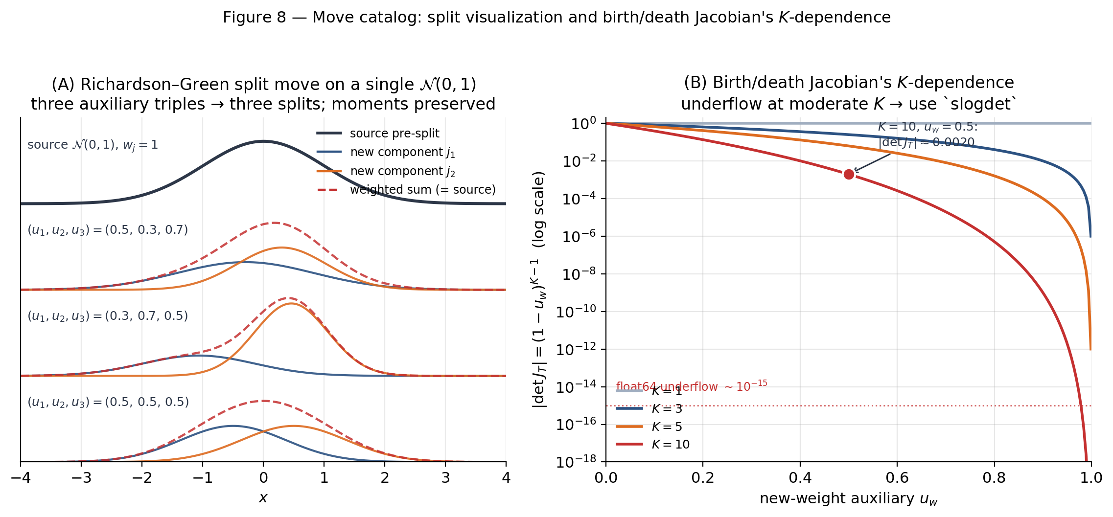
Drag $(u_1, u_2, u_3)$ to see how the auxiliaries control width imbalance ($u_1$), mean separation ($u_2$), and variance allocation ($u_3$). The right panel shows why the birth/death Jacobian crosses float64’s rounding-loss horizon (combined with other small terms in the acceptance ratio) at $K \gtrsim 50$.

u₁ = 0.50

u₂ = 0.50

u₃ = 0.50

μ₁=-0.50, μ₂=0.50, σ₁²=0.75, σ₂²=0.75 · log|det J_split|=1.79

K = 10

§9. Worked example A — Linear-regression variable selection (Kuo–Mallick)

§9 runs the topic’s first complete RJ-MCMC chain. The problem — linear-regression variable selection at $p = 8$ — is small enough that every posterior model probability can be computed exactly by enumerating all $2^8 = 256$ subset-models, so we have a gold-standard reference to validate the chain against.

§9 discharges sparse-bayesian-priors §12.6’s forward-pointer to RJ-MCMC as the discrete-spike-and-slab workhorse, and establishes the validation pattern — “RJ-MCMC vs closed-form gold standard” — that §10’s mixture-order demo relies on by extension.

9.1 The model — Gaussian likelihood, $g$-prior, Scott–Berger model prior

Likelihood. $y_i = \mathbf{x}_i^\top \boldsymbol{\beta} + \varepsilon_i$, $\varepsilon_i \overset{\text{iid}}{\sim} \mathcal{N}(0, \sigma^2)$, with $\boldsymbol{\beta} \in \mathbb{R}^p$. Design matrix $X \in \mathbb{R}^{n \times p}$ treated as fixed (and centered).

Inclusion indicators. $\boldsymbol{\gamma} \in \{0, 1\}^p$: $\gamma_j = 1$ iff covariate $j$ is included. Active set $S = \{j : \gamma_j = 1\}$ with cardinality $|S| = \sum_j \gamma_j$.

$g$-prior on active coefficients.

$$\boldsymbol{\beta}_S \mid S, \sigma^2, g \;\sim\; \mathcal{N}\!\left(\mathbf{0}, \; g\, \sigma^2\, (X_S^\top X_S)^{-1}\right),$$

with $g = n$ (unit-information). $\sigma^2$ is given a flat prior on log scale and marginalized analytically.

Scott–Berger model prior. $p(\boldsymbol{\gamma}) \propto \binom{p}{|\boldsymbol{\gamma}|}^{-1} \cdot \frac{1}{p + 1}$, making model size uniform on $\{0, \ldots, p\}$.

Target. $p(\boldsymbol{\gamma}, \boldsymbol{\beta}_S \mid \mathcal{D}) \propto p(\mathcal{D} \mid \boldsymbol{\beta}_S, \boldsymbol{\gamma})\, p(\boldsymbol{\beta}_S \mid \boldsymbol{\gamma})\, p(\boldsymbol{\gamma})$.

9.2 The add/drop move — single Gaussian auxiliary, Jacobian $\equiv 1$

At each iteration: pick a covariate $j \in \{1, \ldots, p\}$ uniformly and propose to flip $\gamma_j$.

Add move ($\gamma_j = 0 \to \gamma_j = 1$). Draw $u \sim \mathcal{N}(0, \sigma_u^2)$. Bijection $T_m(\boldsymbol{\beta}_S, u) = (\boldsymbol{\beta}_S \text{ with } u \text{ inserted at position } j)$ — identity bijection (permutation). $|\det J_{T_m}| = 1$ exactly.

Drop move. Deterministic: $u = \beta_j$ (the dropped coefficient).

The master acceptance ratio. With $|\det J_{T_m}| = 1$ and $j_{\text{add}} = j_{\text{drop}} = 1/p$, Theorem 3’s master ratio reduces to

$$A_{\text{add}} \;=\; \frac{p(\mathcal{D} \mid \boldsymbol{\beta}_{S \cup \{j\}}, S \cup \{j\}) \, p(\boldsymbol{\beta}_{S \cup \{j\}} \mid S \cup \{j\}) \, p(S \cup \{j\})}{p(\mathcal{D} \mid \boldsymbol{\beta}_S, S) \, p(\boldsymbol{\beta}_S \mid S) \, p(S) \cdot \mathcal{N}(u; 0, \sigma_u^2)}.$$

9.3 The closed-form marginal likelihood and the marginalization shortcut

Under the conjugate $g$-prior, $\boldsymbol{\beta}_S$ can be analytically integrated out. The marginal likelihood is the Liang et al. 2008 eq. (5):

$$\log p(\mathcal{D} \mid S) \;=\; \frac{n - |S| - 1}{2} \log(1 + g) \;-\; \frac{n - 1}{2} \log\!\left(1 + g(1 - R_S^2)\right) \;+\; \text{const},$$

with $R_S^2$ the OLS coefficient of determination of $y$ on $X_S$. The constant cancels in posterior model probability ratios.

The marginalization shortcut. Because $\boldsymbol{\beta}_S$ can be integrated out, the chain doesn’t have to sample it explicitly. The trans-dim machinery reduces to a Metropolis–Hastings chain on $\boldsymbol{\gamma}$ alone with

$$A_{\text{add}}(S \to S \cup \{j\}) \;=\; \frac{p(\mathcal{D} \mid S \cup \{j\})\, p(S \cup \{j\})}{p(\mathcal{D} \mid S)\, p(S)}.$$

Conceptually the chain is RJ-MCMC; implementationally it’s MH on $\boldsymbol{\gamma}$ with one-bit-flip proposals. Approach 1 (sample $(\boldsymbol{\gamma}, \boldsymbol{\beta}_S)$ jointly) and approach 2 (sample $\boldsymbol{\gamma}$ alone with the marginal likelihood) produce identical $\boldsymbol{\gamma}$-marginal posteriors at the same MC sample size. We use approach 2 in §9’s code for efficiency.

9.4 Numerical results — posterior inclusion probabilities and top-model recovery

Setup. $n = 80$, $p = 8$. True coefficients $\boldsymbol{\beta}^\star = (2.5, 0, -1.8, 0, 0, 1.5, 0, 0)$ — three active covariates at indices $\{0, 2, 5\}$. Noise $\sigma = 0.5$. Hyperparameters: $g = n = 80$, Scott–Berger prior.

Enumeration baseline. All 256 subset-models enumerated. Posterior inclusion probabilities $\pi_j$ for each $j$ and model-size posterior computed exactly.

RJ-MCMC chain. 5000 iterations, burn 1000. The log-marginal-likelihood for each visited $\boldsymbol{\gamma}$ is cached in a dictionary keyed by the indicator-vector bitstring.

Results. The chain recovers the enumeration posterior to a maximum inclusion-probability deviation of $0.0255$ (covariate 7 — a noise covariate). All three true-active covariates have $\pi_0 = \pi_2 = \pi_5 = 1.000$ exactly under both enumeration and the chain. The top model $\{0, 2, 5\}$ carries posterior mass $P = 0.5832$ under enumeration; the chain returns $0.5797$. The top-5 model rankings agree with one transposition between ranks 3 and 4. Chain acceptance rate $0.151$; unique models visited $32/256 = 12.5\%$ — the chain concentrates rapidly on the high-posterior region without exhausting the model space.

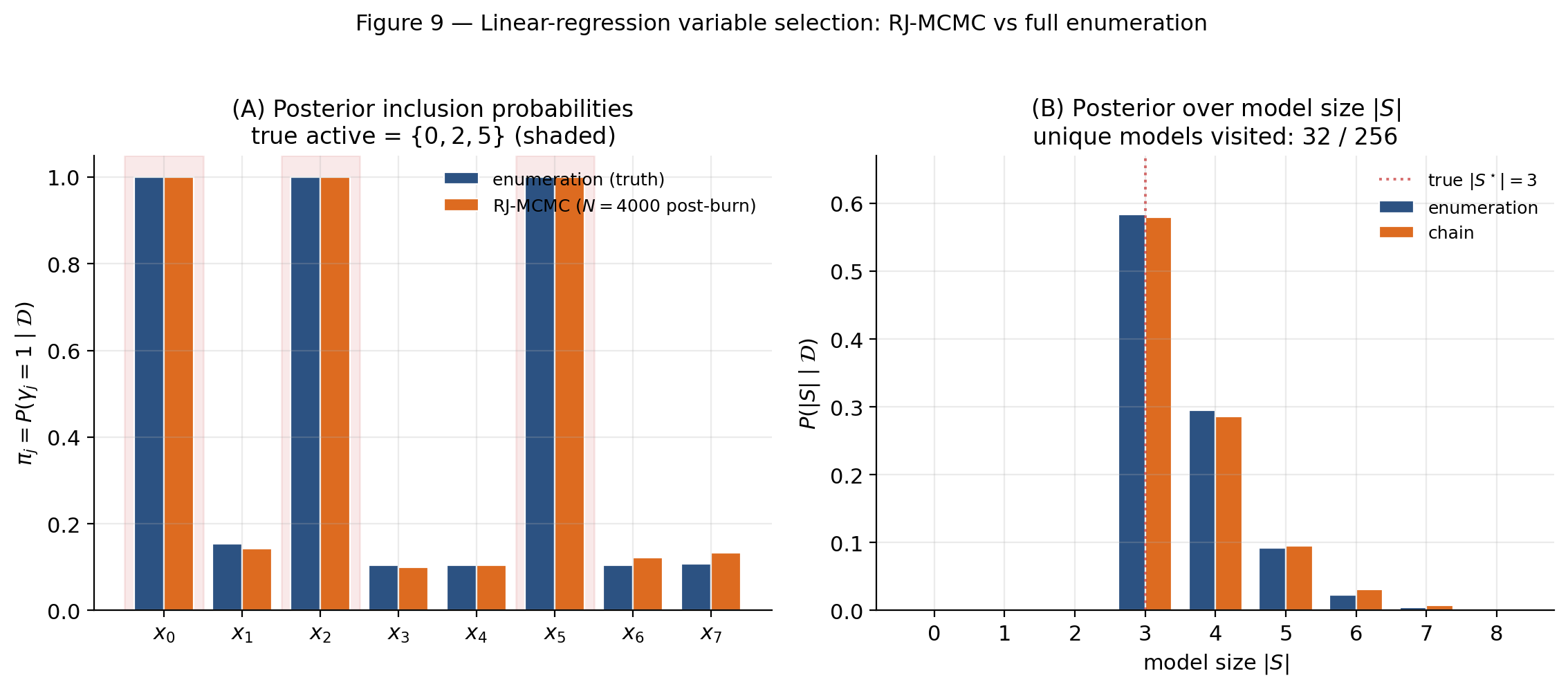
Drop SNR to make the noise covariates indistinguishable from the active ones and watch both posteriors blur together. The chain rerun fires only on slider release; the enumeration baseline always recomputes (256 OLS fits is fast).

SNR (1/σ) = 2.00

g = 80

chain length T = 5000

max |π_enum − π_chain| = 0.0542 · accept 19.7% · unique models visited 32 / 256 = 12.5%

§10. Worked example B — Univariate Gaussian-mixture order estimation (Richardson–Green on Galaxy data)

§10 runs the canonical RJ-MCMC demo: Richardson–Green (1997) on the Galaxy dataset. The chain combines four trans-dim moves (split, merge, birth, death) with a within-model Gibbs sweep, and samples the joint posterior over $(K, \theta_K)$.

Unlike §9, enumeration is not feasible — the parameter space is continuous and the marginal likelihood has no closed form. §9’s validation against enumeration is what makes §10’s posteriors trustworthy by extension.

10.1 The model — finite Gaussian mixture, conjugate priors, $K \sim \mathrm{Uniform}\{1, \ldots, K_{\max}\}$

Data. $n = 82$ Galaxy velocity observations (Roeder 1990), embedded in the notebook’s setup cell.

Mixture model. $y_i \mid \boldsymbol{z}, \boldsymbol{\mu}, \boldsymbol{\sigma}^2 \overset{\text{ind}}{\sim} \mathcal{N}(\mu_{z_i}, \sigma^2_{z_i})$, $z_i \mid \boldsymbol{w} \overset{\text{iid}}{\sim} \mathrm{Categorical}(\boldsymbol{w})$.

Parameter priors. $\mu_j \overset{\text{iid}}{\sim} \mathcal{N}(\xi, \tau^2)$, $\sigma_j^2 \overset{\text{iid}}{\sim} \mathrm{InvGamma}(\alpha_\sigma, \beta_\sigma)$, $\boldsymbol{w} \sim \mathrm{Dirichlet}(\alpha_w, \ldots, \alpha_w)$.

Hyperparameters (data-driven, Richardson–Green style). $\xi = \bar{y}$, $\tau^2 = R^2/16$ where $R = y_{\max} - y_{\min}$, $\alpha_\sigma = 2$, $\beta_\sigma = s_y^2 / 4$, $\alpha_w = 1$. On the Galaxy data: $\xi = 20.83$, $\tau^2 = 39.40$, $\beta_\sigma = 5.153$.

Model prior on $K$. Uniform on $\{1, \ldots, K_{\max}\}$ with $K_{\max} = 6$.

10.2 The split move — Richardson–Green’s bijection, applied component-wise

From §8.2, the split move’s bijection and Jacobian are fully characterized. The closed-form Jacobian:

$$|\det J_{T_{\text{split}}}| \;=\; \frac{w_j \, |\mu_{j_2} - \mu_{j_1}| \, \sigma_{j_1}^2 \, \sigma_{j_2}^2}{\sigma_j^2 \, u_2 (1 - u_2^2) \, u_3 (1 - u_3)}.$$

The merge move picks an adjacent pair in the mean-sorted ordering and applies $T_{\text{split}}^{-1}$ deterministically.

The acceptance ratio for split. With uniform random-scan move-type prior:

$$\log A_{\text{split}} \;=\; \log \pi(K+1, \theta_{K+1}) - \log \pi(K, \theta_K) - \log q(u_1) - \log q(u_2) + \log |\det J_{T_{\text{split}}}|.$$

The Richardson–Green Jacobian is computed in log space directly from the formula.

10.3 The Jacobian determinant in practice — log-space arithmetic and precision guards

The Richardson–Green Jacobian has potential numerical pitfalls: vanishing denominator at $u_2 \to 0$ or $u_2 \to 1$; vanishing $\sigma_{j_1}^2$ or $\sigma_{j_2}^2$ at extreme weight splits. Beta$(2, 2)$ makes these limits exponentially rare. The closed-form $\log |\det J|$ is a sum of elementary logarithms — no matrix needed.

10.4 Birth/death moves and the random-scan catalog

Birth/death is the second trans-dim move pair (§8.1). After the Beta$(1, K)$ / Jacobian cancellation:

$$\log A_{\text{birth}} \;=\; \log \pi(K+1, \theta_{K+1}) - \log \pi(K, \theta_K) - \log q(\mu_{K+1}) - \log q(\sigma^2_{K+1}) - \log K - \log (K+1).$$

Why two trans-dim move catalogs? Split/merge moves $K$ by reshaping an existing component (good at fine-tuning when components are reasonably balanced); birth/death moves $K$ by adding/removing an independent component (good at adding genuinely new components). Together they explore the model space from different directions.

Random-scan catalog. At each iteration, draw uniformly from $\{\text{split}, \text{merge}, \text{birth}, \text{death}, \text{Gibbs}\}$ — five moves with prior $1/5$ each. Invalid moves (split or birth at $K = K_{\max}$; merge or death at $K = 1$) automatically rejected.

10.5 Numerical results on the Galaxy data — posterior over $K$, posterior predictive density

Setup. $n = 82$ Galaxy velocity observations. Hyperparameters as in §10.1. $K_{\max} = 6$. Initial state $K = 2$.

Chain. 5000 iterations, burn 1000.

Posterior over $K$.

$K$	$P(K \mid \mathcal{D})$
3	0.374
4	0.335
5	0.222
6	0.070

Posterior mean $\mathbb{E}[K \mid \mathcal{D}] = 3.99$. The posterior mode lands at $K = 3$, matching Richardson–Green (1997) §6’s reported result; significant mass on $K \in \{4, 5\}$ reflects the data’s ambiguity between three sharp components and four blurry ones.

Per-move acceptance rates. Split $0.118$, merge $0.108$, birth $0.082$, death $0.091$, Gibbs $1.000$ (always accepted). All four trans-dim move rates sit in the “Goldilocks zone” of $5\%$–$50\%$ that §11.4 discusses. Between-$K$ jump rate $8.0\%$.

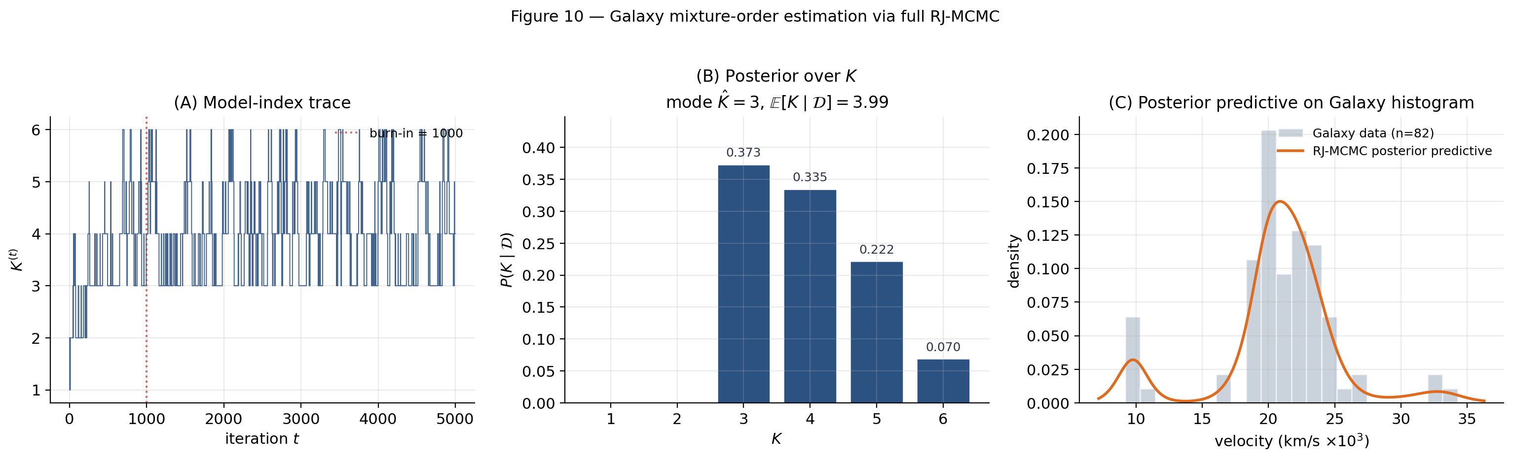
Raise $K_{\max}$ to see whether the posterior chain visits the new high-$K$ models, and widen $\tau^2$ to weaken the prior on component means. The chain rerun fires on slider release.

K_max = 6

τ² scale = 1.00

chain length T = 5000

E[K|D] = 4.17 · mode K = 4 · between-K jump rate 8.6% · trans-dim accept 10.9% · split 13.0%, merge 10.5%, birth 8.4%, death 11.5%

K-trace

P(K | D)

posterior predictive density

§11. Diagnostics for trans-dimensional chains

§11 covers what to look at after the chain has run. Standard MCMC diagnostics ($\hat{R}$, ESS, autocorrelation, trace plots) presume a fixed-dimensional parameter space and a single chain trajectory through it; trans-dim chains break both assumptions.

11.1 Within-model vs across-model diagnostics — the natural decomposition

A trans-dim chain has two sources of variability. The model-index sub-chain $\{K^{(t)}\}$ visits each $K$ with limiting frequency $p(K \mid \mathcal{D})$. The within-model sub-chains $\{\theta_K^{(t)} : K^{(t)} = K\}$, one per model, explore $\Theta_K$ with limiting distribution $p(\theta_K \mid K, \mathcal{D})$.

Standard MCMC diagnostics apply to each within-model sub-chain restricted to the iterations where the chain is in that model. The model-index sub-chain is genuinely new — a discrete-valued time series whose convergence requires diagnostics specifically designed for discrete-state Markov chains.

For Galaxy at $K_{\max} = 6$: one model-index sub-chain on $\{1, \ldots, 6\}$; up to six within-model sub-chains on $(3K - 1)$-dim parameter spaces.

11.2 Convergence of $p(M_k \mid \mathcal{D})$ — running fractions and the multinomial CLT band

Three tools diagnose the convergence of $\widehat{p}(M_k \mid \mathcal{D}) = \frac{1}{N - N_{\text{burn}}} \sum_t \mathbb{1}[K^{(t)} = k]$.

Tool 1: Model-index trace plot. $K^{(t)}$ vs $t$. The chain should hop between $K$ values stationarily — no long monotonic trends.

Tool 2: Running fraction plot. $\widehat{p}_t(K = k)$ vs $t$. At convergence, the curves stabilize near $p_k$.

Tool 3: Multinomial CLT confidence band. $\sigma_t(k) = \sqrt{p_k (1 - p_k) / (t - N_{\text{burn}})}$. A $\pm 2 \sigma_t(k)$ band gives expected fluctuations around the limit. Inflated by $\sqrt{\tau_{\text{iat}}}$ under autocorrelation.

For the §10 Galaxy chain at $t = 4000$ post-burn samples:

$K$	$\widehat{p}_t$	$\pm 2 \sigma_t$
3	0.374	$\pm 0.015$
4	0.335	$\pm 0.015$
5	0.222	$\pm 0.013$
6	0.070	$\pm 0.008$

Between-$K$ jump rate. Fraction of iterations with $K^{(t+1)} \neq K^{(t)}$. Target: $5$–$20\%$ for well-mixing trans-dim chains. The Galaxy chain hits $8.0\%$.

11.3 Within-model ESS — using only the iterations the chain spent in model $k$

Extract the sub-series $\theta_K^{(t_1)}, \ldots, \theta_K^{(t_{M_K})}$ where $\{t_i\} = \{t : K^{(t)} = K\}$, then compute ESS on this sub-series using standard fixed-dim formulas.

Caveats.

• Re-entry effects. When the chain leaves and re-enters $\Theta_K$, the within-$K$ sub-series is interrupted; after re-entry, $\theta_K^{(t_i)}$ may not be drawn from the within-$K$ stationary distribution.
• Snapshot-irregularity caveat. The §10 snapshots are saved every 4th post-burn iteration unconditionally; the filtered within-$K$ subseries is therefore irregularly spaced in iteration time. The IAT $\times$ SNAPSHOT_THIN conversion in §11’s code assumes uniform spacing within-$K$, which is only approximate. Bias is typically $<20\%$ for chains with between-$K$ jump rate $<20\%$ per iteration (the Galaxy chain’s regime).
• Label switching. To compute ESS of a per-component parameter, identify components by sorting (e.g., $\mu_{(1)} < \mu_{(2)} < \cdots$).

For the §10 Galaxy chain at the dominant $K = 3$: $382$ snapshots out of 1000 total; integrated autocorrelation time $\tau_{\text{iat}} \approx 6.6$ iterations; within-model ESS for the smallest-mean component $\approx 233$ — enough for crude summaries.

11.4 Between-model jump acceptance rates — the dimension-changing-move-specific diagnostic

Per-move acceptance rates flag specific tuning problems:

• $< 5\%$: auxiliary proposals too informative; tighten.
• $5$–$50\%$: well-tuned.
• $> 60\%$: auxiliary proposals too conservative; broaden.

For the §10 chain, observed rates: split $0.118$, merge $0.108$, birth $0.082$, death $0.091$ — all four trans-dim moves sit in the Goldilocks zone. The Gibbs move accepts at $1.000$ by construction (closed-form conjugate updates).

The asymmetry between birth/death rates would be expected if the chain prefers reshaping (split/merge) over independent additions (birth/death); on the Galaxy data the rates are similar, which is consistent with the data supporting multiple genuinely different mixture configurations.

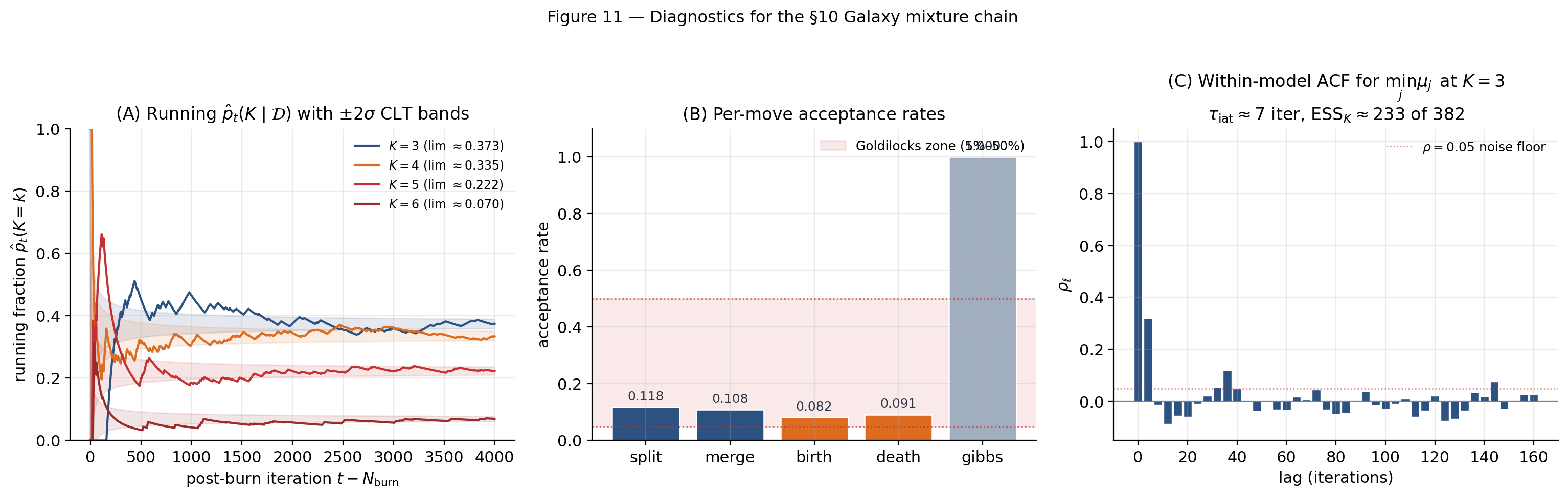
Extend the chain length to watch the running-fraction bands narrow as $1/\sqrt{t}$, the per-move bars stabilize, and the within-$K$ ACF tighten.

chain T = 5000

K_max = 6

running P̂_t(K | D) ± 2σ CLT

per-move acceptance rates

within-K ACF — smallest mean at dominant K

§12. Computational notes

§12 is the implementation-discipline section. It captures the engineering decisions that make §§9–10’s chains run inside the 60-second total budget and keep the on-site implementations responsive.

12.1 Buffer hoisting and the variable-length state vector

Trans-dimensional chains have a variable-length state vector: $\boldsymbol{\mu}, \boldsymbol{\sigma}^2, \boldsymbol{w}$ have length $K^{(t)}$, which changes between iterations. The naive implementation calls np.concatenate, np.append, or list-to-array conversions inside the inner loop — each allocates a fresh array. At 5000 iterations, this adds $20$–$50\%$ to total runtime.

The hoisting fix. Pre-allocate one fixed-size buffer per state component at the maximum dimension $K_{\max}$, plus an integer K_cur tracking the active prefix:

mu_buf = np.empty(K_MAX, dtype=np.float64)
s2_buf = np.empty(K_MAX, dtype=np.float64)
w_buf  = np.empty(K_MAX, dtype=np.float64)
K_cur  = 2

Move functions perform in-place writes on the active prefix.

For §9 (variable selection): no hoisting needed — $\boldsymbol{\gamma}$ is fixed-length, $\boldsymbol{\beta}_S$ is marginalized.

For §10 (Galaxy mixture): the notebook code uses np.concatenate in the move functions for clarity; the on-site live-implementation rewrite hoists into pre-allocated buffers. Notebook prioritizes pedagogical clarity; production prioritizes performance. Same RNG seed produces identical chain output either way.

12.2 slogdet over det — the rounding-loss case

The Jacobian determinant appears in every trans-dim acceptance ratio. For nontrivial bijections at moderate dimension, evaluating $|\det J_{T_m}|$ via det and then taking $\log$ is numerically unsafe — long before the determinant itself underflows to zero, rounding error in the product accumulates and the final log is wrong by several digits.

Precision trajectory for the birth/death Jacobian $(1 - u_w)^{K-1}$ at $u_w = 0.5$ (float64 machine epsilon $\varepsilon \approx 2.2 \times 10^{-16}$; smallest normal $\approx 2.2 \times 10^{-308}$):

$K$	$\|\det J_T\|$	Status
1	$1.0$	safe
10	$1.95 \times 10^{-3}$	safe
30	$1.86 \times 10^{-9}$	representable; precision becoming lossy when multiplied
50	$1.78 \times 10^{-15}$	within ~$10\varepsilon$ — det-then-log accumulates several digits of error
60	$1.73 \times 10^{-18}$	still representable as a double, but products with other small acceptance-ratio terms round to 0

True float64 underflow on this particular Jacobian only happens at $K \gtrsim 1080$ — well past any practically interesting setting. The numerical hazard at $K \approx 50$–$60$ is rounding loss, not underflow per se; the slogdet idiom (or summing elementary logs directly, §8.2) sidesteps both. The Richardson–Green split Jacobian has the same scaling problem at extreme weight splits.

The slogdet idiom. numpy.linalg.slogdet(J) returns $(\text{sign}, \log |\det|)$ directly:

sign_J, log_abs_det_J = np.linalg.slogdet(J_matrix)

log_abs_det_J is well-defined for any $|\det J|$ in float64’s exponent range.

For closed-form Jacobians (§8, §10), we sum elementary logarithms directly — never construct the matrix. The slogdet idiom is for cases where the Jacobian has no closed form.

The rule. Never call numpy.linalg.det in the acceptance-ratio hot path.

12.3 Log-space acceptance-ratio composition

Every component of the master acceptance ratio is computed in log space and summed:

$$\log A_m \;=\; \log \pi(k', \theta_{k'}) - \log \pi(k, \theta_k) + \log j_{\bar{m}} - \log j_m + \log q_{\bar{m}}(u') - \log q_m(u) + \log |\det J_{T_m}|.$$

The acceptance criterion in log space:

if np.log(rng.uniform()) < log_alpha:
    # accept

This is preferable to if rng.uniform() < np.exp(log_alpha) because np.exp overflows for $\log A_m \gg 0$.

For logsumexp operations (mixture-likelihood and model-evidence normalizer): use scipy.special.logsumexp for numerical stability.

The rule. Every density evaluation that feeds into the acceptance ratio returns a log-density. np.exp is called at most once per iteration (at the comparison against log U).

12.4 The outer sampling loop is serial — vectorize the inner linear algebra only

MCMC is intrinsically serial in the iteration dimension. The chain cannot be vectorized across iterations.

Can vectorize: per-iteration linear algebra (proposal densities, log-likelihood, Jacobian, responsibility matrix). The §10 mixture likelihood uses a single broadcast (y[:, None] - mu[None, :]).

Cannot vectorize: outer iteration loop, move-type selection, acceptance decision, state update.

Multi-chain parallelism. Run $K_{\text{chains}}$ independent chains in parallel via multiprocessing.Pool or joblib.Parallel. Each chain still serial; embarrassingly parallel across chains.

§13. Connections and limits

§13 closes the topic with five subsections placing RJ-MCMC in the formalML landscape and the broader Bayesian-computation ecosystem.

13.1 RJ-MCMC closes the specialized-sampler cluster

The T5 Bayesian Computation track has a four-topic specialized-sampler cluster:

• stochastic-gradient-mcmc (SGLD / SGHMC) — noise-injected gradient updates for big-data targets.
• riemann-manifold-hmc (RMHMC) — position-dependent Fisher information mass matrix for pathological fixed-dim targets.
• sequential-monte-carlo (SMC) — particle filters for sequential targets; annealed SMC samplers for evidence estimation.
• reversible-jump-mcmc (this topic) — dimension-changing moves for sampling over a union of model spaces.

RJ-MCMC’s distinctive feature: it’s the only sampler in the cluster that genuinely changes dimension between iterations. After this topic, the specialized-sampler cluster is structurally complete.

13.2 RJ-MCMC vs. variational Bayes for model selection — the bias–variance trade-off

Variational Bayes for Model Selection (coming soon) and RJ-MCMC answer the same question — what is the posterior over models? — with different methods.

VBMS — deterministic, biased. Fit a variational approximation $q_k(\theta_k) \in \mathcal{Q}$ to each candidate posterior, compute the evidence lower bound $\mathrm{ELBO}(q_k, M_k) \leq \log p(\mathcal{D} \mid M_k)$, use ELBO as the model-comparison score.

Properties:

• Biased. By Jensen’s inequality, $\mathrm{ELBO} \leq \log p(\mathcal{D} \mid M_k)$, with the inequality saturated only when $q_k$ matches the true posterior exactly. The gap $\mathrm{ELBO} - \log p(\mathcal{D} \mid M_k) = -\mathrm{KL}(q_k \| p(\theta_k \mid \mathcal{D}, M_k)) \leq 0$, so the bias is downward — ELBO systematically under-estimates the log-evidence by the variational KL gap.
• Fast. One variational optimization per model.
• Limited variational family. The bias depends on the expressiveness of $\mathcal{Q}$.

RJ-MCMC — stochastic, unbiased. Sample directly from $p(K, \theta_K \mid \mathcal{D})$; time-fraction estimator for posterior model probabilities.

Properties:

• Unbiased asymptotically. Under standard MCMC regularity.
• MC error. $\sqrt{p_k (1 - p_k) / N_{\text{eff}}}$.
• Tuning cost. Auxiliary-variable proposals and move-catalog rates need to be tuned per problem.

The practitioner’s choice. Use VBMS for fast scoping; use RJ-MCMC when exact posterior probabilities matter. Often complementary.

13.3 RJ-MCMC vs. SMC samplers

SMC samplers — per-model evidence, then aggregate. Run a separate SMC sampler for each $M_k$; combine via Bayes’ rule. See sequential-monte-carlo §8 for the unbiased log-evidence guarantee.

RJ-MCMC — joint trans-dim sampling. Single chain on the union space; time-fraction estimator.

When SMC wins: small $K$ (2–8 models), per-model evidence is the primary goal, models categorically different.

When RJ-MCMC wins: large $K$ ($\geq 10$ models, $2^p$ for variable selection at $p \geq 5$), models share structure (lattice or dimension stair), joint posterior over (model, parameters) is the goal.

Hybrid workflows use SMC for short-listing and RJ-MCMC for refinement.

13.4 Parametric only — Bayesian nonparametrics is a separate machine

RJ-MCMC’s state space is a countable union of finite-dimensional parameter spaces. Bayesian nonparametric models — DPM, infinite HMMs, IBP, GP, Beta process — have state spaces of unbounded dimension; their samplers exploit the prior process’s special structure (stick-breaking, marginal Pólya urn) and are not RJ-MCMC.

The line: if $K$ has a finite upper bound, use RJ-MCMC. If $K$ is unbounded and the prior process is what defines the model, use a Bayesian nonparametric sampler (Neal 2000’s Algorithm 8 is the canonical reference for Dirichlet process mixtures).

13.5 Tooling notes

PyMC. pm.Mixture handles fixed-$K$ mixtures via marginalization. PyMC does not directly support trans-dim sampling. Standard workflow for model selection: separate per-$K$ models plus pm.sample_smc.

NIMBLE. Supports explicit RJ-MCMC via nimbleMCMC. Recommended starting point for new RJ workflows.

BayesX. Older R package for structured additive regression with RJ-MCMC variable selection. Implements the Lang–Brezger (2004) Bayesian P-spline framework for selecting linear vs nonlinear covariates within a generalized additive model.

Stan. Does not support trans-dim sampling — fundamentally fixed-dim HMC. For variable selection in Stan, marginalize or run per-$K$ + WAIC/LOO.

JAGS / OpenBUGS. Historical RJ-MCMC support via plugin packages, no longer maintained for this feature.

Carlin–Chib product-space samplers. RJ-MCMC subsumes them. Still in some textbooks for pedagogical accessibility; not recommended in new code.

Recommendation. NIMBLE for explicit RJ; PyMC + per-$K$ SMC for marginalized mixtures; custom NumPy/JAX for educational purposes.

13.6 Further reading

The references below are listed in full in the bibliography; we annotate the key entry points here.

The foundational triad. Green (1995) is the original construction; Richardson & Green (1997) is the canonical mixture-order worked example; Hastie & Green (2012) is the modern review with consolidated notation. Start with these three for the historical and methodological arc.

Proposal-construction recipes. Brooks, Giudici & Roberts (2003) give centering and second-order matching techniques for high-acceptance trans-dim moves — the standard reference when the canonical move catalog underperforms.

Variable selection specifics. Kuo & Mallick (1998) for the indicator-variable formulation; Liang et al. (2008) for the hyper-$g$ marginal-likelihood; Scott & Berger (2010) for the multiplicity-correction model prior; O’Hara & Sillanpää (2009) for a comprehensive review of competing approaches.

Handbook and textbook. Brooks, Gelman, Jones & Meng (2011) is the canonical Handbook of Markov Chain Monte Carlo; the Green & Hastie chapter therein is the textbook entry point for RJ-MCMC. Gelman et al. (2013), Bayesian Data Analysis 3rd ed., is the standard graduate textbook with Chapter 11 covering model comparison.