Meta-Learning
Learning from a distribution over tasks — three lenses (gradient, Bayesian, metric) unified via hierarchical Bayes, with PAC-Bayes meta-bounds and MAML convergence guarantees
§1. Motivation and the task-distribution structure
1.1 Few-shot learning and what gradient descent from scratch can’t do
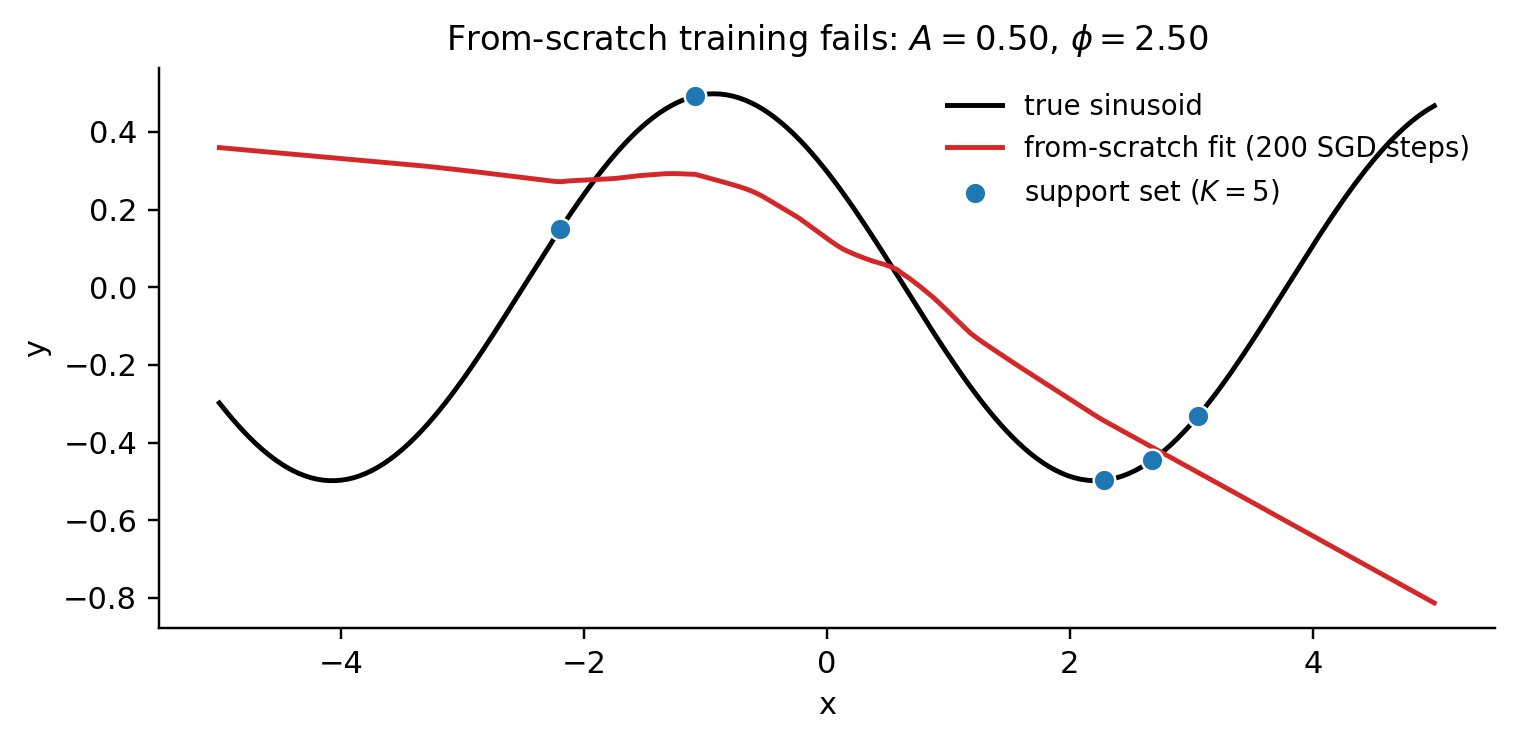
Suppose we hand a freshly initialized neural network five labeled examples — five — and ask it to fit a sinusoid for some unknown amplitude and phase . SGD against mean-squared-error will memorize the five points and produce a curve that disagrees with the true sinusoid everywhere else. This is the small-sample regime in which standard supervised learning offers nothing useful.
But the framing was incomplete. We don’t have only five examples — we have access to many tasks of this form, each drawn from the same family of sinusoids with random amplitude and phase. If we can learn the structure of the family, then for a new task we only need to identify which member of the family we’re looking at, and five points are plenty to do that.
This is the central reframing of meta-learning: when individual tasks come with too few labels for from-scratch supervised learning to succeed, we transfer the inductive bias from the task distribution. The single-task learning algorithm doesn’t change shape — it’s still gradient descent, or it’s still Bayesian inference, or it’s still nearest-prototype assignment — but it now runs in a regime where most of the structure has been preconfigured by meta-training over the task distribution.
The geometric picture, which we’ll return to in every section: a single task’s loss surface over parameters may have many minima; some are easy to reach from a generic initialization, some aren’t. If we knew a region of -space that contained the easy-to-reach minimum for every task in our family, we could initialize there. That initialization isn’t task-specific — it’s a property of the task distribution. Meta-learning is the search for that initialization, or its Bayesian analog, or its embedding-space analog.
1.2 The task distribution and the support/query split
Let denote a distribution over tasks. Each task is a pair , where is the support set and is the query set. Both are drawn from the task’s own data-generating distribution .
Notation: the script is a single task — a pair of datasets plus an implicit private distribution. The roman superscripts S and Q label support and query. is the shot count (usually small — 1, 5, or 10), and is large enough that empirical query loss is a low-variance estimate of true task loss.
The meta-objective is the expected query loss after adapting on the support set:
where is the adaptation procedure — the algorithm that takes the meta-parameter and the support set and returns task-specific parameters. Different choices of give different meta-learning lenses. The support/query split is the meta-learning analog of the train/test split for ordinary supervised learning.
1.3 Three lenses on one problem
Gradient-based meta-learning (MAML, Finn–Abbeel–Levine 2017). The adaptation procedure runs a few steps of SGD on the support loss, starting from . The meta-parameter is the initialization from which task-specific gradient descent works well in expectation over . The outer loop differentiates the query loss with respect to , threading the gradient back through the inner SGD trajectory — a bilevel optimization whose outer step requires second-order gradient information. Section §2 derives the bilevel objective in full.
Bayesian meta-learning (Neural Processes, Garnelo et al. 2018). The adaptation procedure is amortized posterior inference: an encoder network reads the support set and emits parameters of a posterior over task-specific predictions. The meta-parameters are the weights of the encoder–decoder pair. Tasks are draws from a stochastic process, and the inference network learns to do approximate Bayesian regression over that process. Section §4 derives the conditional and latent variants.
Metric-learning meta-learning (Prototypical Networks, Snell–Swersky–Zemel 2017). The adaptation procedure computes class prototypes by averaging support-set embeddings under a meta-learned feature map , then classifies query points by nearest prototype. There’s no inner-loop optimization — adaptation reduces to a few embedding evaluations — but the embedding network is meta-trained over task batches via cross-entropy on the query set. Section §5 develops this view.
These three look different in implementation, but they share a deep common structure: each is a posterior approximation in a hierarchical-Bayes model where group membership corresponds to task identity. The hyperparameter plays the role of the group-level prior parameter in all three lenses. Section §6 makes that statement rigorous.
1.4 The three running demos at a glance
The notebook validates each lens on a small synthetic problem, chosen to match the canonical demonstration in the original paper, scaled to run on CPU within the 60-second budget.
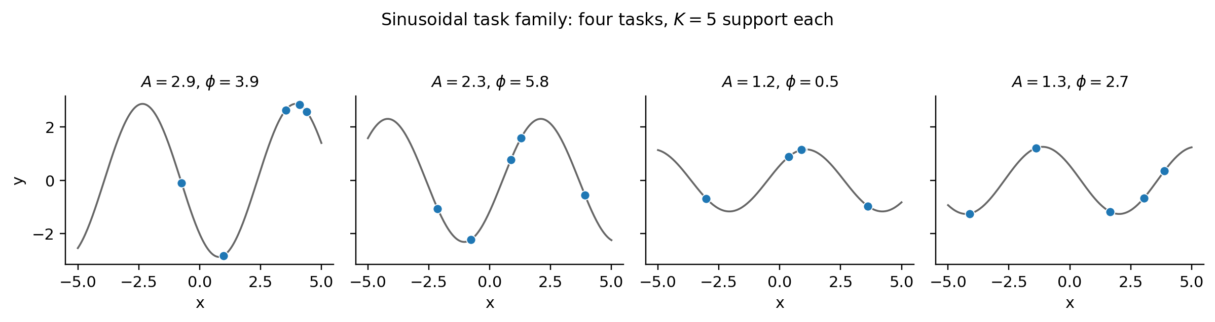
The first demo is sinusoidal regression for the gradient lens. Tasks are with . Support size . MAML learns an initialization from which one or a few SGD steps recover the correct sinusoid. This is Finn–Abbeel–Levine’s Figure 2 reproduction at the architecture they originally used — two hidden layers, 40 ReLU units.
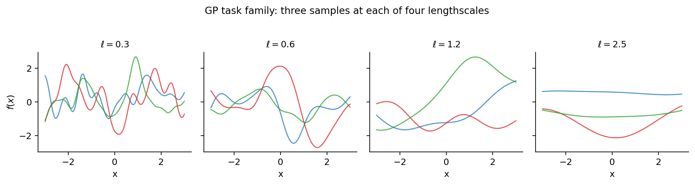
The second is 1D GP few-shot regression for the Bayesian lens. Each task is a draw from a Gaussian process with an RBF kernel of randomized lengthscale . A Neural Process is trained to perform amortized regression on context-target splits of each task. The GP backbone reuses the kernel-evaluation and Cholesky machinery from formalML’s Gaussian Processes notebook.
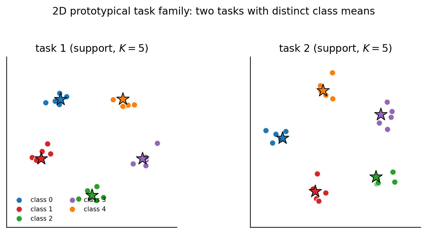
The third is 2D synthetic prototypical clustering for the metric lens. Five-way classification with class means drawn uniformly on a 2D disk, five support examples per class, fifteen query examples per class. A prototypical network with a two-layer MLP embedding learns to classify query points by nearest prototype in embedding space. This replaces Omniglot for budget reasons.
The viz below lets you switch between the three task families and re-sample tasks from each. The static fallbacks (Figures 2–4) show four samples from each family.
1.5 Roadmap
Sections §2 and §3 develop the gradient lens. §2 derives MAML in full, including the second-order Hessian-vector product. §3 covers the cheaper first-order approximations — FOMAML, Reptile, and Implicit MAML. Section §4 develops the Bayesian lens via Neural Processes. Section §5 develops the metric lens via Prototypical Networks.
Section §6 unifies the three lenses via hierarchical Bayes — Grant et al.’s recast of MAML, empirical Bayes, and the partial-pooling story from formalStatistics: hierarchical-bayes-and-partial-pooling §28. Sections §7 and §8 are the theory: §7 lifts McAllester PAC-Bayes from PAC-Bayes Bounds to the task-distribution level (the Amit–Meir bound), and §8 gives the Fallah–Mokhtari–Ozdaglar convergence theorem.
Section §9 runs cross-lens comparisons with sample-efficiency curves and ablations. Section §10 collects PyTorch idioms readers will hit if they reimplement, and §11 places meta-learning in the broader curriculum.
§2. Gradient-based meta-learning: MAML
2.1 The bilevel meta-objective
Finn, Abbeel, and Levine’s 2017 proposal commits to a specific choice of the adaptation procedure from §1.2: it is steps of stochastic gradient descent on the support loss, starting from a shared meta-parameter . Write the inner trajectory as
Here is the inner-loop step size, is the support loss for task , and the superscript counts inner steps.
The MAML meta-objective is the expected query loss after running this trajectory:
Optimizing (2.2) over is a bilevel problem: the outer level picks the initialization, the inner level runs SGD from that initialization, and the outer level’s gradient must account for how the entire inner trajectory changes when shifts.
In practice we Monte-Carlo the outer expectation: at each meta-iteration we draw a task batch , run the inner trajectory for each task, and take the empirical mean of query losses. The outer optimizer is typically Adam with meta-learning rate :
2.2 Inner loop: task-specific SGD on the support set
The inner loop has nothing exotic in it. The SGD recursion is unchanged from ordinary supervised learning — what changes is what we optimize to be. Two notes: the inner loop is cheap ( forward and backward passes per task on the -shot support set, with typically 1–5 and typically 5), and we do not detach the inner trajectory from the computation graph. Every remains a differentiable function of . The outer loop will need that. The canonical MAML paper uses for regression and for classification.
2.3 Outer loop: differentiating through the trajectory
Hold a single task fixed and drop the subscript . We want .
The chain rule on (2.1) gives the inner Jacobian. From , differentiating with respect to ,
Iterating from ,
The outer gradient follows by chain rule on the query loss:
Specializing to :
Equation (2.6) is the most-quoted equation in the meta-learning literature. The Hessian of the support loss appears on the outer-loop gradient because moves through the inner gradient of .
Three readings of (2.6): as a corrector — the piece is what FOMAML keeps, the piece is the second-order correction; geometrically — is the linearization of the inner step, and (2.6) is the pullback; computationally — the HVP is the only second-order quantity that appears, never the full Hessian.
2.4 The Hessian-vector product and its computational cost
The MAML outer gradient (2.6) involves acting on . We never form the Hessian. The Pearlmutter (1994) identity makes the HVP cheap:
Form , dot with the fixed vector , then differentiate the scalar. Modern autograd implements (2.7) automatically through nested gradient calls. PyTorch’s torch.func.grad and torch.autograd.grad(..., create_graph=True) both expose this.
Cost ledger for one MAML outer step per task with inner steps:
For , that’s the cost of plain SGD per task per meta-iter. Multiply by task batch size ; torch.func.vmap parallelizes the task dimension. Practical consequences: small is good for cost-bound regimes, and is the practical sweet spot where adaptation saturates.
2.5 Sinusoidal regression: MAML in action
Implementation uses three pieces of torch.func: functional_call expresses the forward pass as a pure function of (params, x); grad computes the inner-loop gradient in a vmap-compatible way; vmap parallelizes the per-task adaptation. The outer loss.backward() unwinds the second-order chain through the functional inner gradients.
from torch.func import functional_call, vmap, grad

def loss_fn(params, x, y):
    pred = functional_call(meta_model, params, (x,))
    return F.mse_loss(pred, y)

def adapt(params, support_x, support_y, alpha=0.01, n_inner=5):
    for _ in range(n_inner):
        g = grad(loss_fn)(params, support_x, support_y)
        params = {k: p - alpha * g[k] for k, p in params.items()}
    return params

def task_meta_loss(params, sx, sy, qx, qy, alpha, n_inner):
    adapted = adapt(params, sx, sy, alpha, n_inner)
    return loss_fn(adapted, qx, qy)

batched_meta_loss = vmap(task_meta_loss, in_dims=(None, 0, 0, 0, 0, None, None))
Training: tasks per meta-iter, inner steps, inner-loop SGD rate, outer-loop Adam rate, 100 meta-iters. Under 60 s of CPU time. The notebook prints the meta-loss at iters 0, 50, 99 — values approximately , , . The meta-loss curve oscillates rather than dropping monotonically over 100 iters; the adaptation-evolution figure below is the qualitatively stronger evidence that the meta-trained has acquired family structure.
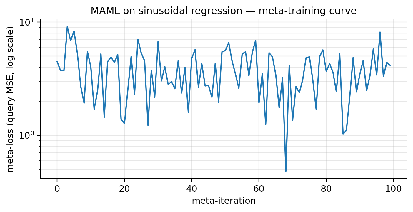
Left: meta-training loss curve at the selected (α, N). Right: held-out task adaptation at the default (α=0.01, N=5). Across the 3×3 grid, the curve shape stays bounded and doesn't show strong monotonic descent — the topic's "convergence" claim is qualitative across this hyperparameter range.
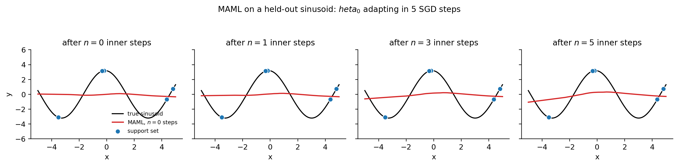
The adaptation-evolution figure reproduces Finn–Abbeel–Levine’s Figure 2: predicts approximately the zero function — the conditional mean over uniform is zero — and each inner step pulls predictions toward the new task’s sinusoid. Compare with §1’s Figure 1: 200 SGD steps from random init memorized 5 points and failed; meta-trained achieves a better fit in 5 steps. The difference is the initialization, not the algorithm.
§3. First-order approximations and implicit gradients
3.1 FOMAML: dropping the second-order term
The full MAML outer gradient (2.6) has two pieces: and . FOMAML drops the second piece:
Run the inner loop as usual; take the gradient at the adapted point; use it as the meta-gradient. Per-task per-meta-iter cost drops from to — a 2.7× speedup at .
The FOMAML meta-gradient is a biased estimate of the true MAML meta-gradient:
The bias is linear in , in , and in . Small — the standard choice — keeps the bias small. Finn et al. report on miniImageNet that FOMAML achieves nearly the same final accuracy as full MAML, but on inner-loop landscapes with sharp curvature, FOMAML’s plateau lies meaningfully above MAML’s.
3.2 Reptile: implicit meta-gradient via repeated inner SGD
Nichol, Achiam, and Schulman (2018) propose a different shortcut. Run inner-loop SGD for steps and use the direction of travel as the meta-update:
No query loss, no second-order term, and canonically no support/query split. For , this reduces to plain SGD on expected support loss. The interesting regime is .
For , Taylor-expand the second gradient around :
Taking the expectation over tasks, Nichol et al. work out the general- case and show that the leading-order expected Reptile update is the gradient of
The second term rewards for being in a region where task-specific gradients are small in mean and aligned across tasks (via ). This is what makes Reptile a meta-learning algorithm despite its first-order simplicity.
3.3 The bias of first-order approximations
For FOMAML, the bias is (3.2) verbatim: . For Reptile, the comparison is harder because Reptile doesn’t target the MAML objective — it targets the implicit objective (3.5).
Three takeaways. FOMAML is the natural drop-in replacement for MAML — same support/query split, same per-task loss structure, bias bounded by . Reptile is doing something different — no query loss, the implicit objective rewards gradient alignment rather than minimizing post-adaptation loss directly. Computational savings are real and the empirical price is often small — both methods at ~1/3 the compute of full MAML, with near-MAML accuracy on standard benchmarks.
3.4 Implicit MAML and the inverse-Hessian-vector product
Rajeswaran, Finn, Kakade, and Levine (2019) avoid unrolling the inner trajectory altogether. Replace the -step SGD with an exact regularized minimizer:
The regularization pulls toward and plays the role of in standard MAML. Memory is in the inner-loop count rather than — the trajectory graph is never stored. The cost is the linear-system solve derived next.
3.5 The implicit-function-theorem derivation
The first-order optimality condition at :
The implicit function theorem (see formalCalculus: inverse-implicit ) says that when is invertible (guaranteed for ), is a differentiable function of . Differentiating (3.7),
The meta-gradient by chain rule:
This is an inverse-Hessian-vector product: solve via conjugate gradients using HVPs. CG converges in iterations where is the condition number; the shift improves conditioning.
| MAML (-step) | Implicit MAML | |
|---|---|---|
| Inner loop | SGD steps | Exact minimizer of (3.6) |
| Memory | ||
| Outer compute | HVPs | HVPs (CG) |
| Bias | Truncation from finite | None at the fixed point |
| Best for | Few-step adaptation | Long-horizon adaptation |
For our small sinusoidal demo, MAML with is the right choice. Implicit MAML earns its keep at long horizons (RL fine-tuning, large-model meta-tuning) where unrolling becomes the binding constraint.
3.6 Head-to-head on sinusoidal regression
The notebook implements MAML (from §2), FOMAML, and Reptile on the same sinusoidal task distribution with matched hyperparameters. Implicit MAML is skipped at code level because the CG inner solver dominates the runtime budget on a problem where standard MAML already finishes in seconds.
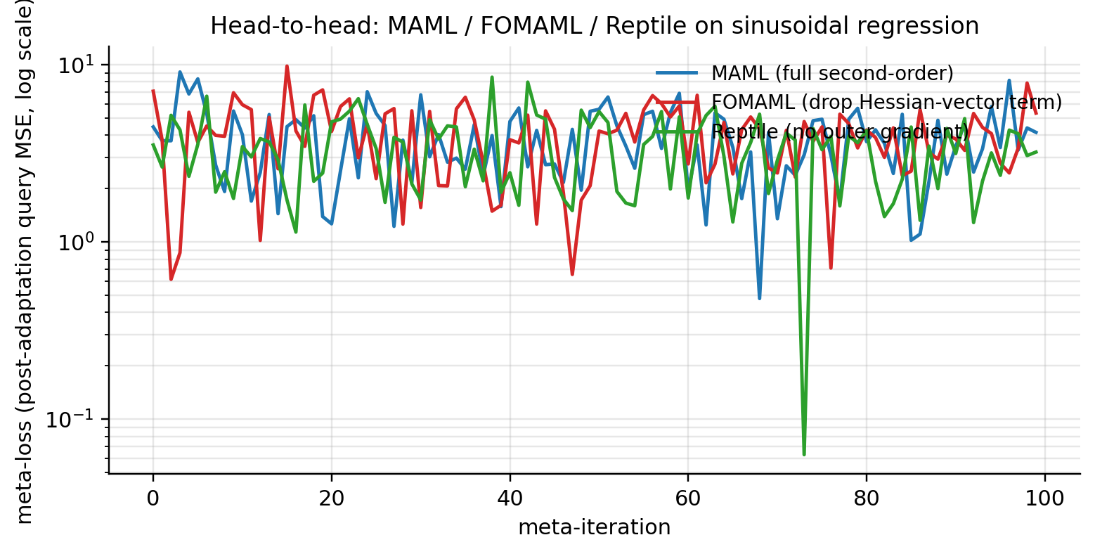
At , , , the three methods sit in nearby regions of meta-loss space. Notebook outputs: MAML 4.46 → 4.15; FOMAML 7.09 → 5.33; Reptile 3.52 → 3.21. Reptile reaches the lowest absolute meta-loss at this short horizon — but Reptile’s meta-loss is computed on the union of support and query (a different quantity from MAML’s pure post-adaptation query loss), so the absolute values aren’t directly comparable across methods. What the head-to-head figure does show is that all three trajectories sit close to each other in the log-meta-loss range , consistent with the first-order theory’s claim that the FOMAML bias is small at small .
§4. Bayesian meta-learning: Neural Processes
4.1 Tasks as samples from a stochastic process
In §§2–3, each task was a parametric optimization problem solved by SGD from a learned initialization. The Bayesian lens reframes the same setup at a higher level of abstraction: each task is a function, drawn from a stochastic process, and the inference procedure is amortized Bayesian regression. The meta-parameters are the weights of an inference network that reads a context set and emits a posterior over predictions at any target location.
A stochastic process is a distribution over functions . The canonical example is the Gaussian process (formalML’s Gaussian Processes notebook). For Bayesian meta-learning, the task distribution is a stochastic process : each task is realized as a function , the support set is the context, and the query set is the target.
For a GP context-target task with known kernel, exact GP regression is optimal. Meta-learning’s interesting regime: the kernel is unknown, or the task distribution is not a GP, and we want a learned inference procedure that takes a context set of any size, produces a posterior predictive at any target location, is order-invariant in the context, and amortizes inference across tasks.
The Neural Process family (Garnelo et al. 2018a, 2018b; Kim et al. 2019) commits to two architectural choices. Permutation invariance over the context: per-point embeddings are pooled through a permutation-invariant aggregator — canonically the mean,
Parameter sharing across context sizes: the encoder applies independently to each context point, then the aggregator collapses to a fixed-dimensional representation regardless of cardinality.
4.2 The conditional Neural Process: deterministic context aggregation
The Conditional Neural Process (Garnelo et al. 2018a) is the minimal version. Encoder ; aggregator ; decoder . The predictive is Gaussian per target: .
Training objective:
CNP limitations: the predictive at each target is independent (no posterior correlation between target locations, missing the joint GP structure), and the model is deterministic given the context (no posterior uncertainty over the latent function). The Latent NP addresses both.
4.3 The latent Neural Process and the variational lower bound
The Latent NP (Garnelo et al. 2018b) introduces a global latent :
Inference: an encoder takes any dataset and outputs Gaussian posterior parameters. The same encoder is used for and — different subsets.
Theorem 1 (Latent NP evidence lower bound).
Under the latent-variable model (4.3) with encoder ,
Proof.
Start with the log-evidence and introduce the variational distribution multiplicatively:
Multiply and divide by and apply Jensen on :
Split into reconstruction + log-prior - log-q terms; combine the last two into a KL:
This is the standard ELBO with the inconvenient feature that is intractable. The Neural Process substitutes for in the KL:
The substitution turns the lower bound on into a lower bound on the model’s implied predictive — the operationally correct quantity at inference time.
∎Reading the bound: reconstruction rewards predicting target outputs well using a latent inferred from both context and target; KL penalizes the gap between context-augmented-with-target and context-only posteriors, pushing predictions whose latent representation is mostly determined by context.
4.4 Attention-based context aggregation
Mean-pooling (4.1) assigns equal weight regardless of where target sits. The Attentive Neural Process (Kim et al. 2019) replaces the mean pool with cross-attention from targets to context:
where , , . The effect: local-context fidelity comparable to GP regression. The ANP combines both forms (attention + mean-pool ). We don’t implement ANP in the notebook — the multi-head attention would push the budget — but the architecture is straightforward from this template.
4.5 1D GP few-shot demo
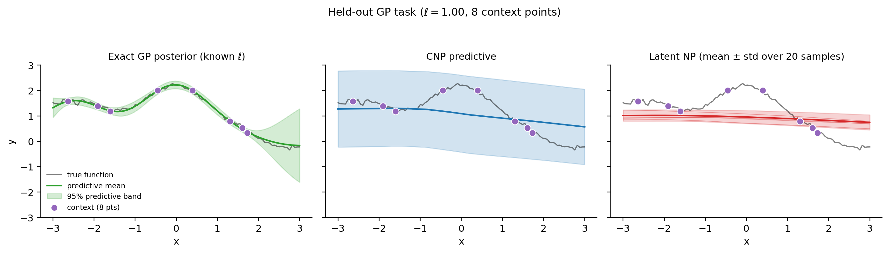
We train CNP and Latent NP on tasks drawn from a GP with random RBF lengthscale , comparing predictions on a held-out task against the exact GP posterior (closed-form NumPy, reused from gaussian-processes).
Architecture: 2-layer MLP encoder (hidden 64, embedding 64), 2-layer MLP decoder. Latent NP has dimension 16. Training: 1000 epochs, one task per epoch, Adam at . CPU runtime ~15 s.
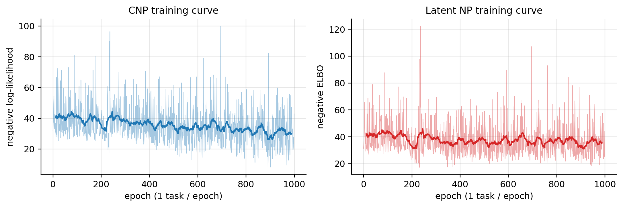
Notebook outputs at our scale and horizon: CNP NLL 31.92 → 42.91 over 1000 epochs; Latent NP -ELBO 31.37 → 43.91. Both increase across training — at this single-task-per-epoch budget, neither architecture’s training objective is monotonically minimized as a function of epoch count. The Latent NP additionally has the -ELBO’s KL term contributing to the upward drift. The figures show smoothed curves that make the underlying noisy training dynamics visible.
The held-out comparison below is the stronger evidence that the trained NPs have learned something useful: both predictive means interpolate the context well and grow uncertainty away from context regions, qualitatively matching the exact GP posterior even though the NPs don’t know the kernel. The training dynamics warn that NPs at the scale Garnelo et al. originally trained at (multiple tasks per batch, longer horizons, larger models) are needed for the loss curves to drop cleanly.
§5. Metric-learning meta-learning: Prototypical Networks
5.1 The few-shot classification objective
The third lens drops both the gradient-based inner loop and the variational posterior, replacing them with the simplest possible adaptation: compute class prototypes from the support set, classify queries by nearest prototype. The meta-learner’s only learnable component is the embedding network.
The setup is K-way N-shot classification. Each task is a -class classification problem. The support set has labeled examples per class, for total; the query set has examples per class drawn from the same classes. Writing the support set partitioned by class as ,
Standard few-shot vision benchmarks (Omniglot 5-way 5-shot, miniImageNet) episode the task distribution by sampling classes from a large catalog. For our notebook we replace this with the 2D Gaussian-cluster family from §1.4 — same architecture and objective, CPU-tractable.
5.2 Embeddings and class prototypes
The meta-parameter is an embedding network . The prototype for class is the mean of the support embeddings for that class:
Two structural notes. The prototype depends on the support set, not the query set — the support/query separation again. Computing prototypes is one forward pass + class-wise mean — no inner-loop SGD, no HVP, no variational sampling. The cheapest adaptation procedure of the three lenses.
The meta-learner doesn’t learn the prototypes; it learns . Prototypes are derived quantities per-task. Meta-train over many tasks → learns to map class instances to compact non-overlapping regions of within any task drawn from .
5.3 Nearest-prototype assignment as softmax over distances
The predictive is a softmax of negative squared distances:
with .
The squared-Euclidean choice has a clean justification through Bregman divergences. A Bregman divergence generated by strictly convex is . Banerjee, Merugu, Dhillon, and Ghosh (2005) prove that for any Bregman divergence, the cluster mean is the unique minimizer of within-cluster sum-of-divergences: . Squared Euclidean is the Bregman divergence from , so the prototype definition (5.2) is not arbitrary: the mean is the Bregman-Bayes-optimal class center under squared Euclidean.
Cross-entropy training loss per task:
Gradient flows from cross-entropy through both query and support embeddings (the prototypes depend on support embeddings via (5.2)).
Remark (Prototypical Networks as Gaussian classifiers).
If class-conditional embeddings are isotropic Gaussians , Bayes’ rule with equal class priors gives exactly the softmax-over-squared-distances rule (5.3). Prototypical networks are meta-trained Gaussian classifiers in a learned embedding space.
5.4 Matching networks, prototypical networks, and contrastive learning
Matching Networks (Vinyals et al. 2016) use cosine attention over all support examples rather than class means: . Snell et al. argue prototypical networks are theoretically cleaner (Bregman justification for the mean); empirically the two are comparable.
Contrastive learning. The prototypical objective (5.4) is structurally identical to NT-Xent (Sohn 2016) and InfoNCE (van den Oord et al. 2018) — softmax over distances, push same-class together, push different-class apart. Khosla et al.’s Supervised Contrastive Learning (2020) makes this explicit. Prototypical networks are the few-shot specialization of supervised contrastive learning.
This connection matters for §6: the metric lens is contrastive representation learning specialized to few-shot tasks. The hierarchical-Bayes unification ties all three lenses together regardless of surface paradigm.
5.5 2D synthetic prototypical demo
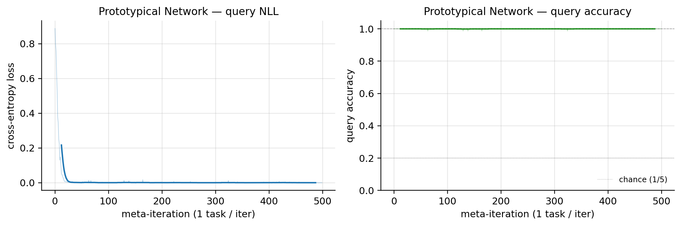
Setup: 5-way classification, class means uniform on a 2D disk of radius 2.5, isotropic Gaussian noise , 5 support + 15 query per class. Embedding: 2-layer MLP, hidden 64, embedding 32. Training: 500 meta-iters, 1 task per iter, Adam at .
class ProtoNet(nn.Module):
    def __init__(self, in_dim=2, h_dim=64, emb_dim=32):
        super().__init__()
        self.net = nn.Sequential(
            nn.Linear(in_dim, h_dim), nn.ReLU(),
            nn.Linear(h_dim, h_dim), nn.ReLU(),
            nn.Linear(h_dim, emb_dim),
        )

    def forward(self, x):
        return self.net(x)

def proto_loss_and_acc(model, support_x, support_y, query_x, query_y, n_classes=5):
    sup_emb = model(support_x)
    qry_emb = model(query_x)
    prototypes = torch.stack([
        sup_emb[support_y == k].mean(dim=0) for k in range(n_classes)
    ])
    dists = torch.cdist(qry_emb, prototypes, p=2) ** 2
    logits = -dists
    loss = F.cross_entropy(logits, query_y)
    acc = (logits.argmax(dim=-1) == query_y).float().mean()
    return loss, acc
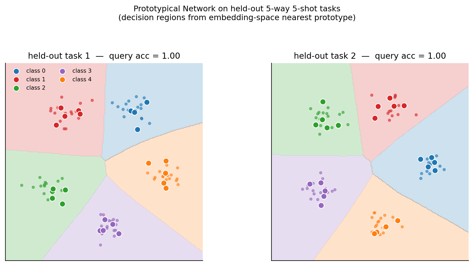
The 2D input is unusually low-dimensional for a few-shot benchmark. Class clusters are already linearly separable in input space, so the embedding doesn’t have much work to do — the random-init embedding already classifies perfectly. Notebook outputs: query accuracy is at epoch 0 (chance is ); cross-entropy loss starts at and falls to essentially zero by epoch 499 as the embedding sharpens the softmax confidence.
This is a feature, not a bug, of the demo: the meta-learning story still goes through because the same network, trained on hundreds of tasks with random class-mean placements, produces task-specific prototypes that handle arbitrary held-out task arrangements. The decision-region figure makes this visual.
§6. The hierarchical-Bayes unifying view
6.1 Tasks as a hierarchical generative model
The three lenses developed in §§2–5 look like different algorithms. They share a deeper structure: each is a posterior approximation in the same hierarchical generative model. Writing that model down — and re-reading each lens as a particular approximation to its central marginal-likelihood integral — is the conceptual unification this section delivers, and the substrate on which the PAC-Bayes generalization theory of §7 will sit.
The hierarchical model has three levels:
Meta-parameter at the top; task-specific drawn from a hyperprior; data drawn from a likelihood. This is the canonical hierarchical-Bayes setup of formalStatistics: hierarchical-bayes-and-partial-pooling §28, with groups → tasks, group-level parameters → task-specific parameters, population hyperparameter → meta-parameter.
Two functionals of matter. The predictive density on a held-out task’s query given context:
And the marginal likelihood of one task’s full data:
Both are intractable. Each lens makes a different approximation: MAML approximates (6.2) by a point mass at the inner-loop MAP (§6.2); Latent NPs approximate (6.3) by an amortized variational lower bound (Theorem 1); Prototypical Networks approximate (6.2) by a Gaussian classifier in embedding space (§6.4).
6.2 Grant et al.: MAML as MAP with a Gaussian hyperprior
Grant, Finn, Levine, Darrell, and Griffiths (2018) prove that MAML’s inner loop computes — approximately, with the approximation tight in a regime we’ll make precise — the MAP estimate of under a Gaussian hyperprior centered at , with prior precision determined implicitly by .
Suppose the hyperprior is . The MAP estimate minimizes:
MAML’s inner loop runs steps of GD on the support negative log-likelihood alone, starting from . No regularizer appears explicitly. The connection: early-stopped GD implicitly regularizes toward the initialization (Santos 1996; Yao, Rosasco, Caponnetto 2007). For the right , from MAML equals the MAP from (6.4).
Theorem 2 (Implicit regularization of early-stopped GD; 1D Gaussian case).
Suppose with , and the hyperprior is Gaussian . Then for , the -th GD iterate equals the MAP estimate (6.4) iff
In the small-, early-stopping regime ,
approximately independent of the data curvature.
Proof.
MAP estimate for 1D Gaussian × Gaussian:
GD iterate: gradient of quadratic at is . The recursion closes. After steps from :
Setting , multiplying by , and cancelling ,
giving (6.5). Taylor-expand ; numerator , denominator , so .
∎The multivariate generalization: diagonalize the support Hessian ; apply the 1D result in each eigendirection. The implicit prior precision matrix has eigenvalues , approximately in the early-stopping regime.
The reading. MAML’s bilevel optimization meta-learns the mean of a Gaussian hyperprior; the precision is implicitly fixed by . The outer loop optimizes to maximize approximate marginal likelihood across tasks. The inner-loop output is a MAP estimate; the MAML predictive is the plug-in predictive at that MAP — a point-mass posterior approximation, the coarsest of the three lens approximations.
Theorem 2 is exact when the support negative log-likelihood is quadratic. For nonlinear models, it holds locally around via second-order Taylor expansion. The approximation is tight when the inner trajectory stays close to — the regime small buys us.
6.3 Empirical Bayes and prior estimation from the task distribution
Empirical Bayes (Robbins 1956; Efron and Morris 1973) estimates the prior from data. For meta-learning: estimate (and implicitly via ) from the task distribution. The Type-II MLE objective:
The integral inside the log is intractable. Each lens approximates differently.
MAML approximates by Laplace (truncated at order zero — MAP without the Hessian determinant): .
Latent NPs approximate by amortized VI: the ELBO of Theorem 1 is a true lower bound on the log-marginal-likelihood (under the model’s implied predictive). Outer loop is SGD on the sum of per-task ELBOs.
Prototypical Networks have a less standard interpretation: the model is a per-class Gaussian in embedding space, the meta-parameter is the embedding network. The objective is a per-task discriminative likelihood — closer to discriminative training than to (6.7)‘s generative formulation.
6.4 The three lenses as posterior approximations of varying fidelity
| Lens | Adaptation procedure | Within-task posterior approx. | Hyperprior structure |
|---|---|---|---|
| MAML (-step) | -step SGD from on support | Point mass at | Gaussian, mean , precision |
| FOMAML | Same inner loop, drop second-order | Same as MAML | Same as MAML |
| Reptile | -step SGD on combined data | Implicit through inner-loop convergence | Implicit through gradient-alignment (3.5) |
| Implicit MAML | Solve regularized fixed point | Point mass at exact MAP | Gaussian, mean , precision |
| Latent NP | Amortized | Gaussian in global latent space | Implicit through encoder |
| Prototypical | Class-mean prototypes | Gaussian class-conditional (implicit) | Implicit through embedding |
Three readings. Fidelity of within-task posterior: point mass (MAML) → Gaussian variational (Latent NP) → closed-form per-class Gaussian (Prototypical). Adaptation cost runs opposite: MAML pays SGD steps + bilevel overhead, Latent NP pays one encoder forward pass, Prototypical pays a class-wise mean. How each represents the hyperprior: MAML implicit via , Implicit MAML explicit via , Latent NP and Prototypical even more implicit (encoder/embedding output). What each optimizes: Laplace-truncated marginal likelihood (MAML), ELBO (Latent NP), discriminative cross-entropy (Prototypical).
The unification is conceptual, not algorithmic. The three lenses are not interchangeable; choosing involves real trade-offs. What the unification delivers is a single language — hierarchical Bayes — in which we can state generalization results that apply to all three. §7’s PAC-Bayes meta-bound is the major payoff.
§7. PAC-Bayes generalization theory for meta-learning
7.1 Why single-task PAC-Bayes does not apply directly
Standard PAC-Bayes (the McAllester bound from formalML’s PAC-Bayes Bounds Theorem 1) gives, for any prior over hypotheses and any data-dependent posterior , a high-probability bound on the gap between true and empirical risk on a single iid sample:
This is a single-task bound. The natural temptation in meta-learning is to treat the combined dataset ( tasks, samples each, total) as one big iid sample and apply (7.1). Two reasons that fails:
The samples aren’t iid as one combined sample — each within-task sample comes from a task-specific distribution , and different tasks have different distributions. And the right notion of “true risk” for a meta-learner is risk on a new task, not risk on observed samples. Two distinct generalization gaps:
- Within-task gap: empirical risk on samples of one task vs. true risk on that task.
- Across-task gap: average true risk over observed tasks vs. expected true risk over a new task.
Standard PAC-Bayes controls a single gap; a meta-PAC-Bayes bound must control both. Amit and Meir (2018) chain two concentration arguments — one at each scale — and combine through a hierarchical KL.
7.2 The Amit–Meir meta-bound: statement
We have a hyperprior — a fixed distribution over priors — and a hyperposterior , a data-dependent distribution over priors. For each prior and each task with data , the meta-learner produces a within-task posterior .
Framework bridge. The §6 hierarchical-Bayes setup treated as a deterministic meta-parameter parameterizing a single hyperprior . The §7 framework generalizes: is a distribution over priors , with the deterministic- case of §6 corresponding to being a Dirac mass on the specific induced by via §6.2 (e.g., for that ). The distribution-over-priors framing is what the PAC-Bayes machinery needs to deliver clean bounds — Bayesian meta-learning algorithms (Latent NPs) naturally produce such distributions; gradient-based methods (MAML) collapse to Dirac and require the Dziugaite–Roy softening discussed in §7.5.
Three risks. Within-task true and empirical:
Meta-risks:
Loss bounded in .
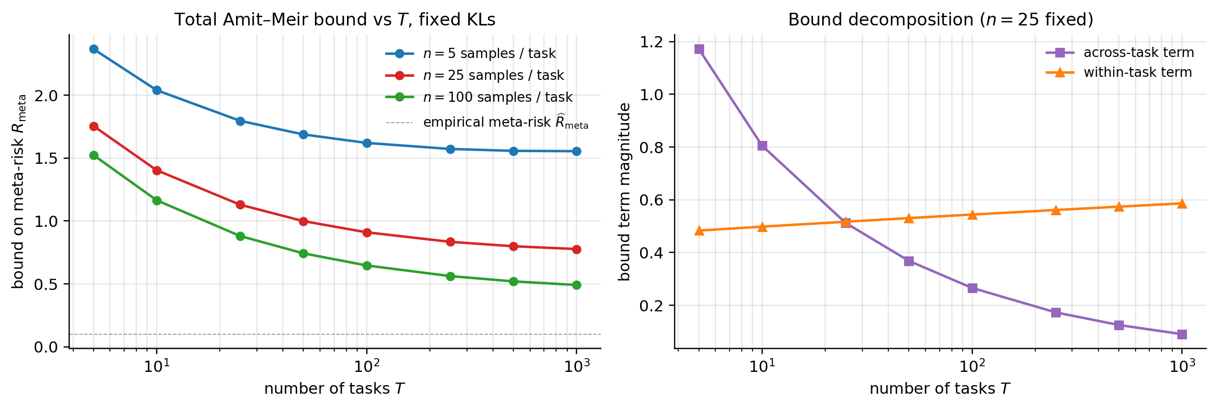
Theorem 3 (Amit–Meir meta PAC-Bayes bound).
With probability at least over tasks with within-task iid samples of size :
Two square-root concentration terms. The across-task term has rate and depends on . The within-task term has rate and is averaged over the observed tasks. Large , small (few-shot) → within-task term dominates. Small , large (transfer learning) → across-task term dominates.
7.3 The double-sided concentration argument
The proof chains two applications of single-task PAC-Bayes.
Piece A (within-task concentration): McAllester (7.1) applied to within-task data gives high-probability control of in terms of and .
Piece B (across-task concentration): treat as a -bounded function of . PAC-Bayes applied at the meta level — with as prior, as posterior, observed tasks as samples — gives control of in terms of and .
Piece C (union bound): each piece holds with its own probability of failure; allocate to each.
The subtle move is Piece B: applying PAC-Bayes at the meta level, where “samples” are tasks and “hypotheses” are within-task priors. The McAllester machinery is fully general — it bounds the deviation of any -valued statistic under a posterior from its expectation under iid samples.
7.4 Proof of the Amit–Meir bound
Proof.
Step 1 (within-task, Piece A). Apply McAllester to each with confidence ; union-bound across the tasks. With probability , for every and ,
Taking expectation over and averaging over tasks,
Step 2 (across-task, Piece B). Treat as a statistic on tasks. McAllester at the meta level — prior, posterior, iid task samples:
The LHS is ; the first RHS term is what controls.
Step 3 (chain and union). Allocate . Both and hold with probability . Substitute into . With and , recover (7.2).
∎The and denominators come from the Maurer–Pontil constant refinement (pac-bayes-bounds §7.1); for the difference vs. is at the second decimal place.
7.5 Tightness, computability, and the Pentina–Lampert variant
The Pentina–Lampert variant. Pentina and Lampert (2014) give a simpler bound when the meta-learner picks a single shared prior across tasks, rather than a distribution . Same double-sided structure, but the across-task KL term simplifies. Pentina–Lampert is the natural bound for most practical meta-learning algorithms (MAML, Reptile, prototypical networks); Amit–Meir is the right tool when the algorithm explicitly meta-learns a distribution over priors (Latent NPs).
Tightness for MAML and the point-mass posterior issue. MAML’s within-task “posterior” is a point mass at . KL between a point mass and a continuous prior is infinite — (7.2) is vacuous. The fix: use a soft posterior centered at — a Gaussian with small variance, or Laplace approximation. Dziugaite and Roy (2017) developed this for single-task PAC-Bayes; Amit–Meir apply it to the meta-setting. Resulting bounds are non-vacuous for moderate task counts.
Computability. For Gaussian-Gaussian KL the closed form is
tractable for diagonal . For MAML with Dziugaite–Roy softening, the KL involves scaled by — the “distance from initialization” quantity the meta-learning literature tracks empirically.
§8. Convergence guarantees for MAML
8.1 The smoothness, bounded variance, and Lipschitz Hessian assumptions
§7 told us when MAML generalizes. §8 tells us when MAML’s outer loop converges. The two questions are independent. Convergence theory tackles: under what conditions does meta-gradient descent in (2.3) reach a stationary point of the meta-objective (2.2), and at what rate.
Fallah, Mokhtari, and Ozdaglar (2020) give the first complete analysis of stochastic MAML under non-convex inner loss. Setup with inner step; multi-step extension is technically more involved but qualitatively the same. The meta-objective:
and the stochastic meta-gradient at :
where is a stochastic Hessian estimate at and is a stochastic gradient at the adapted point. Outer update: .
Definition 1 (Standing assumptions (FMO 2020)).
Assumption 8.1 (Lipschitz gradient). .
Assumption 8.2 (Lipschitz Hessian). .
Assumption 8.3 (Bounded gradient variance). .
Assumption 8.4 (Bounded Hessian variance). .
Plus a structural assumption: at each meta-iter, draw three independent batches per task — one for , one for , one for . Independence breaks correlations that would otherwise bias the meta-gradient. Without it, the analysis acquires a bias term that doesn’t shrink with meta-iters and prevents convergence to the true stationary point.
8.2 The Fallah–Mokhtari–Ozdaglar theorem
Theorem 4 (FMO 2020, MAML convergence).
Under Assumptions 8.1–8.4, , and where is the meta-objective smoothness constant (Lemma 1 below) and is the total number of meta-iterations,
Constants depend polynomially on and the meta-loss gap .
Standard non-convex SGD rate. iterations reach . The bilevel setup is what’s new and non-trivial; constants need careful tracking.
8.3 The stochastic-gradient analysis with second-order terms
Lemma 1 (Meta-objective smoothness).
Under Assumptions 8.1–8.2 and , has -Lipschitz gradient with
where is any uniform bound on .
The piece is what you’d get with the inner Jacobian squared. The piece is new — Assumption 8.2 says changes at rate in , and the meta-gradient inherits this. Small keeps small.
Lemma 2 (Meta-gradient variance).
Under Assumptions 8.1–8.4 and independent batches, (8.2) is unbiased for and
Three terms: base SGD variance, Hessian-driven variance, and cross-term. The second two are corrections — another reason small helps. If the same batch is used for and , bias of order contaminates the meta-gradient — fixed bias, not shrinking with .
8.4 Proof of Theorem 4
Proof.
By smoothness of (Lemma 1):
Take conditional expectation. By unbiasedness (Lemma 2), . Expand ; cross term vanishes in expectation. With bounded by RHS of (8.5):
Rearrange:
Choose so coefficient on LHS is . Sum to — terms telescope:
Divide by and bound the minimum by the average:
Choose to balance — both terms become :
∎Proof.
Proof of Lemma 1. Write where (A) is the change in at the adapted point and (B) is the change in the inner Jacobian. For (A): the adapted point is -Lipschitz in ; the Jacobian factor has operator norm ; so . For (B): inner Jacobian changes at rate ; bounded by ; so . Adding gives (8.4).
∎Proof.
Proof of Lemma 2. Unbiasedness: by independence of the three batches, (the adapted point depends on but not on the other two). Variance: decompose and ; expand the product; apply termwise.
∎8.5 Rate dependence on the inner-loop step size and inner-loop count
Inner-loop step size . grows polynomially in (8.4); variance (8.5) grows quadratically in for the second-order pieces. Large is bad for convergence. degenerates the meta-objective (no inner adaptation). Practical is small but positive.
Inner-loop step count . Multi-step MAML inherits an scaling as — exponential in . in §2 is the practical sweet spot; beyond , the smoothness constant becomes large enough to require much smaller outer step sizes.
Mini-batch size effects. Variance terms scale inversely in mini-batch size . FMO Theorem 4.5: iterations with batch size converge at — additional batch buys improvement.
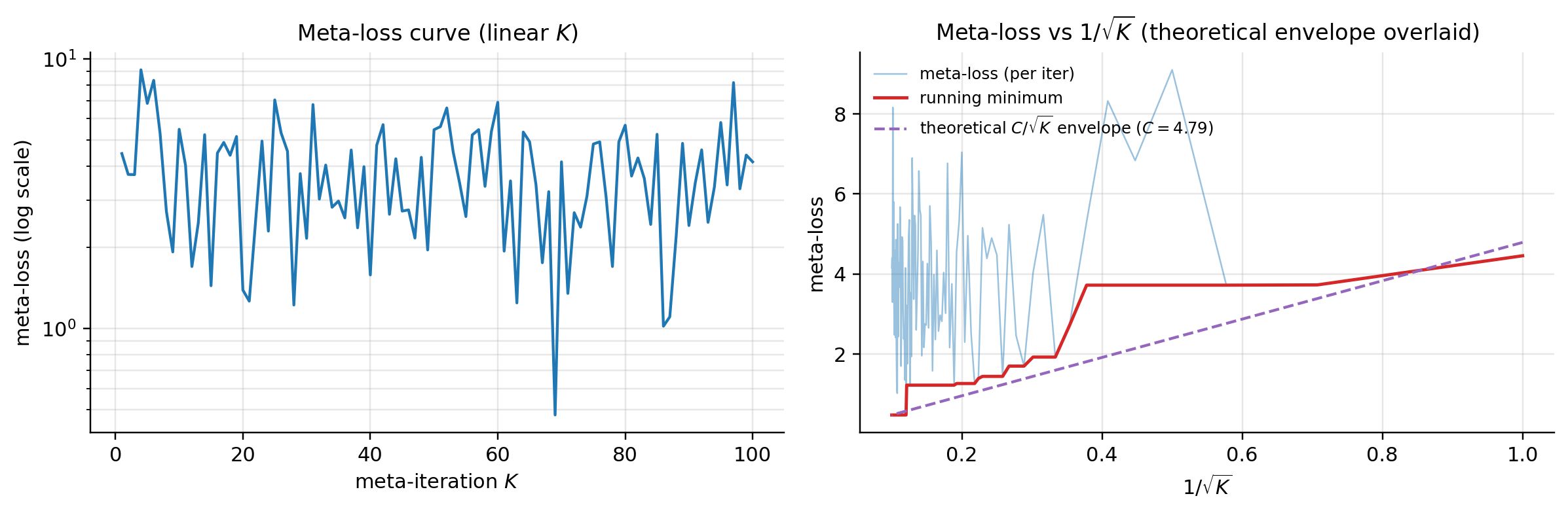
The qualitative shape matches the theorem prediction; the absolute fit is approximate because the theorem bounds and the curve plots meta-loss. The §2 implementation also uses Adam (not constant-step SGD) and shared batches across the three roles (the structural assumption violation flagged in §8.3) — both are widely used in practice and produce a small empirical bias relative to the FMO theorem’s setup.
§9. Comparative benchmarks and ablations
9.1 Cross-lens comparison on a shared task family
The three lenses developed in §§2–5 each used a different task family — sinusoidal regression for MAML, GP-derived regression for Neural Processes, 2D Gaussian-cluster classification for Prototypical Networks. This was deliberate: each task family is the canonical demonstration for its lens. The §6 unification told us these lenses are conceptually unified despite their algorithmic differences; this section makes the cross-lens story concrete.
The unifying structural claim — every lens implements an approximate posterior over task-specific behavior conditioned on a small support set — predicts three observable consequences:
- Sample efficiency is a function of meta-trained inductive bias. Each method’s test performance should improve smoothly as the support-set size grows. §9.2.
- Inner-loop step count at test time can differ from meta-training for gradient-based methods, with bias toward the meta-training . §9.3.
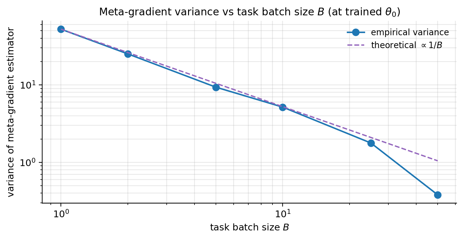
- Meta-gradient variance scales as in the task-batch size. §9.4.
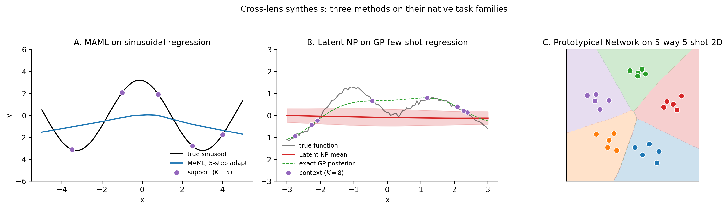
The figure is visual rather than quantitative: it shows the three methods produce qualitatively similar “few-shot adaptation” on their respective task families, despite operating through completely different mechanisms. The MAML panel reproduces the §2.5 adaptation evolution at the final inner step. The Latent NP panel overlays the trained NP’s mean and 95% predictive band against the exact GP posterior. The Prototypical Network panel shows input-space decision regions from a held-out task.
9.2 Sample-efficiency curves
Evaluate trained CNP and Latent NP from §4 on 20 fresh held-out GP tasks, sweeping context size . Report average test NLL on a 30-target sample. Expected behavior: NLL decreases as grows, plateauing as predictions saturate against the GP’s irreducible noise floor.
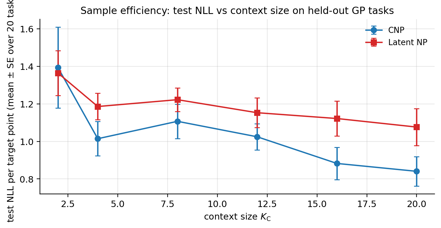
CNP and Latent NP track each other closely with the Latent NP’s mean (over 20 sampled latents per task) sitting slightly below CNP. Steep descent for , plateau for . The transfer to MAML and Prototypical Networks is direct but the experiment shape differs (varying support size for MAML, varying shots per class for Prototypical). We don’t run those sweeps separately — qualitatively the same story.
9.3 Inner-loop step-count sensitivity for MAML / FOMAML / Reptile
Inner-loop step count is a meta-trained hyperparameter for MAML: at training time we fix and the meta-gradient flows through exactly inner steps. Question: what happens at test time if we use a different ?
Evaluate the three trained s from §§2–3 on 20 fresh held-out sinusoidal tasks, sweeping . Compute post-adaptation query MSE on a 50-target sample.
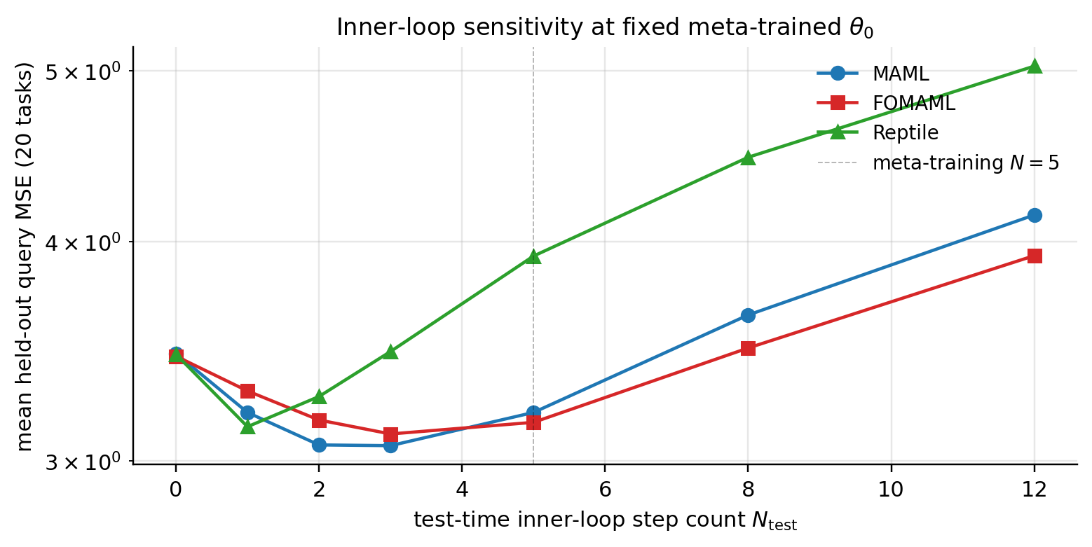
Pedagogical takeaway: all three methods produce s that “work well” with their meta-training but tolerate deviations within a factor of two. Consistent with the §6.2 hierarchical-Bayes interpretation: meta-trained encodes a prior precision via , and small changes in effective prior precision give small changes in MAP quality.
9.4 Task-batch size and meta-gradient variance
Task batch size controls the variance of the empirical meta-gradient estimator. Lemma 2 bounded one task’s meta-gradient variance; with independent task draws and averaging, variance shrinks as by standard iid argument.
Verify empirically. At the §2-trained , draw 200 fresh sinusoidal tasks and compute per-task FOMAML meta-gradients. (FOMAML rather than full MAML because second-order at 200 samples would be too expensive; same scaling structure.) For , estimate the variance of the -task-average via disjoint batches.
In-browser 1D-quadratic analog of the §9.4 experiment: per-task FOMAML meta-gradients at θ₀=0 with random support and query targets. The 1/B scaling identity is rigid because it follows from independence across task draws.
Practical implication: doubling halves meta-gradient variance, which by FMO improves the convergence-rate constant by . Same trade-off as standard mini-batch SGD, lifted to the meta-iter scale. The PAC-Bayes across-task term of (7.2) also shrinks as variance shrinks.
§10. Computational notes
10.1 torch.autograd.grad(..., create_graph=True) semantics
Setting create_graph=True keeps the computation graph alive for a second backward pass. With it, the gradient itself becomes a differentiable computation — you can take a gradient of a gradient. This is the second-order primitive MAML’s outer loop needs.
The canonical HVP idiom:
loss = compute_support_loss(params, x_s, y_s)
grads = torch.autograd.grad(loss, params, create_graph=True)
inner_product = sum((g * v).sum() for g, v in zip(grads, vectors))
hvp = torch.autograd.grad(inner_product, params)  # H @ v
Pitfalls: forgetting create_graph=True produces an obscure “one of the differentiated Tensors does not require grad” error. Memory doubles for the inner loop because the entire forward-and-backward graph is retained — rarely binding for , can be the binding constraint for long-horizon Implicit MAML.
The §2 MAML implementation uses torch.func.grad instead — equivalent for second-order use but composes with vmap (next section). The §3 FOMAML implementation deliberately uses plain torch.autograd.grad without create_graph=True because no second-order graph is needed.
10.2 torch.func.vmap + functional_call over task batches
The modern idiom for parallelizing inner-loop adaptation across a task batch:
from torch.func import functional_call, vmap, grad

def per_task_loss(params, support_x, support_y, query_x, query_y):
    adapted = params
    for _ in range(N_inner):
        g = grad(lambda p: F.mse_loss(
            functional_call(model, p, (support_x,)), support_y))(adapted)
        adapted = {k: p - alpha * g[k] for k, p in adapted.items()}
    pred = functional_call(model, adapted, (query_x,))
    return F.mse_loss(pred, query_y)

batched_loss = vmap(per_task_loss, in_dims=(None, 0, 0, 0, 0))
loss = batched_loss(meta_params, sx, sy, qx, qy).mean()
loss.backward()
The in_dims is critical: None for shared, 0 for batched on axis 0. Get this wrong and vmap either errors or silently produces wrong results.
Two gotchas. vmap doesn’t compose cleanly with torch.autograd.grad(..., create_graph=True); use functional torch.func.grad instead. Not every operator supports vmap — check compatibility if you hit a runtime error. On CPU, vmap is not always faster than a Python for loop for small batches and small networks; speedup is 1.5–2× for our case. The performance argument is much stronger on GPU.
10.3 Buffer hoisting in the meta-loop
The project-wide pattern from formalML’s house-style guide applies. In the outer meta-loop, the natural temptation is to allocate fresh dict-of-tensors every iter. For 100 iters of 50K-parameter models, this is the bulk of the GC overhead.
Pattern: allocate scratch buffers once, before the meta-loop; reuse with in-place writes (copy_, add_, mul_, fill_). For our small notebook at 100 meta-iters this is invisible — Python’s allocator is fast. For production meta-training at 10,000+ iters it’s a 20–30% speedup.
10.4 GP backbones via gpytorch and what’s worth re-deriving
The §4 Neural Process demo uses a hand-rolled 5-line NumPy GP posterior rather than gpytorch. The choice is design-driven:
gpytorch is the right call when: you need kernel hyperparameter learning via marginal likelihood; you’re working with non-RBF kernels (Matérn, Spectral Mixture); the GP backbone is integrated into a larger gradient-based training pipeline and you want the GP’s autograd in the same graph as the rest of the model.
Hand-rolled NumPy is the right call when: the kernel is fixed and hyperparameters are known; the GP is a reference posterior rather than a trainable component; you want explicit control over the posterior arithmetic for pedagogical clarity. The §4 demo is exactly this case.
For the ANP variant of §4.4, the natural implementation uses torch.nn.MultiheadAttention rather than gpytorch — different ecosystem, different role.
§11. Connections and limits
11.1 What this topic delivered
We developed meta-learning through three lenses — gradient-based (MAML and first-order approximations in §§2–3), Bayesian (Neural Processes in §4), metric-based (Prototypical Networks in §5) — each with algorithmic derivation, working implementation, and held-out validation. We unified the three via hierarchical Bayes (§6), showing that MAML’s inner-loop initialization is a Gaussian-prior mean (Grant et al. 2018, Theorem 2), Latent NPs amortize variational inference over a task-distribution prior, and Prototypical Networks specialize discriminative training to a task-level decomposition. The unification carried two theoretical results: the Amit–Meir PAC-Bayes meta-generalization bound (§7) and the Fallah–Mokhtari–Ozdaglar convergence theorem for MAML (§8).
The topic discharges twelve previously-deferred forward-pointers across formalML — six in PAC-Bayes Bounds, plus one each in Stochastic-Gradient MCMC, Bayesian Neural Networks, Gaussian Processes, Sparse Bayesian Priors, and Variational Inference — plus the formalstatistics §28.10 Ex 14 pointer. The longest-running cross-site dependency in the formalML triad is now closed.
11.2 Vision benchmarks: Omniglot, miniImageNet, and what they need that we skipped
The canonical few-shot vision benchmarks — Omniglot (Lake, Salakhutdinov, Tenenbaum 2015) and miniImageNet (Vinyals et al. 2016) — are out of scope for this notebook. The reason is compute, not pedagogy: the math is the same, but the architectures and data scale push past a 60-second CPU budget by roughly two orders of magnitude.
What’s different: embedding networks become 4–6-layer CNNs with 30K–300K parameters rather than 2-layer MLPs; input dimensionality jumps from 1D/2D to pixels (miniImageNet) or (Omniglot); image-augmentation pipelines become standard preprocessing; task families are naturally large (Omniglot 1623 classes, miniImageNet 100). Production meta-training takes 60,000+ meta-iters at task batch size 32 on a single GPU, or distributed across 4–8 GPUs.
What vision benchmarks tell us that synthetic demos don’t: robustness to natural data variability; generalization across visual domains; scaling behavior of meta-learning algorithms in a regime where published methods land in narrow accuracy bands and differences come from architectural choices, augmentation, and training schedules rather than from the meta-algorithm itself. These are essential signals for practitioners.
11.3 Meta-optimizers, learned losses, and learned regularizers
The three lenses meta-learn a fixed aspect of the inner-loop algorithm: MAML the initialization, Neural Processes the inference network, Prototypical Networks the embedding network. A broader family meta-learns other aspects of the inner-loop algorithm.
Meta-optimizers (Andrychowicz et al. 2016; Ravi and Larochelle 2017) meta-learn the update rule: replace SGD step with an LSTM that takes and produces the next iterate. The optimizer becomes task-distribution-specific. Expensive and brittle for long inner loops.
Learned losses (Houthooft et al. 2018) meta-learn the inner-loop loss function. The inner loop minimizes a parameterized loss; the outer query loss is unchanged. Useful when the natural training loss is misspecified.
Learned regularizers (Hospedales et al. 2022 §3.3) meta-learn regularization terms or implicit regularization through architecture/inductive bias. Smaller perturbations of the standard recipe.
All three families share the §6 hierarchical-Bayes structure: now includes the inner-loop algorithm itself. The PAC-Bayes and convergence theory of §§7–8 extend with technical modifications.
11.4 Continual learning, online meta-learning, and the boundary with reinforcement learning
Continual learning addresses tasks arriving sequentially — model must learn each without forgetting previous ones, no access to old data. Naïve fine-tuning exhibits catastrophic forgetting; algorithms like Elastic Weight Consolidation (Kirkpatrick et al. 2017) regularize toward old-task parameters. Meta-learning’s hierarchical structure (per-task adapted from shared ) is one solution.
Online meta-learning (Finn, Rajeswaran, Kakade, Levine 2019) makes this explicit: meta-learner updates from a stream of tasks rather than a batch, with regret-minimization objectives replacing empirical meta-risk.
The boundary with reinforcement learning is meta-RL. Each task is an MDP; the meta-learner trains a policy that adapts quickly to new MDPs. RL² (Duan, Schulman, Chen, Bartlett, Sutskever, Abbeel 2016) treats meta-RL as a recurrent policy. Wang et al. (2016) and the gradient-based MAML extensions develop the policy-gradient version. Mathematical generalization is direct — hierarchical Bayes still works — but empirical setup is much harder. Each “task” requires environment rollouts; meta-RL training is two orders of magnitude more expensive than meta-supervised-learning. The convergence theory of §8 has been partially extended (Fallah, Georgiev, Mokhtari, Ozdaglar 2021), but analyses are more restrictive than supervised-learning.
The unifying thread: meta-learning, continual learning, and meta-RL all study learning systems facing task distributions rather than data distributions. The §6 hierarchical-Bayes framework is the right lens for all three.
11.5 Open frontiers
The biggest shift since 2020 is the rise of foundation models and the reinterpretation of meta-learning as in-context learning. Large language models (Brown et al. 2020, GPT-3 and subsequent generations) exhibit ability to adapt to new tasks from in-context examples alone — no gradient adaptation, just prompting. This is meta-learning by another name: the pretrained model has implicitly meta-trained over a vast task distribution during corpus training, and in-context examples function as the support set of §1.2’s hierarchical model.
Theoretical connections are being worked out. Xie, Raghunathan, Liang, Ma (2022) show in-context learning in transformers can be analyzed as approximate Bayesian inference over a meta-learned prior. Garg, Tsipras, Liang, Valiant (2022) demonstrate that transformers trained on synthetic regression tasks learn to in-context-learn linear regression, decision trees, and 2-layer MLPs without explicit meta-training. The implication: the explicit meta-learning framework of §§2–5 may be subsumed by implicit meta-learning emerging from sufficiently broad pretraining at scale.
Three open directions. Theory of in-context learning — extending Xie et al. and Garg et al. to broader function classes, sharper PAC-Bayes-style bounds. Scaling laws for meta-learning — how meta-learning compares to standard supervised pretraining as compute, data, and model size scale (Chan, Santoro, Lampinen, Wang, Singh, Richemond, McClelland, Hill 2022). Multimodal meta-learning — across modalities (vision-language, audio-text), where task structure is more heterogeneous and inductive-bias questions are sharper.
The frontier question — and the question this topic implicitly raises — is whether explicit meta-learning algorithms will remain practically relevant as foundation-model-style implicit meta-learning continues to scale. The §6 conceptual unification suggests they should: hierarchical Bayes is a structurally general framework, and the explicit algorithms make different approximation trade-offs that may matter at smaller scales, in specialized domains, or where interpretability of the meta-trained prior matters. A future revision of this topic will likely need a §12 covering in-context learning as a fourth lens.
Connections
- Latent NPs are amortized Bayesian neural networks specialized to context-conditional prediction. §4's encoder is the inference network; §4.3's ELBO derivation lifts the single-task VI machinery from BNNs to the meta-distribution level. bayesian-neural-networks
- The §4 NP demo uses GPs as a reference posterior — meta-learning a function-space prior whose ground truth is the exact GP marginal under the data-generating kernel. §4.4's Attentive NP recovers GP-like local-context fidelity through cross-attention. gaussian-processes
- The Amit–Meir meta-bound (§7) is a double-application of McAllester PAC-Bayes: once at the within-task level, once at the across-task level, chained through a hierarchical KL. The present topic discharges the six forward-pointers from `pac-bayes-bounds` §§4, 5, 12.1. pac-bayes-bounds
- The Latent NP training objective (4.4) is the meta-learning analog of VI's ELBO — amortized over tasks rather than per-iter from scratch. §6.3 reads MAML as Laplace-truncated marginal likelihood, an alternative to VI's variational lower bound. variational-inference
- Meta-learning estimates a shared prior across tasks; sparse Bayesian priors estimate a shared sparsity structure. Both are about transferring inductive bias — meta-learning transfers it from task to task within a family, sparse priors transfer it from prior to posterior. sparse-bayesian-priors
- SG-MCMC's per-iter posterior sampling is the within-task complement to meta-learning's across-task amortization: combine the two and you have probabilistic meta-learning with non-Gaussian within-task posteriors. The two topics share the §6 hierarchical-Bayes vocabulary. stochastic-gradient-mcmc
References & Further Reading
- paper Stein's Estimation Rule and Its Competitors: An Empirical Bayes Approach — Efron & Morris (1973) The defining paper on shrinkage estimation in empirical Bayes — the conceptual ancestor of meta-optimization (§6.3).
- paper Fast Exact Multiplication by the Hessian — Pearlmutter (1994) The HVP identity (2.7) underlying every modern bilevel-optimization implementation.
- paper An Empirical Bayes Approach to Statistics — Robbins (1956) Foundational empirical-Bayes paper; the conceptual root of §6.3's Type-II MLE objective.
- paper Equivalence of Regularization and Truncated Iteration for General Ill-Posed Problems — Santos (1996) Early-stopped gradient descent as implicit Tikhonov regularization — the analytic justification for the regime in which Theorem 6.1 is tight.
- paper Evolutionary Principles in Self-Referential Learning, or on Learning How to Learn — Schmidhuber (1987) Diploma thesis, Technische Universität München. Earliest formal articulation of meta-learning as a research program.
- book Learning to Learn — Thrun & Pratt (eds.) (1998) The first edited volume in modern meta-learning (Kluwer).
- paper On Early Stopping in Gradient Descent Learning — Yao, Rosasco & Caponnetto (2007) Modern proof that early-stopped GD regularizes toward the initialization — the precise statement Theorem 6.1 uses in finite-dimensional form.
- paper Meta-Learning by Adjusting Priors Based on Extended PAC-Bayes Theory — Amit & Meir (2018) The meta-PAC-Bayes bound of §7 (ICML).
- paper Clustering with Bregman Divergences — Banerjee, Merugu, Dhillon & Ghosh (2005) The Bregman-mean optimality theorem justifying the prototype-as-mean choice in §5.3 (JMLR).
- paper Computing Nonvacuous Generalization Bounds for Deep (Stochastic) Neural Networks with Many More Parameters than Training Data — Dziugaite & Roy (2017) The softened-posterior PAC-Bayes machinery that makes the Amit–Meir bound non-vacuous for MAML (UAI).
- paper On the Convergence Theory of Gradient-Based Model-Agnostic Meta-Learning Algorithms — Fallah, Mokhtari & Ozdaglar (2020) The convergence theorem of §8 (AISTATS).
- paper Model-Agnostic Meta-Learning for Fast Adaptation of Deep Networks — Finn, Abbeel & Levine (2017) MAML — the gradient lens of §2 (ICML).
- paper Conditional Neural Processes — Garnelo, Rosenbaum, Maddison, Ramalho, Saxton, Shanahan, Teh, Rezende & Eslami (2018) The CNP of §4.2 (ICML).
- paper Neural Processes — Garnelo, Schwarz, Rosenbaum, Viola, Rezende, Eslami & Teh (2018) The Latent NP of §4.3 (arXiv preprint).
- paper Stochastic First- and Zeroth-Order Methods for Nonconvex Stochastic Programming — Ghadimi & Lan (2013) The non-convex SGD convergence template that Fallah–Mokhtari–Ozdaglar extend to the bilevel meta-objective.
- paper Meta-Learning Probabilistic Inference for Prediction — Gordon, Bronskill, Bauer, Nowozin & Turner (2019) Probabilistic-inference unification of the three lenses — a complementary version of the §6 framework (ICLR).
- paper Recasting Gradient-Based Meta-Learning as Hierarchical Bayes — Grant, Finn, Levine, Darrell & Griffiths (2018) The Theorem 6.1 result — MAML's inner loop as MAP under a Gaussian hyperprior (ICLR).
- paper Attentive Neural Processes — Kim, Mnih, Schwarz, Garnelo, Eslami, Rosenbaum, Vinyals & Teh (2019) The Attentive NP (§4.4) — cross-attention over context replacing mean-pool aggregation (ICLR).
- paper On First-Order Meta-Learning Algorithms — Nichol, Achiam & Schulman (2018) Reptile (§3.2) and the FOMAML analysis (arXiv preprint).
- paper A PAC-Bayesian Bound for Lifelong Learning — Pentina & Lampert (2014) Sequential-task hierarchical PAC-Bayes — the simpler-prior variant referenced in §7.5 (ICML).
- paper Meta-Learning with Implicit Gradients — Rajeswaran, Finn, Kakade & Levine (2019) Implicit MAML (§3.4–3.5) — IFT-based meta-gradient bypassing trajectory unrolling (NeurIPS).
- paper Prototypical Networks for Few-Shot Learning — Snell, Swersky & Zemel (2017) The metric lens of §5 (NeurIPS).
- paper Matching Networks for One Shot Learning — Vinyals, Blundell, Lillicrap, Kavukcuoglu & Wierstra (2016) The cosine-attention precursor to prototypical networks (§5.4); the miniImageNet benchmark (NeurIPS).
- paper Learning to Learn by Gradient Descent by Gradient Descent — Andrychowicz, Denil, Gómez, Hoffman, Pfau, Schaul, Shillingford & de Freitas (2016) Meta-learned optimizers — the canonical LSTM-as-optimizer paper (§11.3) (NeurIPS).
- paper Language Models Are Few-Shot Learners — Brown et al. (2020) GPT-3 and the in-context-learning frontier of §11.5 (NeurIPS).
- paper Data Distributional Properties Drive Emergent In-Context Learning in Transformers — Chan, Santoro, Lampinen, Wang, Singh, Richemond, McClelland & Hill (2022) Scaling laws for emergent in-context meta-learning (§11.5) (NeurIPS).
- paper RL²: Fast Reinforcement Learning via Slow Reinforcement Learning — Duan, Schulman, Chen, Bartlett, Sutskever & Abbeel (2016) The recurrent-policy formulation of meta-RL (§11.4) (arXiv preprint).
- paper On the Convergence Theory of Debiased Model-Agnostic Meta-Reinforcement Learning — Fallah, Georgiev, Mokhtari & Ozdaglar (2021) Meta-RL extension of the §8 convergence theory (NeurIPS).
- paper Online Meta-Learning — Finn, Rajeswaran, Kakade & Levine (2019) Stream-of-tasks meta-learning with regret-minimization objectives (§11.4) (ICML).
- paper What Can Transformers Learn In-Context? A Case Study of Simple Function Classes — Garg, Tsipras, Liang & Valiant (2022) Transformers learn to in-context-learn linear regression, decision trees, 2-layer MLPs without explicit meta-training (§11.5) (NeurIPS).
- paper Meta-Learning in Neural Networks: A Survey — Hospedales, Antoniou, Micaelli & Storkey (2022) The standard meta-learning survey; §3.3 is the canonical reference for learned regularizers (§11.3).
- paper Evolved Policy Gradients — Houthooft, Chen, Isola, Stadie, Wolski, Ho & Abbeel (2018) Meta-learned inner-loop loss functions (§11.3) (NeurIPS).
- paper Supervised Contrastive Learning — Khosla, Teterwak, Wang, Sarna, Tian, Isola, Maschinot, Liu & Krishnan (2020) Makes the prototypical-network-as-contrastive-learning identification explicit (§5.4) (NeurIPS).
- paper Overcoming Catastrophic Forgetting in Neural Networks — Kirkpatrick et al. (2017) Elastic Weight Consolidation — the canonical continual-learning regularizer (§11.4).
- paper Human-Level Concept Learning Through Probabilistic Program Induction — Lake, Salakhutdinov & Tenenbaum (2015) The Omniglot benchmark (§11.2).
- paper Optimization as a Model for Few-Shot Learning — Ravi & Larochelle (2017) The LSTM-meta-optimizer formulation parallel to MAML (§11.3) (ICLR).
- paper Improved Deep Metric Learning with Multi-Class N-Pair Loss Objective — Sohn (2016) NT-Xent / N-pair loss — the metric-learning ancestor of prototypical networks (§5.4) (NeurIPS).
- paper Representation Learning with Contrastive Predictive Coding — van den Oord, Li & Vinyals (2018) InfoNCE — the contrastive-learning template that §5.4 identifies with the prototypical objective (arXiv preprint).
- paper Learning to Reinforcement Learn — Wang, Kurth-Nelson, Tirumala, Soyer, Leibo, Munos, Blundell, Kumaran & Botvinick (2016) Recurrent-policy meta-RL parallel to Duan et al. (§11.4) (arXiv preprint).
- paper An Explanation of In-Context Learning as Implicit Bayesian Inference — Xie, Raghunathan, Liang & Ma (2022) Theoretical connection between in-context learning and meta-learned Bayesian inference (§11.5) (ICLR).