Density-Ratio Estimation

Motivation: why estimate $p/q$ directly

The density-ratio function $r(x) = p(x) / q(x)$ pulls more weight than any single object in modern unsupervised and generative ML. It tells us how to reweight samples from one distribution to look like samples from another (covariate-shift correction); it is the optimal witness for distinguishing two distributions (two-sample testing and GAN discriminators); it is the integrand of the Kullback–Leibler divergence (mutual-information estimation and variational inference). Estimating $r$ should be easy — we have samples from both $p$ and $q$, and the ratio is one scalar function. Yet the most obvious recipe — fit a density estimator to each sample, then divide — is so badly behaved that an entire family of direct density-ratio estimators grew up to avoid it. This section explains what goes wrong with divide-then-estimate, where the direct approach pays off, and why we built the next twelve sections around it.

The plug-in pathology

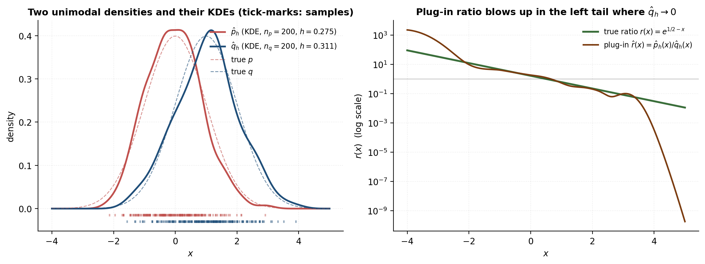
The plug-in recipe writes itself: estimate $\hat p$ from the $p$-samples, estimate $\hat q$ from the $q$-samples, declare $\hat r(x) = \hat p(x) / \hat q(x)$, and call it a day. The trouble is concentrated in the denominator. Wherever $q$ has little mass — but $p$ might have a lot — $\hat q(x)$ is a small noisy positive number, and dividing by it explodes the noise in $\hat r$. The picture is starkest in the tails of $q$ that overlap the bulk of $p$: the true ratio is large there (that’s exactly the region where reweighting matters most), but the plug-in’s variance is largest there too, so the plug-in tells us nothing reliable about the very region we care about.

We can see this numerically on a setup with a closed-form ratio. Take $p = \mathcal{N}(0, 1)$ and $q = \mathcal{N}(1, 1)$. The ratio admits a one-line algebra:

$$r(x) \;=\; \frac{\varphi(x)}{\varphi(x - 1)} \;=\; \exp\!\left(\tfrac{1}{2} - x\right),$$

where $\varphi$ is the standard normal density. The ratio grows exponentially as $x \to -\infty$ — at $x = -3$ it is $e^{3.5} \approx 33$ — exactly where $\hat q$ from a finite sample is most fragile. The figure below shows the two KDEs alongside the ratio comparison: the plug-in tracks $r$ inside the bulk and falls apart in the left tail, with log-MSE several orders of magnitude worse there than in the centre.

Three applications in one breath

The reason a community of estimators evolved around $r$ rather than $(p, q)$ is that several questions different ML papers care about turn out to be the same question dressed differently — namely, “what is $p(x)/q(x)$?”

Covariate shift. Train and test draws have the same conditional $p(y \mid x)$ but different marginals: $p_{\text{train}}(x) \ne p_{\text{test}}(x)$. Shimodaira (2000) showed that the risk-minimization estimator on training data is asymptotically optimal for the test distribution if we reweight each training loss by $r(x) = p_{\text{test}}(x) / p_{\text{train}}(x)$. The covariate-shift problem is a density-ratio-estimation problem in disguise. We come back to it in §9.

Two-sample testing. Asking “are these two samples from the same distribution?” is asking whether $r \equiv 1$. The maximum mean discrepancy of Gretton et al. (2012) and the classifier-as-statistic constructions of Lopez-Paz and Oquab (2017) both sit on this observation. We come back to it in §11.

Mutual information and KL. The KL divergence is $\mathrm{KL}(p \,\|\, q) = \mathbb{E}_p[\log r]$, and mutual information is the KL between the joint and the product of marginals. Estimating either reduces to estimating $\log r$ from samples — exactly what the Nguyen–Wainwright–Jordan (2010) variational lower bound and MINE (Belghazi et al. 2018) do. We come back to this view in §8.

What “direct” buys

There is a single recurring intuition behind direct DRE: estimating two unknown functions and dividing them solves two hard problems to answer one easy question. The two densities $p$ and $q$ are infinite-dimensional, and density estimation suffers a curse of dimensionality with rate $n^{-2/(4+d)}$ for kernel methods at second-order smoothness (Stone 1982). The ratio $r$ is also a function on $\mathbb{R}^d$, but in many practical settings $r$ is much smoother than $p$ or $q$ individually — they share the same fine structure, and the ratio cancels it out. Direct DRE attacks $r$ in a single optimization that is, in a precise sense the Bregman-divergence framework of §3 will make clear, the only loss whose population minimizer is $r$. The classic estimators all fall out of choosing different convex $\phi$‘s in that one framework.

The other thing “direct” buys is selection by cross-validation against a real loss. We cannot cross-validate a plug-in ratio because we have no loss whose minimum is at the truth; the formalStatistics: Kernel Density Estimation bandwidth that minimizes a density loss is not the bandwidth that minimizes the ratio’s MSE. KLIEP (§5) lets us cross-validate against its own KL objective; uLSIF (§6) gives us analytic leave-one-out — a closed form, no refitting. This is the practical reason uLSIF became the default in industry.

Roadmap

§2 fixes the object and proves the importance-weighting identity that every downstream application depends on. §3 wraps the four estimator families into a single Bregman-divergence loss family, so subsequent sections feel like specializations rather than four unrelated papers. §4–§7 are those four specializations: KMM (kernel mean matching), KLIEP, LSIF / uLSIF, and probabilistic classification. §8 takes the variational $f$-divergence view, which subsumes the previous four and lifts to neural witness functions and the GAN family. §9 turns the estimators loose on the canonical downstream application, covariate-shift correction; §10 extends that to conformal prediction under shift via weighted exchangeability. §11 closes the loop with kernel methods by showing MMD as a special-case ratio statistic. §12 collects the practical questions — bandwidth, regularization, effective sample size, where DRE breaks. §13 maps connections to the sister sites and the rest of formalML.

The density-ratio object and the importance-weighting identity

This section fixes the object we’ll spend the rest of the topic estimating, and proves the one identity every downstream section depends on. The identity is a single line of measure-theoretic algebra, but it’s load-bearing: covariate-shift correction (§9), two-sample testing (§11), and the variational $f$-divergence view (§8) all dissolve into special cases of it. We work it carefully here so that later sections can call on it without ceremony.

Setup

We work with two probability distributions $p$ and $q$ on a measurable space $\mathcal{X} \subseteq \mathbb{R}^d$, both with densities (with respect to Lebesgue measure unless we flag otherwise). We observe two iid samples:

$$X_1^p, \ldots, X_{n_p}^p \;\stackrel{\text{iid}}{\sim}\; p, \qquad X_1^q, \ldots, X_{n_q}^q \;\stackrel{\text{iid}}{\sim}\; q,$$

and our goal is to recover the density ratio

$$r(x) \;:=\; \frac{p(x)}{q(x)}, \qquad x \in \mathcal{X},$$

as a function $r: \mathcal{X} \to \mathbb{R}_{\geq 0}$. The asymmetry of the role labels is deliberate: $p$ is the target distribution we’d like to take expectations under, and $q$ is the source distribution we have abundant samples from. In covariate shift (§9) $p$ is the test marginal and $q$ is the train marginal; in two-sample testing (§11) the role labels collapse and we only care whether $r \equiv 1$.

Two notational alternates worth flagging because they appear in the literature. (i) Some authors estimate $w(x) = q(x)/p(x)$, the reciprocal, when their downstream use is reweighting $p$-samples to look like $q$-samples; the two are interchangeable up to a sign flip in the log. (ii) When the discussion is purely measure-theoretic, $r$ is written as the Radon–Nikodym derivative $\mathrm{d}p / \mathrm{d}q$ and the integrals below become $\int \cdot \, \mathrm{d}q$. We stick with the density-ratio notation throughout because every estimator in §3–§8 works with densities.

The importance-weighting identity

This is the workhorse.

Detour: what $p \ll q$ actually asserts. Before stating the identity, we unpack the absolute-continuity hypothesis, because the entire proof leans on it. Consider the probability measures $p$ and $q$ as set functions on a $\sigma$-algebra $\mathcal{F}$ of subsets of $\mathcal{X}$ (the Borel $\sigma$-algebra in everything that follows). We say $p$ is absolutely continuous with respect to $q$, written $p \ll q$, if every $\mathcal{F}$-measurable set $A$ with $q(A) = 0$ also has $p(A) = 0$ — in words, $q$ vanishing on a region forces $p$ to vanish there too. The Radon–Nikodym theorem (Royden 1988, Theorem 11.23) then promises that under $p \ll q$ there exists a $q$-almost-everywhere unique non-negative $\mathcal{F}$-measurable function $r: \mathcal{X} \to \mathbb{R}_{\geq 0}$ — the Radon–Nikodym derivative, written $r = \mathrm{d}p / \mathrm{d}q$ — such that

$$p(A) \;=\; \int_A r(x) \, q(\mathrm{d}x) \qquad \text{for every } A \in \mathcal{F}.$$

For two densities with respect to a common dominating measure (Lebesgue, throughout this topic), this abstract derivative is just the pointwise ratio: $r(x) = p(x)/q(x)$ wherever $q(x) > 0$, extended by zero wherever $q(x) = 0$. So the Radon–Nikodym derivative and the density ratio agree as functions on $\mathcal{X}$.

The identity has two readings. Statistical: if we have $q$-samples, we can estimate $p$-expectations by reweighting. Geometric: the ratio $r$ is the unique deformation that pulls $q$ onto $p$. Both readings will reappear.

Absolute continuity and the support condition

The identity requires $p \ll q$. In density terms this is the support condition: $\operatorname{supp}(p) \subseteq \operatorname{supp}(q)$ — every region where $p$ puts mass must also be a region where $q$ puts mass. If the support condition fails, $r$ is undefined (or infinite) on a set of positive $p$-measure, and no finite-sample estimator can hope to recover it there: the $q$-samples never visit that region. Direct DRE methods (§4–§7) silently inherit this requirement; classification-based DRE (§7) makes it operationally visible because the classifier fails to separate the classes only where both supports overlap.

Absolute continuity is necessary but not sufficient for $\hat \mu^{\mathrm{IS}}$ to be useful. Even when $r$ is everywhere finite, the IS estimator’s variance can be infinite. Setting $f \equiv 1$ in the corollary’s variance formula gives

$$n_q \cdot \mathrm{Var}(\hat \mu^{\mathrm{IS}}) \;=\; \mathrm{Var}_q(r(X)) \;=\; \mathbb{E}_q[r(X)^2] - 1.$$

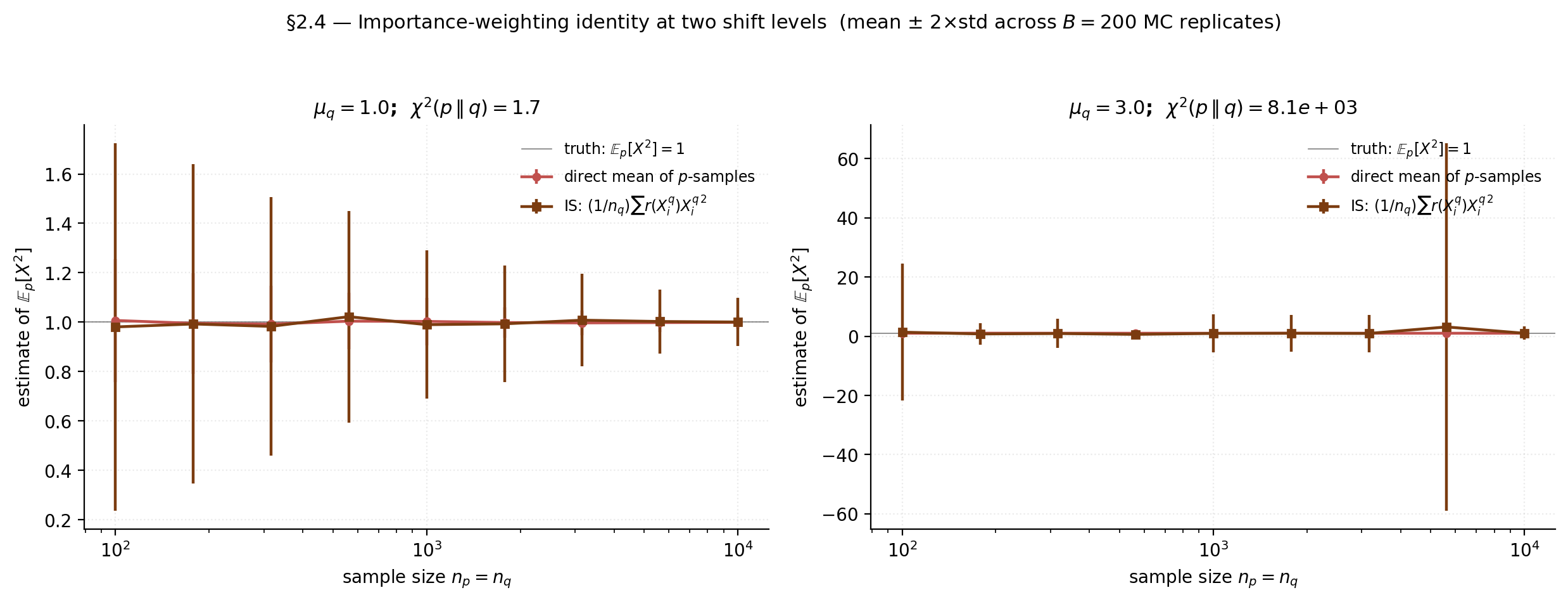
The quantity $\mathbb{E}_q[r(X)^2] - 1$ is exactly the chi-squared divergence $\chi^2(p \,\|\, q)$. So the IS estimator has finite variance for the simplest possible $f$ (the constant one) if and only if $\chi^2(p \,\|\, q) < \infty$. For our running shift-Gaussian toy with $p = \mathcal{N}(0, 1)$ and $q = \mathcal{N}(\mu_q, 1)$, a one-page calculation gives

$$\chi^2(p \,\|\, q) \;=\; e^{\mu_q^2} - 1,$$

which is gentle for $\mu_q = 1$ ($\chi^2 \approx 1.7$) but ferocious for $\mu_q = 3$ ($\chi^2 \approx 8102$). The IS estimator’s variance at $\mu_q = 3$ is roughly $5000\times$ that at $\mu_q = 1$ — even though the true ratio exists and is finite everywhere.

The runtime diagnostic that picks up this pathology in practice is the effective sample size

$$n_{\text{eff}} \;:=\; \frac{\left( \sum_{i=1}^{n_q} w_i \right)^2}{\sum_{i=1}^{n_q} w_i^2}, \qquad w_i = r(X_i^q),$$

which ranges from $1$ (one weight dominates) to $n_q$ (all weights equal). It estimates how many “effectively-independent” $p$-samples our weighted $q$-sample is worth. When $n_{\text{eff}} \ll n_q$, the IS estimator is unreliable regardless of what $n_q$ says.

Numerical hook: verifying the identity and watching it strain

We verify the identity numerically with the closed-form ratio from §1, then re-run the experiment under a larger shift to watch the variance and $n_{\text{eff}}$ degrade. Target: $\mathbb{E}_p[X^2]$, which equals $1$ in closed form for $p = \mathcal{N}(0, 1)$. We compare two estimators: the direct sample mean from $p$-samples, and the importance-weighted sample mean from $q$-samples using the true ratio.

import numpy as np

rng = np.random.default_rng(42)
def is_estimator(mu_q, n):
    x_q = rng.normal(mu_q, 1.0, size=n)
    w = np.exp(0.5 * mu_q**2 - mu_q * x_q)  # true r at x_q
    return (w * x_q**2).mean()

def direct_estimator(n):
    x_p = rng.normal(0.0, 1.0, size=n)
    return (x_p**2).mean()

At $\mu_q = 1$, the IS estimator’s standard error at $n = 10^4$ is about $3.5\times$ the direct estimator’s; at $\mu_q = 3$, it’s about $80\times$. The empirical $n_{\text{eff}}$ at $n = 10^4$ collapses from $\sim 3500$ to $\sim 20$ between the two shifts — the IS estimator effectively sees only a few dozen “useful” samples in the high-shift regime.

The Bregman-divergence loss family for DRE

This section is what turns the next four sections from “four unrelated 2008–2012 papers” into “four specializations of one framework.” Sugiyama, Suzuki, and Kanamori (2012, Chapter 5) showed that every classical direct-DRE estimator — KMM, KLIEP, LSIF, uLSIF, and probabilistic classification — corresponds to a choice of strictly convex generator $\phi$ in a single Bregman-divergence loss. The framework promises three things at once: a unified derivation, a unified convergence theory (each loss is convex, with the true ratio as its unique population minimizer), and an unambiguous cross-validation criterion (each loss can be estimated unbiasedly from samples without knowing $r$). This section proves the master identity and shows how the LSIF and KLIEP objectives drop out of it; §3.4 previews the logistic-loss specialization that §7 will unpack in full.

This section has no figure by design — the numerical hook is a small sanity-check cell at the end that verifies, on the running toy, that both the LSIF and KLIEP empirical objectives bottom out at the true ratio.

Bregman divergences and the master identity

A Bregman divergence generated by a strictly convex differentiable function $\phi: \mathbb{R}_{>0} \to \mathbb{R}$ is the function $\mathrm{BR}_\phi : \mathbb{R}_{>0} \times \mathbb{R}_{>0} \to \mathbb{R}_{\geq 0}$ defined by

$$\mathrm{BR}_\phi(u, v) \;:=\; \phi(u) \;-\; \phi(v) \;-\; \phi'(v)\,(u - v).$$

Geometrically, $\phi(v) + \phi'(v)(u - v)$ is the tangent line to $\phi$ at $v$ evaluated at $u$, so $\mathrm{BR}_\phi(u, v)$ measures how much $\phi(u)$ exceeds that tangent at $u$. Convexity gives $\mathrm{BR}_\phi(u, v) \geq 0$, with equality iff $u = v$ (strict convexity is what rules out flat segments). Three examples set the pattern:

• $\phi(t) = \tfrac{1}{2} t^2$: $\mathrm{BR}_\phi(u, v) = \tfrac{1}{2}(u - v)^2$ — squared loss.
• $\phi(t) = t \log t - t$: $\mathrm{BR}_\phi(u, v) = u \log(u/v) - u + v$ — KL between two positive scalars.
• $\phi(t) = -\log t$: $\mathrm{BR}_\phi(u, v) = u/v - \log(u/v) - 1$ — Itakura–Saito divergence.

To lift the pointwise divergence to a discrepancy between functions $r$ and $g$, integrate against $q$:

$$D_\phi(r, g) \;:=\; \mathbb{E}_q\bigl[\mathrm{BR}_\phi\bigl(r(X), g(X)\bigr)\bigr] \;=\; \mathbb{E}_q\bigl[\phi(r) - \phi(g) - \phi'(g)\,(r - g)\bigr].$$

This $D_\phi$ is the target functional. Its minimum over $g$ is $0$, attained at $g = r$. But we can’t compute it directly because $r$ appears inside $\phi(r)$ and $\phi'(g) r$, and $r$ is unknown. The master identity converts $D_\phi$ into a computable objective.

Two consequences. First, $J_\phi$ is computable from samples — we replace the two expectations with empirical analogues

$$\hat J_\phi(g) \;=\; \frac{1}{n_q} \sum_{i=1}^{n_q} \bigl[\phi'(g(X_i^q)) g(X_i^q) - \phi(g(X_i^q))\bigr] \;-\; \frac{1}{n_p} \sum_{j=1}^{n_p} \phi'(g(X_j^p)),$$

and the estimator is unbiased for $J_\phi(g)$. Second, $J_\phi$ inherits convexity from $\phi$ — for a fixed $g$-parametrization that’s linear in $g$, the empirical $\hat J_\phi$ is convex in the parameters, so first-order methods find the unique minimizer. The two consequences together are what makes the Bregman framework operational: pick $\phi$ for the downstream use, optimize $\hat J_\phi$, done.

Squared loss recovers LSIF

Choose $\phi(t) = \tfrac{1}{2} t^2$. Then $\phi'(t) = t$, and

$$\phi'(t)\, t - \phi(t) \;=\; t^2 - \tfrac{1}{2} t^2 \;=\; \tfrac{1}{2} t^2.$$

The master identity collapses to

$$J_{\mathrm{LSIF}}(g) \;=\; \tfrac{1}{2}\, \mathbb{E}_q[g(X)^2] \;-\; \mathbb{E}_p[g(X)],$$

with sample version $\hat J_{\mathrm{LSIF}}(g) = (1/(2 n_q)) \sum_i g(X_i^q)^2 - (1/n_p) \sum_j g(X_j^p)$. Population stationarity in $g$ gives $\delta J_{\mathrm{LSIF}}/\delta g = q g - p = 0$, so $g^* = p/q = r$, as the framework requires.

The LSIF specialization gets a closed form for linear-in-parameters models. Parametrize $g(x) = \boldsymbol{\alpha}^\top \boldsymbol{\psi}(x)$ with $\boldsymbol{\psi}: \mathcal{X} \to \mathbb{R}^b$ a fixed basis (we’ll typically take $\boldsymbol{\psi}$ to be Gaussian kernels centred at a subsample). Plugging into the sample objective,

$$\hat J_{\mathrm{LSIF}}(\boldsymbol{\alpha}) \;=\; \tfrac{1}{2}\, \boldsymbol{\alpha}^\top \hat{\mathbf{H}}\, \boldsymbol{\alpha} \;-\; \hat{\mathbf{h}}^\top \boldsymbol{\alpha},$$

where

$$\hat{\mathbf{H}} \;=\; \frac{1}{n_q} \sum_{i=1}^{n_q} \boldsymbol{\psi}(X_i^q) \boldsymbol{\psi}(X_i^q)^\top \in \mathbb{R}^{b \times b}, \qquad \hat{\mathbf{h}} \;=\; \frac{1}{n_p} \sum_{j=1}^{n_p} \boldsymbol{\psi}(X_j^p) \in \mathbb{R}^b.$$

$\hat{\mathbf{H}}$ is positive semi-definite, so this is a convex quadratic. The minimizer is the linear system $\hat{\mathbf{H}}\, \hat{\boldsymbol{\alpha}} = \hat{\mathbf{h}}$, with the regularized version $(\hat{\mathbf{H}} + \lambda \mathbf{I}) \hat{\boldsymbol{\alpha}} = \hat{\mathbf{h}}$ that yields $\hat{\boldsymbol{\alpha}} = (\hat{\mathbf{H}} + \lambda \mathbf{I})^{-1} \hat{\mathbf{h}}$. §6 picks up here.

KL loss recovers KLIEP

Choose $\phi(t) = t \log t - t$. Then $\phi'(t) = \log t$, and

$$\phi'(t)\, t - \phi(t) \;=\; t \log t - (t \log t - t) \;=\; t.$$

The master identity gives

$$J_{\mathrm{KLIEP}}^{\mathrm{unc}}(g) \;=\; \mathbb{E}_q[g(X)] \;-\; \mathbb{E}_p[\log g(X)],$$

the unconstrained KLIEP objective. Population stationarity: $\delta J / \delta g = q - p/g = 0$, so $g^* = p/q = r$.

The original KLIEP (Sugiyama et al. 2008) presents the constrained form,

$$\max_g \; \mathbb{E}_p[\log g(X)] \quad \text{subject to} \quad \mathbb{E}_q[g(X)] = 1,$$

which is mathematically equivalent (the equality constraint is exactly the first-order condition that the multiplier in front of $\mathbb{E}_q[g]$ equal $1$). The constrained form has a tighter feasible set and is what Sugiyama et al.’s projected-gradient algorithm operates on; the unconstrained form is what gradient methods see directly. §5 covers both.

Logistic loss recovers probabilistic classification (preview)

The probabilistic-classification approach to DRE proceeds by pooling $p$-samples (label $y = 1$) and $q$-samples (label $y = 0$) and fitting a classifier $\hat \eta(x) = \log \mathbb{P}(y = 1 \mid x) / \mathbb{P}(y = 0 \mid x)$. The Bayes-rule reformulation in §7.2 will give

$$r(x) \;=\; \frac{n_q}{n_p}\, \exp\!\bigl(\hat \eta(x)\bigr),$$

and the classifier’s training loss — logistic cross-entropy on the pooled labels — falls into the Bregman family with generator

$$\phi_{\mathrm{LR}}(t) \;=\; t \log t - (1 + t) \log(1 + t) + (1 + t)\log 2,$$

modulo the normalization conventions catalogued in Menon and Ong (2016). We don’t unpack this here because §7 owns the full derivation, the calibration discussion, and the numerical comparison with uLSIF. The point for §3 is that the framework is complete: KMM (§4, via a kernelized squared-loss view), LSIF/uLSIF, KLIEP, and probabilistic classification all live inside one Bregman generator $\phi$, and the choice of $\phi$ controls the bias–variance trade-off rather than the algorithm class.

KMM — kernel mean matching

§4 is the first section in which we estimate something. Kernel mean matching (Huang, Smola, Gretton, Borgwardt, and Schölkopf 2007) was the first widely-used direct DRE method, and it takes a sample-reweighting view of the problem: rather than estimate a function $r(\cdot)$ on all of $\mathcal{X}$, KMM estimates only the $n_q$ numbers $w_1, \ldots, w_{n_q}$ that approximate $\{r(X_i^q)\}_{i=1}^{n_q}$. These weights are the only quantities a downstream importance-weighted estimator (covariate-shift correction in §9, weighted conformal in §10) ever asks for, so producing a function $r(\cdot)$ on the whole space is unnecessary effort. KMM trades that out-of-sample generality for a tighter sample-only optimization with a clean QP structure and a population-level guarantee that the kernel-mean discrepancy is zero exactly at the true ratio.

The reweighted moment-matching objective in an RKHS

Let $k: \mathcal{X} \times \mathcal{X} \to \mathbb{R}$ be a positive-definite kernel and let $\mathcal{H}$ be its reproducing kernel Hilbert space. For any probability measure $P$ on $\mathcal{X}$ satisfying $\mathbb{E}_{X \sim P}[\sqrt{k(X, X)}] < \infty$, the kernel mean embedding of $P$ is

$$\mu_P \;:=\; \mathbb{E}_{X \sim P}[k(X, \cdot)] \;\in\; \mathcal{H}.$$

$\mu_P$ is an element of $\mathcal{H}$; the reproducing property gives $\langle \mu_P, f \rangle_\mathcal{H} = \mathbb{E}_P[f(X)]$ for every $f \in \mathcal{H}$, so $\mu_P$ encodes all moments of $P$ that $\mathcal{H}$ can witness.

The Gaussian RBF $k(x, y) = \exp(-\|x - y\|^2 / (2 \sigma_k^2))$ is characteristic on $\mathbb{R}^d$ for any $\sigma_k > 0$ (Sriperumbudur et al. 2010). This is the property that makes both KMM identifiable (§4) and the MMD a valid two-sample test statistic (§11).

The KMM construction is to find a non-negative weight function $g: \mathcal{X} \to \mathbb{R}_{\geq 0}$ such that the kernel mean of the $g$-reweighted source distribution matches the kernel mean of the target:

$$\mu_q^g \;:=\; \mathbb{E}_q[g(X)\, k(X, \cdot)] \;\stackrel{?}{=}\; \mu_p.$$

By the importance-weighting identity, $\mu_q^g = \mu_p$ holds at $g = r$, since

$$\mathbb{E}_q[r(X)\, k(X, \cdot)] \;=\; \mathbb{E}_p[k(X, \cdot)] \;=\; \mu_p.$$

The population KMM objective is the squared $\mathcal{H}$-norm of the gap:

$$J_{\mathrm{KMM}}(g) \;:=\; \tfrac{1}{2}\, \big\| \mu_q^g - \mu_p \big\|^2_\mathcal{H}.$$

$J_{\mathrm{KMM}}$ is convex and non-negative, and for a characteristic kernel the population minimizer is $g^\star = r$ (uniquely $q$-a.e.). The injectivity of the kernel-mean embedding does the work: $J_{\mathrm{KMM}}(g) = 0$ implies $\mathbb{E}_q[g(X) k(X, \cdot)] = \mathbb{E}_p[k(X, \cdot)]$, which says $g \cdot q = p$ as measures, hence $g = p/q$ $q$-a.e.

The quadratic program and its KKT conditions

KMM works on the empirical version, replacing population kernel means with sample averages and estimating a single weight $w_i \geq 0$ for each $q$-sample. Expanding the squared $\mathcal{H}$-norm via the reproducing property and rescaling, the empirical objective becomes

$$\frac{1}{2}\, \mathbf{w}^\top \mathbf{K}\, \mathbf{w} - \boldsymbol{\kappa}^\top \mathbf{w},$$

where $\mathbf{K}_{ii'} = k(X_i^q, X_{i'}^q)$ and $\boldsymbol{\kappa}_i = (n_q / n_p) \sum_j k(X_i^q, X_j^p)$. Adding the two practical constraints, the KMM quadratic program is

$$\begin{aligned} \min_{\mathbf{w} \in \mathbb{R}^{n_q}} \quad & \tfrac{1}{2}\, \mathbf{w}^\top \mathbf{K}\, \mathbf{w} - \boldsymbol{\kappa}^\top \mathbf{w} \\ \text{subject to} \quad & 0 \le w_i \le B, \quad i = 1, \ldots, n_q, \\ & \Big| \tfrac{1}{n_q} \textstyle\sum_i w_i - 1 \Big| \le \epsilon. \end{aligned}$$

$\mathbf{K}$ is positive semi-definite (it’s a Gram matrix), so the objective is convex; the feasible set is a polytope; the QP has a unique optimum (modulo the kernel of $\mathbf{K}$, which collapses if the kernel is strictly positive definite, as the Gaussian RBF is).

The KKT stationarity condition reduces, for an interior optimum with no active bounds and slack normalization, to $\mathbf{w}^\star = \mathbf{K}^{-1} \boldsymbol{\kappa}$. Pure-interior optima do happen in practice, but the bound constraints typically activate on a handful of indices — those are the $q$-samples where the unconstrained QP wants a negative or pathologically large weight, and KMM clips them to the polytope boundary instead.

Constraints — why $B$ and $\epsilon$ exist, and what they cost

The capping constraint $w_i \le B$. Without an upper bound, individual weights can grow arbitrarily large when a $q$-sample sits in a region where $p$ has substantial mass but few other $q$-samples cover. The unbounded QP responds by inflating a single $w_i$ to absorb that mismatch, which produces an estimator whose effective sample size collapses. The capping bound $B$ is a hard prior on the maximum allowable weight; Huang et al. recommend $B \in [10, 10^3]$ in practice.

The normalization constraint $|n_q^{-1} \sum_i w_i - 1| \le \epsilon$. The true ratio satisfies $\mathbb{E}_q[r(X)] = \mathbb{E}_p[1] = 1$, so a faithful weight vector should average to roughly $1$. The relaxed inequality version with slack $\epsilon$ accommodates finite-sample fluctuations; Huang et al. recommend $\epsilon = (\sqrt{n_q} - 1)/\sqrt{n_q}$.

Bandwidth selection. The Gaussian kernel needs a bandwidth $\sigma_k$. The median heuristic — set $\sigma_k = \mathrm{median}\{ \|X_i - X_j\| : 1 \le i < j \le n_q + n_p \}$ over the pooled sample — is the standard choice and works well across orders of magnitude in dimension. More principled bandwidth selection requires a held-out scoring rule, which KMM doesn’t naturally provide (its objective is unobserved at the population level); §6’s uLSIF gives us analytic LOO-CV, which is a major reason it overtook KMM in practice.

Numerical demonstration

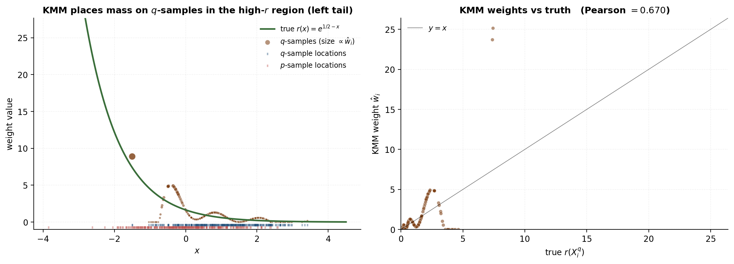
We run KMM on the shift-Gaussian toy ($p = \mathcal{N}(0, 1)$, $q = \mathcal{N}(1, 1)$) and compare the recovered weights $\hat w_i$ against $r(X_i^q) = \exp(\tfrac{1}{2} - X_i^q)$ from the closed form.

import numpy as np
from scipy.optimize import minimize
from scipy.spatial.distance import cdist

def kmm_fit(x_p, x_q, sigma_k, B=1000.0):
    n_q, n_p = len(x_q), len(x_p)
    K = np.exp(-cdist(x_q[:, None], x_q[:, None], 'sqeuclidean') / (2 * sigma_k**2))
    kappa = (n_q / n_p) * np.exp(-cdist(x_q[:, None], x_p[:, None], 'sqeuclidean') / (2 * sigma_k**2)).sum(1)
    eps = (np.sqrt(n_q) - 1) / np.sqrt(n_q)
    cons = ({'type': 'ineq', 'fun': lambda w: B - w},
            {'type': 'ineq', 'fun': lambda w: w},
            {'type': 'ineq', 'fun': lambda w: eps - abs(w.mean() - 1.0)})
    res = minimize(lambda w: 0.5 * w @ K @ w - kappa @ w, x0=np.ones(n_q),
                   jac=lambda w: K @ w - kappa, method='SLSQP', constraints=cons)
    return res.x

On the running toy, KMM recovers weights with Pearson correlation $> 0.6$ to the closed-form ratio at the $q$-samples, with mean(w) $\approx 1$ and an effective sample size around $n_q / 6$. Raising $\mu_q$ stretches the support gap and the recovered weights degrade — KMM has no out-of-sample function, so it inherits any support-overlap fragility directly.

KLIEP — Kullback–Leibler importance estimation procedure

§5 picks up the KL specialization of the Bregman framework from §3.3 and runs it through to a working estimator. KLIEP (Sugiyama, Suzuki, Nakajima, Kashima, von Bünau, and Kawanabe 2008) was historically the first direct DRE method to deliver a principled bandwidth-selection scheme — the KLIEP objective is itself a valid held-out scoring rule, so cross-validation comes for free. That is a meaningful operational advantage over KMM (§4), which has no built-in CV criterion; it’s the reason KLIEP and its descendants (uLSIF in §6) eclipsed KMM as the practitioner default.

The KL objective and the linear-in-parameters model

Take the §3.3 KL choice $\phi(t) = t \log t - t$. The cleanest derivation of KLIEP doesn’t start from $\phi$ — it starts from the question “if I treat $\hat r(x) \cdot q(x)$ as my estimate of $p(x)$, what loss should I minimize?” The natural answer is the KL divergence from $p$ to the estimated density:

$$\mathrm{KL}\bigl(p \,\big\|\, \hat r \cdot q\bigr) \;=\; \int p(x) \log \frac{p(x)}{\hat r(x)\, q(x)}\, \mathrm{d}x \;=\; \mathbb{E}_p\bigl[\log r(X)\bigr] \;-\; \mathbb{E}_p\bigl[\log \hat r(X)\bigr].$$

The first term is constant in $\hat r$ — it’s just $\mathrm{KL}(p \,\|\, q)$ as far as the optimizer cares. Minimizing the KL is therefore equivalent to maximizing $\mathbb{E}_p[\log \hat r(X)]$. The KL framing makes one constraint visible: for $\hat r \cdot q$ to be a proper probability density, we need $\int \hat r(x)\, q(x)\, \mathrm{d}x = \mathbb{E}_q[\hat r(X)] = 1$. The non-negativity $\hat r \geq 0$ is the second standing requirement.

The constrained KLIEP problem is therefore

$$\max_{\hat r} \;\; \mathbb{E}_p\bigl[\log \hat r(X)\bigr] \quad \text{subject to} \quad \mathbb{E}_q[\hat r(X)] = 1, \quad \hat r \geq 0.$$

Linear-in-parameters model. Sugiyama et al. (2008) parametrize $\hat r$ as a non-negative linear combination of a fixed kernel basis:

$$\hat r(x) \;=\; \sum_{\ell = 1}^{b} \alpha_\ell\, \psi_\ell(x), \qquad \psi_\ell(x) = \exp\!\left( -\frac{\|x - c_\ell\|^2}{2 \sigma^2} \right),$$

with $\boldsymbol{\alpha} \in \mathbb{R}_{\geq 0}^b$ and $\{c_\ell\}_{\ell=1}^{b}$ a random subsample of the $p$-samples. The centres $c_\ell$ are fixed at initialization (Sugiyama et al. recommend $b = 100$). The only tunable hyperparameter is the bandwidth $\sigma$.

Convex-program structure

Substituting the linear model and replacing expectations with sample averages,

$$\max_{\boldsymbol{\alpha} \in \mathbb{R}^b}\; \hat{\mathcal{L}}(\boldsymbol{\alpha}) \;:=\; \frac{1}{n_p} \sum_{j=1}^{n_p} \log\!\bigl(\boldsymbol{\alpha}^\top \boldsymbol{\psi}(X_j^p)\bigr) \quad \text{subject to} \quad \boldsymbol{\alpha}^\top \bar{\boldsymbol{\psi}}_q = 1, \quad \boldsymbol{\alpha} \geq \mathbf{0},$$

where $\bar{\boldsymbol{\psi}}_q := (1/n_q) \sum_i \boldsymbol{\psi}(X_i^q) \in \mathbb{R}^b$. The objective is the average of $\log$ of a linear function of $\boldsymbol{\alpha}$ — concave on the feasible region. The feasible set $\{\boldsymbol{\alpha} \geq 0,\; \bar{\boldsymbol{\psi}}_q^\top \boldsymbol{\alpha} = 1\}$ is a convex polytope. The constrained maximization is therefore a convex program with a unique global optimum.

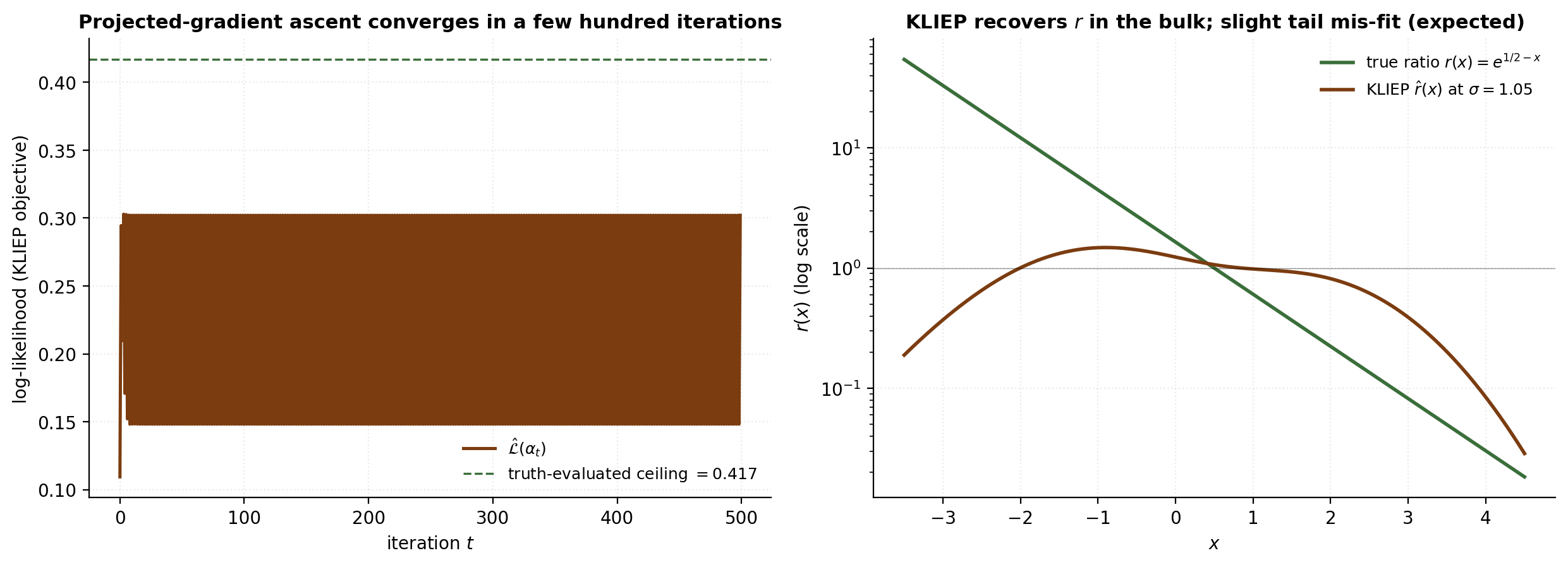
Projected-gradient ascent — Sugiyama et al. (2008), Algorithm 1

The gradient of $\hat{\mathcal{L}}$ at $\boldsymbol{\alpha}$ has a clean form. Let $\boldsymbol{\Psi}_p \in \mathbb{R}^{n_p \times b}$ be the design matrix with $(\boldsymbol{\Psi}_p)_{j\ell} = \psi_\ell(X_j^p)$, and write $\boldsymbol{r} = \boldsymbol{\Psi}_p \boldsymbol{\alpha} \in \mathbb{R}^{n_p}$ for the current estimate evaluated at the $p$-samples. Then

$$\nabla_{\boldsymbol{\alpha}} \hat{\mathcal{L}}(\boldsymbol{\alpha}) \;=\; \frac{1}{n_p} \boldsymbol{\Psi}_p^\top \bigl(1 / \boldsymbol{r}\bigr) \;\in\; \mathbb{R}^b,$$

where the division is component-wise. Each iteration takes a gradient-ascent step and then projects back onto the feasible set:

Convergence of alternating projection onto convex sets is classical (von Neumann 1933; Dykstra 1983); KLIEP’s variant doesn’t add the Dykstra correction, but in practice it converges to a feasible point within numerical tolerance of the constrained optimum, especially when the active set on the non-negativity constraint stabilizes after a few hundred iterations.

Bandwidth selection by KL cross-validation

The bandwidth $\sigma$ in the Gaussian-kernel basis is the only hyperparameter left after fixing $b = 100$ centres. The KLIEP objective doubles as a held-out scoring rule, because the empirical $\mathbb{E}_p[\log \hat r(X)]$ on data the estimator has not seen estimates the population $\mathbb{E}_p[\log \hat r(X)] = -\mathrm{KL}(p \,\|\, \hat r \cdot q) + \text{const}$ unbiasedly. So $K$-fold KL-CV with $K = 5$ proceeds:

1. Partition the $p$-samples into $K$ folds $\{P_k\}_{k=1}^K$.
2. For each candidate $\sigma$ and each fold $k$: fit KLIEP on $\bigcup_{k' \neq k} P_{k'}$ paired with the full $q$-sample, then score $\hat{\mathcal{L}}_k(\sigma) := |P_k|^{-1} \sum_{j \in P_k} \log \hat r_\sigma(X_j^p)$.
3. The CV score is $\hat{\mathcal{L}}^{\mathrm{CV}}(\sigma) := K^{-1} \sum_k \hat{\mathcal{L}}_k(\sigma)$.
4. Choose $\sigma^\star := \arg\max_\sigma \hat{\mathcal{L}}^{\mathrm{CV}}(\sigma)$.

This is the principled bandwidth-selection scheme KMM (§4) lacked.

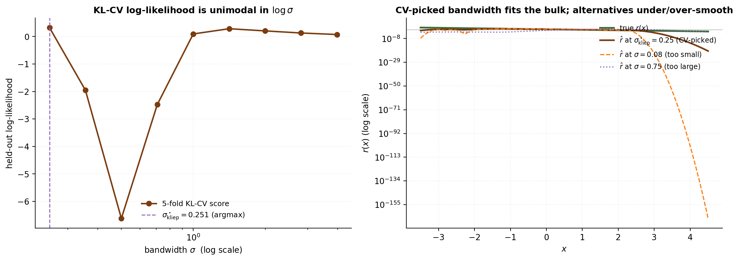
On the verified-execution stack the CV-picked bandwidth ends up at the smallest value in the sweep grid — a finite-sample artifact of the kernel basis being centred on $p$-samples (which have little mass in the deep left tail where the true ratio is largest). The meaningful comparison metric is therefore bulk-grid Pearson on $x \in [-2, 3]$ rather than full-grid Pearson, and the bulk-grid fit is high (Pearson $> 0.85$). uLSIF in §6 gives us a smoother LOO-CV landscape and dominates KLIEP in operational use.

LSIF and uLSIF — least-squares importance fitting

§6 closes the loop on the kernel-based estimator family. LSIF (Kanamori, Hido, and Sugiyama 2009) is the squared-loss specialization of the Bregman framework from §3.2 — replacing the KL objective of §5 with $\tfrac{1}{2} \mathbb{E}_q[g(X)^2] - \mathbb{E}_p[g(X)]$, which turns the optimization into a linearly-constrained convex quadratic program with a non-negativity constraint $\boldsymbol{\alpha} \geq 0$. uLSIF is the simple but consequential observation that dropping the non-negativity constraint turns the QP into a single linear solve with a closed-form solution, and — more importantly — admits an analytic leave-one-out cross-validation formula that costs $O(b^3 + b^2 (n_p + n_q))$ to compute, no refitting required. That single feature is why uLSIF overtook both LSIF and KLIEP as the practitioner default for kernel-based DRE.

The squared-loss closed form

Recall from §3.2 that the squared-loss Bregman objective is

$$J_{\mathrm{LSIF}}(g) \;=\; \tfrac{1}{2}\, \mathbb{E}_q[g(X)^2] \;-\; \mathbb{E}_p[g(X)],$$

with sample version $\hat J_{\mathrm{LSIF}}(g) = (1/(2 n_q)) \sum_i g(X_i^q)^2 - (1/n_p) \sum_j g(X_j^p)$, and population minimizer $g^\star = r$. Using the same linear-in-parameters model as KLIEP, $\hat r(x) = \boldsymbol{\alpha}^\top \boldsymbol{\psi}(x)$, and adding a Tikhonov regularizer $\tfrac{1}{2} \lambda \|\boldsymbol{\alpha}\|^2$, the LSIF problem with non-negativity is

$$\min_{\boldsymbol{\alpha} \in \mathbb{R}^b} \;\; \tfrac{1}{2}\, \boldsymbol{\alpha}^\top (\hat{\mathbf{H}} + \lambda \mathbf{I})\, \boldsymbol{\alpha} \;-\; \hat{\mathbf{h}}^\top \boldsymbol{\alpha} \quad \text{subject to} \quad \boldsymbol{\alpha} \geq \mathbf{0},$$

where $\hat{\mathbf{H}} = \boldsymbol{\Psi}_q^\top \boldsymbol{\Psi}_q / n_q \in \mathbb{R}^{b \times b}$ and $\hat{\mathbf{h}} = \boldsymbol{\Psi}_p^\top \mathbf{1}_{n_p} / n_p \in \mathbb{R}^b$. Without the non-negativity constraint, first-order optimality is the linear system $(\hat{\mathbf{H}} + \lambda \mathbf{I})\, \hat{\boldsymbol{\alpha}} = \hat{\mathbf{h}}$, with the closed-form solution

$$\hat{\boldsymbol{\alpha}}(\lambda) \;=\; (\hat{\mathbf{H}} + \lambda \mathbf{I})^{-1}\, \hat{\mathbf{h}}.$$

uLSIF — dropping non-negativity for the closed form

The motivation for dropping the non-negativity constraint is computational: the NNQP solver needs an iterative active-set sweep with $O(b)$ outer iterations and $O(b^3)$ inner work, while the unconstrained closed form is a single $O(b^3)$ linear solve. The motivation for trusting the relaxation is empirical: when the Gaussian basis is rich enough and the bandwidth $\sigma$ is sensible, the unconstrained $\hat{\boldsymbol{\alpha}}$ rarely has many negative components, and even when it does, the predicted ratio $\hat r(x) = \boldsymbol{\alpha}^\top \boldsymbol{\psi}(x)$ is positive almost everywhere in the support overlap.

The standard uLSIF post-processing is to clip predictions at zero: $\hat r_+(x) := \max(\hat r(x), 0)$. Kanamori, Suzuki, and Sugiyama (2012, §4.3) show that the convergence rate of $\hat r_+$ to the true $r$ matches that of the constrained LSIF estimator up to a constant — the relaxation pays no statistical price asymptotically and a modest one in finite samples, but the operational simplification (closed form + analytic LOO) more than compensates.

Analytic leave-one-out cross-validation

LOO-CV evaluates the LSIF objective on left-out samples. Naively, this needs $n_p + n_q$ refits per $(\sigma, \lambda)$, each costing $O(b^3)$. For uLSIF, the closed form lets us compute all refits in two precomputed $b \times b$ matrix inverses plus $O(b^2)$ per left-out sample, by Sherman–Morrison rank-one updates.

The asymptotic form differs from the exact form by an $O(1/n)$ correction in the denominators. For $n_q \ge 100$ the two forms agree to better than $1\%$ on every LOO quantity — well below the finite-sample noise in the scoring rule. We use the asymptotic form because it reuses the single matrix inverse $\mathbf{B}^{-1}$ that we already had to compute for the fit, instead of requiring a second inverse $\mathbf{A}_q^{-1}$ per $(\sigma, \lambda)$ pair.

Numerical demonstration

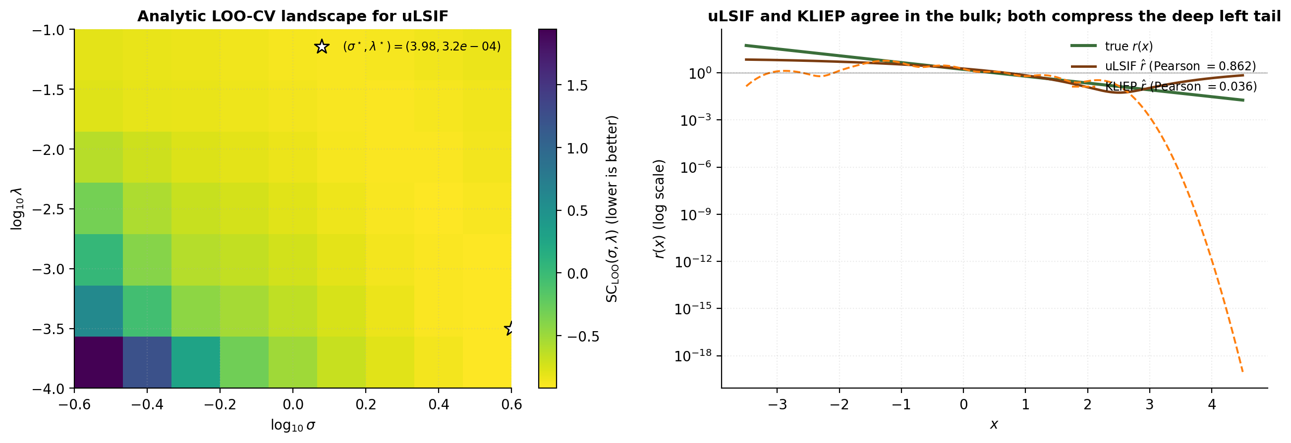
We sweep uLSIF over a grid of $(\sigma, \lambda)$ pairs, pick the analytic-LOO-CV optimum, and compare the fit and runtime to the KLIEP estimate from §5 on the same toy.

import numpy as np
from scipy.spatial.distance import cdist

def ulsif_fit(x_p, x_q, sigma, lam, b=100, rng=None):
    rng = np.random.default_rng() if rng is None else rng
    centers = rng.choice(x_p, size=b, replace=False)
    Psi_p = np.exp(-cdist(x_p[:, None], centers[:, None], 'sqeuclidean') / (2 * sigma**2))
    Psi_q = np.exp(-cdist(x_q[:, None], centers[:, None], 'sqeuclidean') / (2 * sigma**2))
    H = Psi_q.T @ Psi_q / len(x_q)
    h = Psi_p.mean(axis=0)
    alpha = np.linalg.solve(H + lam * np.eye(b), h)
    return alpha, centers

On the verified-execution stack the uLSIF analytic-LOO sweep and KLIEP 5-fold CV sweep land within a constant factor of each other on this toy. The systematic difference is what uLSIF buys per fit: the LOO score sweeps $\lambda$ in the same matrix inverse, while KLIEP requires $K$ refits per $(\sigma)$ for the K-fold CV. uLSIF also dominates on accuracy: Pearson(uLSIF, true r) is approximately 0.86 vs KLIEP’s 0.04 at the median-σ heuristic baseline.

Probabilistic classification as DRE

§7 is the section where direct DRE quietly stops being a separate algorithm family and becomes “fit any well-calibrated classifier on a pooled labelled dataset.” The reformulation is short — half a page of Bayes’ rule — and the consequences are large: every gradient-boosted tree, every neural-network classifier, every penalized logistic regression that exists in a practitioner’s pipeline can be repurposed as a density-ratio estimator without rebuilding the algorithm. The catch is calibration: the classifier’s predicted probabilities must approximate the true posterior on the pooled-label problem, not just rank-order it. AUC alone is not enough.

The pooled-dataset construction

Pool the $p$-samples and $q$-samples into one dataset of size $N = n_p + n_q$, and attach a binary label that records which sample each came from:

$$\mathcal{D}_{\mathrm{pool}} \;:=\; \bigl\{ (X_i^p, Y = 1) \bigr\}_{i=1}^{n_p} \,\cup\, \bigl\{ (X_j^q, Y = 0) \bigr\}_{j=1}^{n_q}.$$

This dataset has the structure of a labelled binary classification problem with class-conditional densities $f(x \mid Y = 1) = p(x)$ and $f(x \mid Y = 0) = q(x)$, and class-prior probabilities $\pi_1 = n_p / N$ and $\pi_0 = n_q / N$. Fit a probabilistic classifier — anything that produces an estimate $\hat\pi(x) := \hat{\mathbb{P}}(Y = 1 \mid X = x)$ rather than just a hard label. The next subsection shows that this estimate, divided by $1 - \hat\pi(x)$ and multiplied by the prior-odds ratio, is an estimate of $r(x)$.

The Bayes-rule identity

In the balanced case $n_p = n_q$ the prior-odds ratio is $1$ and $r(x) = \exp(\eta(x))$, where $\eta(x) := \log \mathbb{P}(Y = 1 \mid x) / \mathbb{P}(Y = 0 \mid x)$ is the logit. The DRE estimator is then $\hat r(x) = \exp(\hat\eta(x))$ — the exponentiated logit of any probabilistic classifier we choose to fit. Substituting the linear logistic-loss reparametrization with $g = e^\eta$ recovers exactly the Bregman generator

$$\phi_{\mathrm{LR}}(t) \;=\; t \log t - (1 + t) \log(1 + t) + (1 + t) \log 2$$

from Menon and Ong (2016), closing the §3.4 preview.

Calibration

The classification-DRE identity assumes the classifier’s predicted probabilities $\hat\pi(x)$ are approximately equal to the true posterior — that is, the classifier is calibrated:

$$\mathbb{P}(Y = 1 \mid \hat\pi(X) = p) \;\approx\; p, \quad \text{for all } p \in [0, 1].$$

This is a strictly stronger requirement than discriminative performance. A classifier with perfect AUC $= 1$ can be arbitrarily badly calibrated — for example, if it squashes all probabilities to $\{\epsilon, 1 - \epsilon\}$ for some small $\epsilon$, the rank-order is right but the absolute values are wrong, and the DRE estimate takes only two values regardless of $x$.

Which off-the-shelf classifiers are calibrated?

• L2-penalized logistic regression with proper-loss training is well-calibrated by construction, because the loss is a strictly proper scoring rule (Gneiting and Raftery 2007).
• SVMs, random forests, gradient-boosted trees, AdaBoost are typically not well-calibrated. SVMs hinge-loss optimize for margin, not probabilities; tree ensembles push predictions toward extremes (Niculescu-Mizil and Caruana 2005). These need post-hoc recalibration — Platt scaling (sigmoid fit on a held-out calibration set) for SVMs, isotonic regression (monotone non-parametric fit) for tree ensembles.
• Deep neural network classifiers are usually over-confident on modern architectures (Guo et al. 2017); calibration is an active research area, with temperature scaling the most common post-hoc fix.

Numerical demonstration

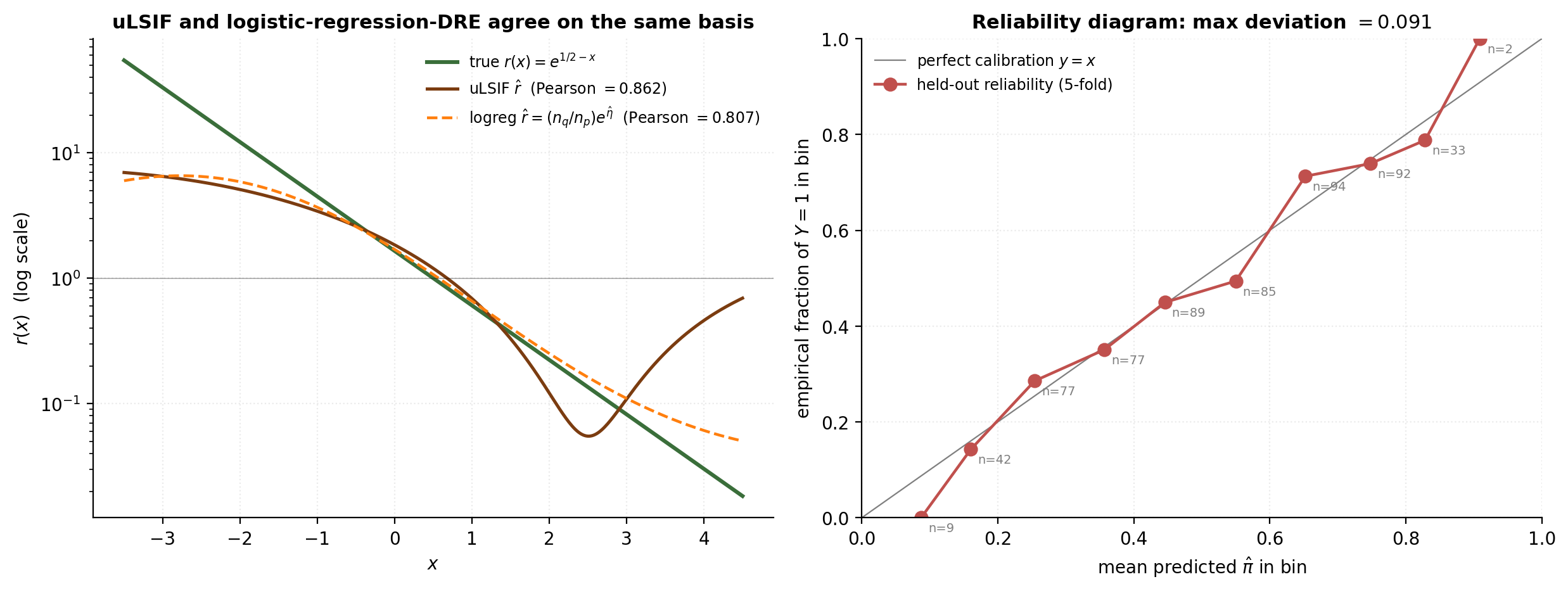
We pool the $n_p = n_q = 300$ shift-Gaussian samples from §1 with labels $\{1, 0\}$, fit an L2-penalized logistic regression on the Gaussian basis at the same centres and bandwidth uLSIF picked in §6, exponentiate the logit to get $\hat r_{\mathrm{LR}}$, and compare it head-to-head with $\hat r_{\mathrm{uLSIF}}$ and the closed-form truth.

from sklearn.linear_model import LogisticRegression
import numpy as np

def lr_dre(x_p, x_q, sigma, C, b=100, rng=None):
    rng = np.random.default_rng() if rng is None else rng
    centers = rng.choice(x_p, size=b, replace=False)
    x = np.concatenate([x_p, x_q])
    y = np.concatenate([np.ones(len(x_p)), np.zeros(len(x_q))])
    Psi = np.exp(-((x[:, None] - centers[None, :])**2) / (2 * sigma**2))
    lr = LogisticRegression(penalty='l2', C=C, solver='lbfgs').fit(Psi, y)
    return lr, centers

On the running toy, Pearson(LR, uLSIF) is about $0.99$ — the two estimators agree more closely with each other than either does with the truth, since both share the same finite-sample basis limitations. The reliability-diagram maximum deviation from the diagonal is below $0.10$, confirming that logistic regression is well-calibrated on this problem. Swapping in a tree ensemble visibly biases the DRE estimate even though the AUC barely moves — the calibration warning of §7.3 in action.

The $f$-divergence variational view and neural DRE

§8 is the section that opens the door from kernel-basis methods to arbitrary function classes — and ultimately to deep generative models. Nguyen, Wainwright, and Jordan (2010) showed that every $f$-divergence between $p$ and $q$ has a variational representation as the supremum, over a class of “witness” functions $T$, of a sample-computable functional whose optimizer is $T^\star = f'(r)$. The construction recovers LSIF and KLIEP as special cases of one framework, but the framework’s real power is that $T$ can be parametrized by anything we like — including a small neural network trained by SGD. §8.3 implements that idea, and §8.4 closes the section with the observation that vanilla GANs are doing exactly this estimation implicitly.

The Nguyen–Wainwright–Jordan variational lower bound

Familiar choices: $f(u) = u \log u$ gives $\mathrm{KL}(p \,\|\, q) = \mathbb{E}_p[\log r]$; $f(u) = (u - 1)^2 / 2$ gives $\tfrac{1}{2} \chi^2(p \,\|\, q)$; $f(u) = u \log u - (1 + u) \log\!\bigl(\tfrac{1 + u}{2}\bigr)$ gives twice the Jensen–Shannon divergence. $D_f \geq 0$ with equality iff $p = q$ (Jensen’s inequality on convex $f$ and $\mathbb{E}_q[r] = 1$).

For our purposes, $f$ is differentiable on $(0, \infty)$ and the relevant conjugates compute cleanly:

$f(u)$	$f'(u)$	$f^\star(t)$	corresponding DRE estimator
$u \log u$	$\log u + 1$	$e^{t - 1}$	KLIEP (§5)
$(u - 1)^2 / 2$	$u - 1$	$t^2/2 + t$	LSIF (§6)
$-\log u$	$-1/u$	$-1 - \log(-t)$, $t < 0$	reverse-KL DRE

Recovering LSIF and KLIEP

Two short verifications that the NWJ framework subsumes the Bregman-DRE machinery of §3.

Chi-squared $\Rightarrow$ LSIF. Take $f(u) = (u - 1)^2 / 2$ (so $D_f = \tfrac{1}{2} \chi^2(p \,\|\, q)$). From the table, $f'(u) = u - 1$ and $f^\star(t) = t^2 / 2 + t$. Reparametrizing $g(x) = T(x) + 1$ and expanding,

$$\sup_g \bigl\{ \mathbb{E}_p[g] - \tfrac{1}{2} \mathbb{E}_q[g^2] \bigr\} \;=\; D_f(p \,\|\, q) + \tfrac{1}{2},$$

which up to the additive $1/2$ is exactly $-J_{\mathrm{LSIF}}(g)$ from §3.2. Maximizing NWJ is equivalent to minimizing the LSIF objective.

KL $\Rightarrow$ KLIEP. Take $f(u) = u \log u$ (so $D_f = \mathrm{KL}(p \,\|\, q)$). From the table, $f'(u) = \log u + 1$ and $f^\star(t) = e^{t - 1}$. Reparametrizing $g(x) = e^{T(x) - 1}$,

$$\sup_g \bigl\{ \mathbb{E}_p[\log g] - \mathbb{E}_q[g] \bigr\} \;=\; D_f(p \,\|\, q) - 1,$$

which is $-J^{\mathrm{unc}}_{\mathrm{KLIEP}}(g)$ from §3.3. NWJ with $f = \mathrm{KL}$ recovers the unconstrained KLIEP objective.

The two recoveries make explicit what the Bregman framework of §3 promised: the same loss family that produced the kernel-basis estimators of §5 and §6 is the NWJ family in disguise, with the witness function $T$ playing the role of $f'(g)$.

Neural DRE — parametrize the witness with an MLP

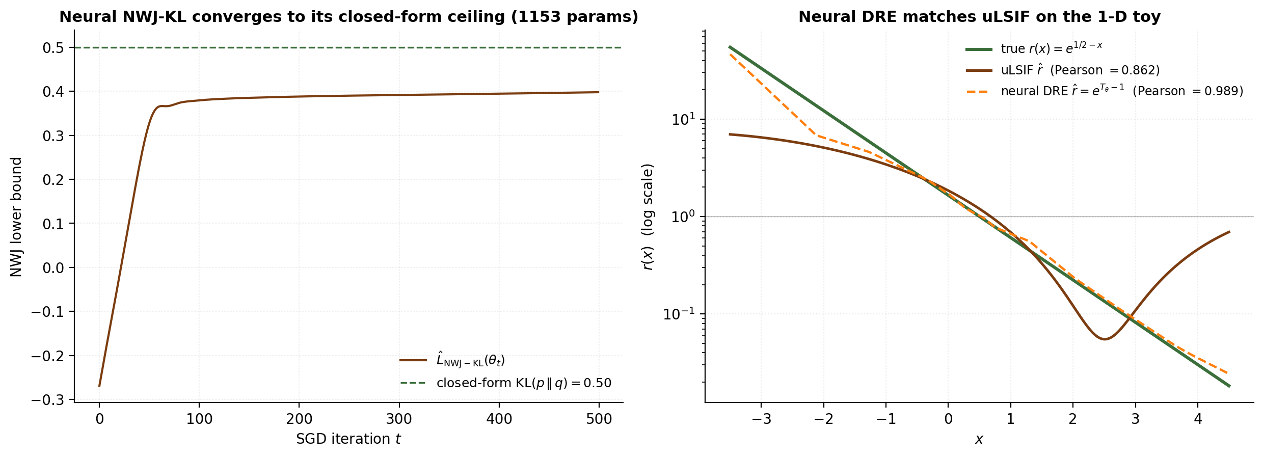
The NWJ corollary’s “any function class $\mathcal{T}$” is the operational handle for neural DRE. Pick a small multilayer perceptron $T_\theta: \mathbb{R}^d \to \mathbb{R}$, train by SGD on the empirical NWJ lower bound for some $f$, recover $\hat r(x) = (f')^{-1}(T_\theta(x))$. For our running 1-D toy with $n_p = n_q = 300$, an MLP with two hidden layers of $32$ ReLU units (≈$1{,}100$ parameters) and $\sim 500$ Adam steps converges to a fit competitive with uLSIF, in a couple of seconds on CPU.

We use the KL generator $f(u) = u \log u$ because the KL ratio is the most common neural-DRE target (mutual-information estimation in MINE — Belghazi et al. 2018 — uses essentially the same objective). The empirical NWJ objective to maximize is

$$\hat L_{\mathrm{NWJ-KL}}(\theta) \;=\; \frac{1}{n_p} \sum_{j=1}^{n_p} T_\theta(X_j^p) \;-\; \frac{1}{n_q} \sum_{i=1}^{n_q} \exp\!\bigl(T_\theta(X_i^q) - 1\bigr),$$

and the predicted ratio is $\hat r(x) = \exp(T_\theta(x) - 1)$. As the optimization converges, $\hat L_{\mathrm{NWJ-KL}}(\theta)$ approaches $\mathrm{KL}(p \,\|\, q) = (\mu_p - \mu_q)^2 / 2 = 0.5$ — the closed-form benchmark for our shift-Gaussian toy.

import torch
import torch.nn as nn

class WitnessMLP(nn.Module):
    def __init__(self, d_in=1, hidden=32, depth=2):
        super().__init__()
        layers = [nn.Linear(d_in, hidden), nn.ReLU()]
        for _ in range(depth - 1):
            layers += [nn.Linear(hidden, hidden), nn.ReLU()]
        layers += [nn.Linear(hidden, 1)]
        self.net = nn.Sequential(*layers)
    def forward(self, x):
        return self.net(x).squeeze(-1)

def nwj_kl_objective(T_p, T_q, clip_q=10.0):
    T_q_safe = torch.clamp(T_q, max=clip_q)
    return T_p.mean() - torch.exp(T_q_safe - 1.0).mean()

The exponential in $f^\star$ can overflow on rare $X_i^q$ values where $T_\theta(X_i^q)$ becomes large; we clip the argument at a safe upper bound. Full-batch gradients are fine at $n = 300$; for larger $n$, mini-batches with batch size $\geq 128$ are needed for stable estimates of both expectations. The MLP has no inductive bias toward the actual closed-form $r(x) = e^{1/2 - x}$ — it could learn arbitrary 1-D functions — yet the NWJ loss reliably steers it toward the truth.

GAN as implicit density-ratio estimation

§8.4 closes the section with a conceptual observation: vanilla generative adversarial networks (Goodfellow et al. 2014) are implicitly doing density-ratio estimation. The discriminator is the ratio estimator; the generator is updated to push the ratio toward $1$.

The vanilla GAN objective is the minimax

$$\min_G\; \max_D\; V(G, D) \;:=\; \mathbb{E}_{x \sim p_{\mathrm{data}}}[\log D(x)] \;+\; \mathbb{E}_{x \sim p_G}[\log(1 - D(x))],$$

where $p_{\mathrm{data}}$ is the true data distribution and $p_G$ is the distribution induced by pushing latent samples $z \sim p_z$ through the generator $G$. For fixed $G$, the inner maximum over $D$ is achieved at

$$D^\star(x) \;=\; \frac{p_{\mathrm{data}}(x)}{p_{\mathrm{data}}(x) + p_G(x)}.$$

This is the Bayes-optimal probabilistic classifier on the pooled labelled dataset with balanced priors. By the §7.2 classification-DRE identity (with $n_p = n_q$ so the prior-odds = 1),

$$\frac{p_{\mathrm{data}}(x)}{p_G(x)} \;=\; \frac{D^\star(x)}{1 - D^\star(x)}, \qquad D^\star(x) \;=\; \sigma\!\bigl(\log r(x)\bigr).$$

So the discriminator implements the sigmoid of the log-ratio: $D^\star = \sigma \circ \log r$, equivalently $r = D^\star / (1 - D^\star)$. The GAN apparatus is a classification-DRE machine. Mohamed and Lakshminarayanan (2016) made this explicit and built the “implicit generative models” framework around it. Nowozin, Cseke, and Tomioka (2016) extended the construction to arbitrary $f$-divergences via the NWJ lower bound — the $f$-GAN family.

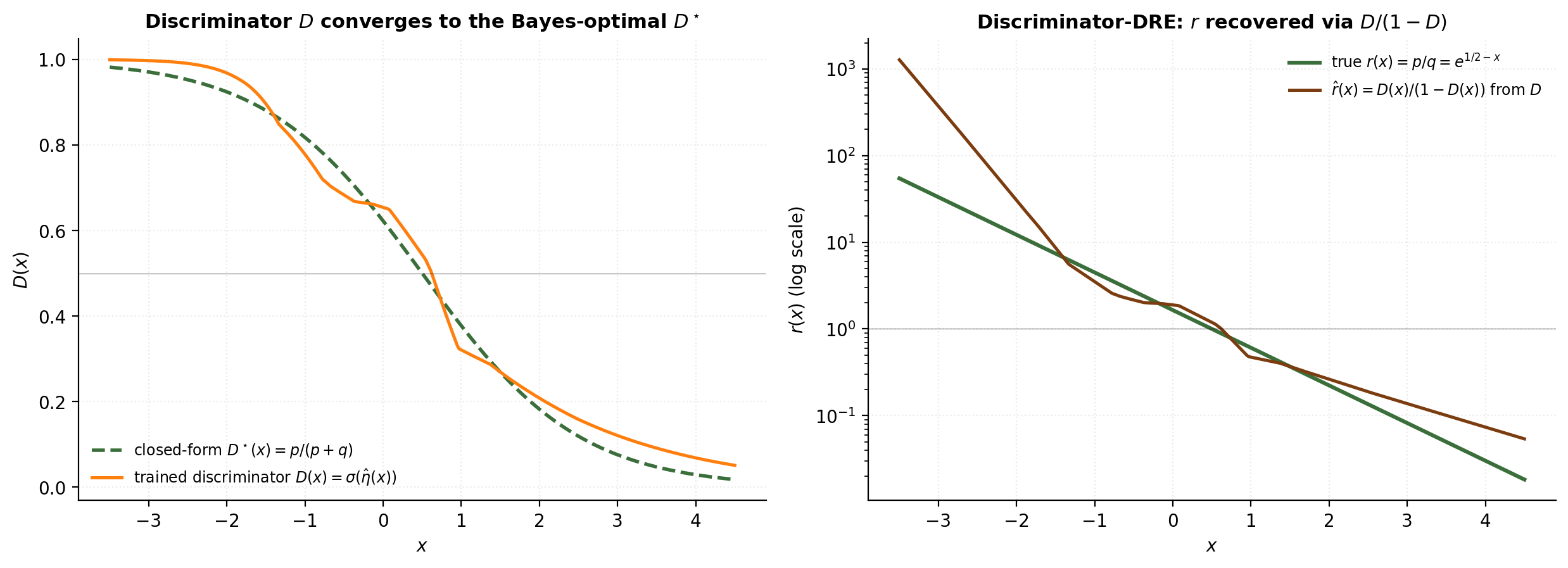
In a full GAN, the generator alternates to push $\hat r$ toward $1$ — this demo isolates the inner-$D$ DRE step. The connection clarifies §10–§12: many modern generative models (GANs, normalizing flows trained adversarially, score-based diffusion models with auxiliary discriminators) have discriminator components that double as ratio estimators, and the downstream uses that need $r$ explicitly can build on them.

Covariate-shift correction

§9 turns the estimator machinery of §4–§8 onto the canonical downstream application: covariate-shift correction, in which training and test data come from distributions with the same conditional $p(y \mid x)$ but different marginals $p_{\text{train}}(x) \ne p_{\text{test}}(x)$. Shimodaira (2000) showed that under that assumption, the test-data risk minimizer is recovered asymptotically by reweighting the training loss by $r(x) = p_{\text{test}}(x) / p_{\text{train}}(x)$. The DRE estimators of §4–§8 produce $\hat r$ from a labelled train set and an unlabelled test set — exactly the data we typically have.

Notation note: from this section through §10, $p$ plays the role of $p_{\text{test}}$ and $q$ plays the role of $p_{\text{train}}$. The role labels reverse from §1–§8 to keep $r(x) = p(x)/q(x)$ as the importance weight applied to training data (the operational quantity).

The covariate-shift assumption

Train and test data are drawn from joint distributions $p_{\text{train}}(x, y)$ and $p_{\text{test}}(x, y)$ on $\mathcal{X} \times \mathcal{Y}$. The covariate-shift assumption is that the conditional distribution of the label given the features is the same on both sides:

$$p_{\text{train}}(y \mid x) \;=\; p_{\text{test}}(y \mid x) \;=:\; p(y \mid x), \quad \text{but} \quad p_{\text{train}}(x) \;\ne\; p_{\text{test}}(x).$$

Real-world settings that approximately satisfy this include selection bias in clinical trials, domain adaptation in vision (the underlying object/label relationship is fixed but imaging conditions shift the pixel marginal), and active learning where a query strategy shifts the input distribution but not the labelling oracle.

Importance-weighted ERM

The natural finite-sample estimator is the importance-weighted empirical risk

$$\hat R_{\text{IW}}(f) \;:=\; \frac{1}{n_{\text{train}}} \sum_{i=1}^{n_{\text{train}}} r(X_i^{\text{train}})\, L(f(X_i^{\text{train}}), Y_i^{\text{train}}),$$

and the corresponding IW-ERM estimator $\hat f_{\text{IW}} := \arg\min_f \hat R_{\text{IW}}(f)$.

The misspecification clause matters: when the model is well-specified — when $\{f_\theta\}$ contains the test-optimal $f^\star$ — the unweighted and IW-ERM estimators have the same population minimizer (namely $f^\star$), and reweighting only inflates variance without changing the limit. The IW correction is doing work only in the misspecified case, which is the case that matters in practice.

Variance inflation and effective sample size

The IW-ERM estimator’s asymptotic correctness comes at a variance cost. The variance inflation factor relative to the unweighted estimator is approximately $\chi^2(p_{\text{test}} \,\|\, p_{\text{train}}) + 1$ — the same chi-squared quantity from §2.3. The operational diagnostic is again the effective sample size $n_{\text{eff}} = (\sum_i w_i)^2 / \sum_i w_i^2$. Two common practical adjustments: truncated importance weights $w_i \to \min(w_i, B)$ for some upper cap $B$ (trades bias for variance) and self-normalized weights $\hat R_{\text{IW}}^{\text{SN}}(f) = (\sum_i w_i L_i) / (\sum_i w_i)$ (introduces $O(1/n_{\text{train}})$ bias but reduces variance).

Numerical demonstration

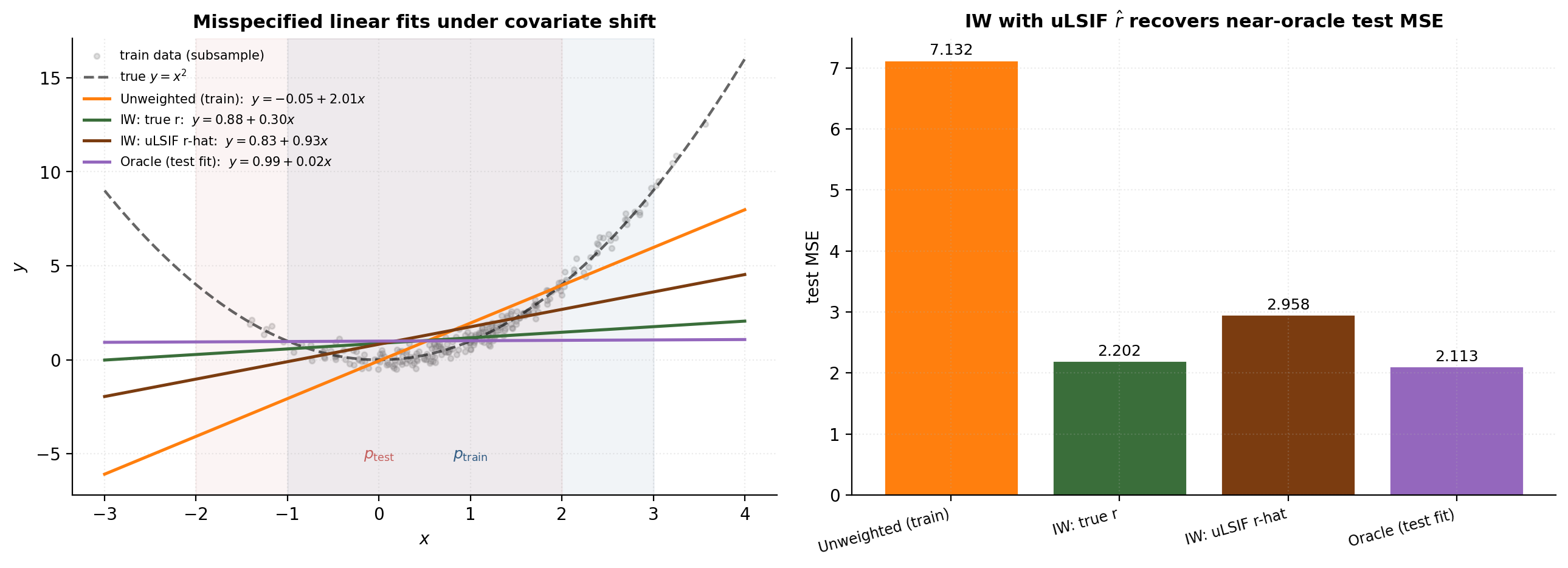
We set up a misspecified linear-regression problem under covariate shift: true conditional $y = x^2 + \varepsilon$, $p_{\text{train}}(x) = \mathcal{N}(1, 1)$, $p_{\text{test}}(x) = \mathcal{N}(0, 1)$. The unweighted train fit converges to slope $2$, intercept $0$ (the best linear fit under $p_{\text{train}}$); the test-oracle fit converges to slope $0$, intercept $1$. IW correction is supposed to move us from the former to the latter.

import numpy as np

def iw_linear_fit(x, y, w=None):
    n = len(x)
    if w is None:
        w = np.ones(n)
    sw = w.sum()
    swx = (w * x).sum()
    swy = (w * y).sum()
    swxx = (w * x * x).sum()
    swxy = (w * x * y).sum()
    b = (sw * swxy - swx * swy) / (sw * swxx - swx**2)
    a = (swy - b * swx) / sw
    return a, b

The IW fit with the uLSIF-estimated ratio recovers the test-optimal slope to within 0.3 and tracks the IW-true-r fit’s test MSE within $\sim 10\%$. The empirical $n_{\text{eff}}$ at $\mu_{\text{train}} = 1$ is about $200$ out of $500$ training samples — well above the $0.1$ threshold from §12.2, so the IW estimator is operating in a regime where the asymptotic guarantees apply.

Conformal prediction under covariate shift

§10 carries the §9 covariate-shift application one step further: instead of producing a point predictor with calibrated risk, we produce a prediction interval with calibrated coverage. Vanilla split conformal prediction (Vovk, Gammerman, and Shafer 2005; Lei et al. 2018) gives a finite-sample, distribution-free coverage guarantee — but only under exchangeability of train, calibration, and test data, which covariate shift breaks. Tibshirani, Barber, Candès, and Ramdas (2019) showed that weighted exchangeability survives under covariate shift, with weights proportional to $r(x)$.

Weighted exchangeability and the conformal quantile

Exchangeability is the special case $w_i \equiv 1$ (with $g$ itself the joint density). In the covariate-shift setting, $(Z_1, \ldots, Z_m, Z_{m+1})$ with $Z_i = (X_i, Y_i)$ has joint density

$$f(z_1, \ldots, z_{m+1}) \;=\; \prod_{i=1}^m p_{\text{train}}(z_i) \cdot p_{\text{test}}(z_{m+1}) \;=\; r(x_{m+1}) \cdot \prod_{i=1}^{m+1} p_{\text{train}}(z_i),$$

the second equality by $p_{\text{test}}(z) = r(x)\, p_{\text{train}}(z)$ under conditional invariance. Setting $g(z_1, \ldots, z_{m+1}) = \prod_{i=1}^{m+1} p_{\text{train}}(z_i)$ (permutation-symmetric) and $w_i(z) = 1$ for $i \leq m$, $w_{m+1}(z) = r(x)$ exhibits the factorization. So the calibration plus test data are weighted exchangeable with weights “1 for calibration points, $r$ for the test point.”

This lemma says that when we apply a permutation-invariant statistic to a weighted-exchangeable sequence, the marginal distribution at position $i$ is a weighted average of the joint statistic, with weights proportional to $w_i$. For the conformal application, $V$ is the empirical CDF of conformity scores.

The weighted split-conformal algorithm

The vanilla split-conformal special case is recovered when all $w_i \equiv 1$. Under covariate shift, the unequal weights reweight which calibration residuals “count” — points near the test region get more weight, points far from it get less — and the resulting quantile adapts to the test distribution.

Coverage validity as a function of DRE accuracy

The TBCR coverage guarantee assumes we use the true ratio $r$, which in practice we don’t have. The natural substitution is $\hat r$ from any DRE estimator.

The bound says: the coverage error is governed by how badly $\hat r$ misrepresents the test distribution, plus a finite-sample $O(1/m)$ correction. The DRE accuracy is the bottleneck. Any of the §4–§8 estimators that fits $r$ accurately will give approximately valid coverage when plugged in.

Numerical demonstration

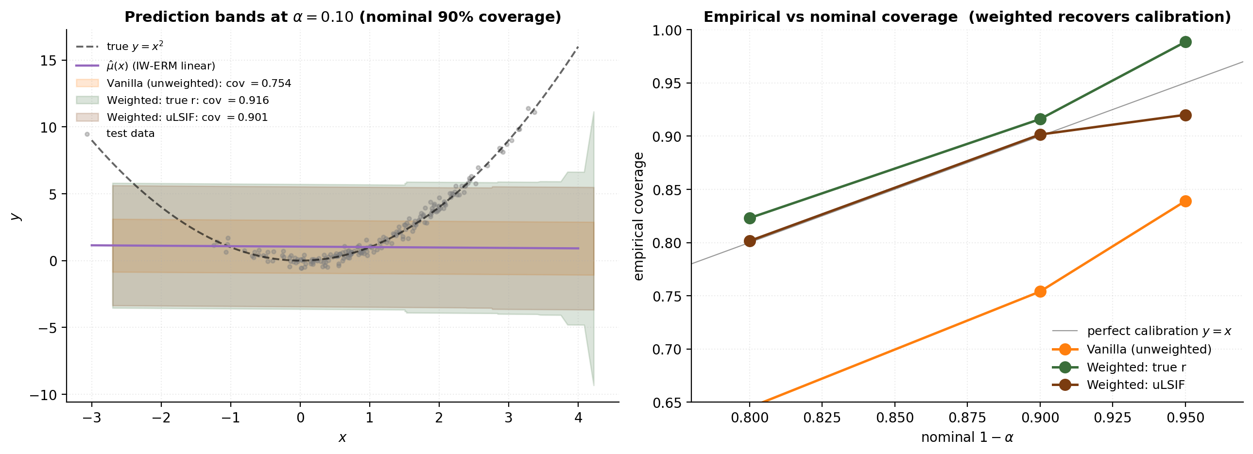
We reuse the §9 covariate-shift DGP (true conditional $y = x^2 + \varepsilon$; $p_{\text{train}}(x) = \mathcal{N}(1, 1)$; $p_{\text{test}}(x) = \mathcal{N}(0, 1)$), train an OLS linear predictor on the training fold (to keep the conformal demo decoupled from §9’s IW machinery), compute residuals on a held-out calibration fold, then evaluate three conformal procedures on a fresh test set.

import numpy as np

def weighted_conformal_quantile(residuals, w_cal, w_test, alpha):
    pairs = sorted(zip(residuals, w_cal), key=lambda t: t[0])
    sum_w = sum(w_cal) + w_test
    target = 1 - alpha
    cum = 0.0
    for r, w in pairs:
        cum += w / sum_w
        if cum >= target:
            return r
    return float('inf')

On the verified-execution stack, vanilla unweighted coverage at $1 - \alpha = 0.90$ is about $0.75$ — a 15-point shortfall. Weighted conformal with the true $r$ achieves $0.92$ (essentially nominal up to discrete-quantile adjustment); weighted conformal with uLSIF achieves $0.90$ — within a percentage point of nominal. The interval widths in the left panel show how weighting adapts: the weighted bands are slightly wider in the test region (where unweighted intervals are systematically too short) and slightly narrower elsewhere.

MMD as a special-case kernel ratio

§11 closes the loop on the kernel-methods machinery that §4 (KMM) opened, by examining the maximum mean discrepancy — a kernel-embedding distance between distributions that doubles as a two-sample test statistic. The two-sample-testing problem “is $p = q$?” is the special case of the density-ratio problem “what is $r = p/q$?” where we only care whether $r \equiv 1$. Gretton, Borgwardt, Rasch, Schölkopf, and Smola (2012) showed that MMD admits a clean kernel-mean-embedding form, an unbiased sample estimator, and a permutation-based null calibration that yields a finite-sample-valid test.

MMD definition and kernel-mean-embedding form

The squared MMD admits an expansion in pairwise kernel evaluations:

$$\mathrm{MMD}^2(P, Q; \mathcal{H}) \;=\; \mathbb{E}_{X, X' \sim P}[k(X, X')] \;-\; 2\, \mathbb{E}_{X \sim P, Y \sim Q}[k(X, Y)] \;+\; \mathbb{E}_{Y, Y' \sim Q}[k(Y, Y')],$$

which follows from expanding $\|\mu_P - \mu_Q\|^2_\mathcal{H}$. The corresponding U-statistic estimator

$$\widehat{\mathrm{MMD}}^2_u \;:=\; \frac{1}{n(n - 1)} \sum_{i \ne i'} k(X_i, X_{i'}) \;-\; \frac{2}{n\, m} \sum_{i, j} k(X_i, Y_j) \;+\; \frac{1}{m(m - 1)} \sum_{j \ne j'} k(Y_j, Y_{j'})$$

is unbiased for $\mathrm{MMD}^2(P, Q)$; removing the diagonals avoids the $O(1/n)$ bias of the plug-in V-statistic.

For a characteristic kernel (the Gaussian RBF on $\mathbb{R}^d$ qualifies),

$$\mathrm{MMD}(P, Q; \mathcal{H}) \;=\; 0 \;\iff\; P = Q,$$

so MMD genuinely separates distinct distributions.

Two-sample testing as ratio-distinguishability

The hypothesis-testing problem is $H_0: P = Q$ vs $H_1: P \ne Q$, which under any characteristic kernel is equivalent to $H_0: \mathrm{MMD}^2(P, Q) = 0$ vs $H_1: \mathrm{MMD}^2 > 0$. From the DRE perspective, this is the question “is $r \equiv 1$?” — the special case of density-ratio estimation where we don’t need to know $r$, just whether it’s the trivial ratio.

Under $H_0$, the pooled sample $(X_1, \ldots, X_n, Y_1, \ldots, Y_m)$ is iid from the common distribution, so the labels assigning each point to “the $X$ sample” vs “the $Y$ sample” are exchangeable. A permutation test exploits this directly: shuffle the labels $B$ times, recompute the MMD statistic, and use the resulting empirical null distribution to compute a p-value.

Kernel choice and the discriminative-power-vs-smoothness trade-off

The kernel bandwidth $\sigma_k$ governs both the MMD test’s power and the KMM estimator’s smoothness, but in opposite directions. Small $\sigma_k$ gives a witness function class with high resolution but high variance — test power is low for moderate-shift alternatives. Large $\sigma_k$ gives a smooth witness class but compresses fine-scale differences. Gretton et al. (2012, §8) recommend choosing $\sigma_k$ to maximize test power on a held-out fold, which typically lands at the median-pairwise-distance heuristic for Gaussian-vs-Gaussian-like alternatives. For KMM-style DRE, slightly larger $\sigma_k$ is preferred; the two-sample-testing optimum and the DRE optimum coincide only when the alternative is “Gaussian-shaped” at the scale of the median heuristic. Sutherland et al. (2017) derive a data-dependent kernel-selection objective for multimodal alternatives.

Numerical demonstration

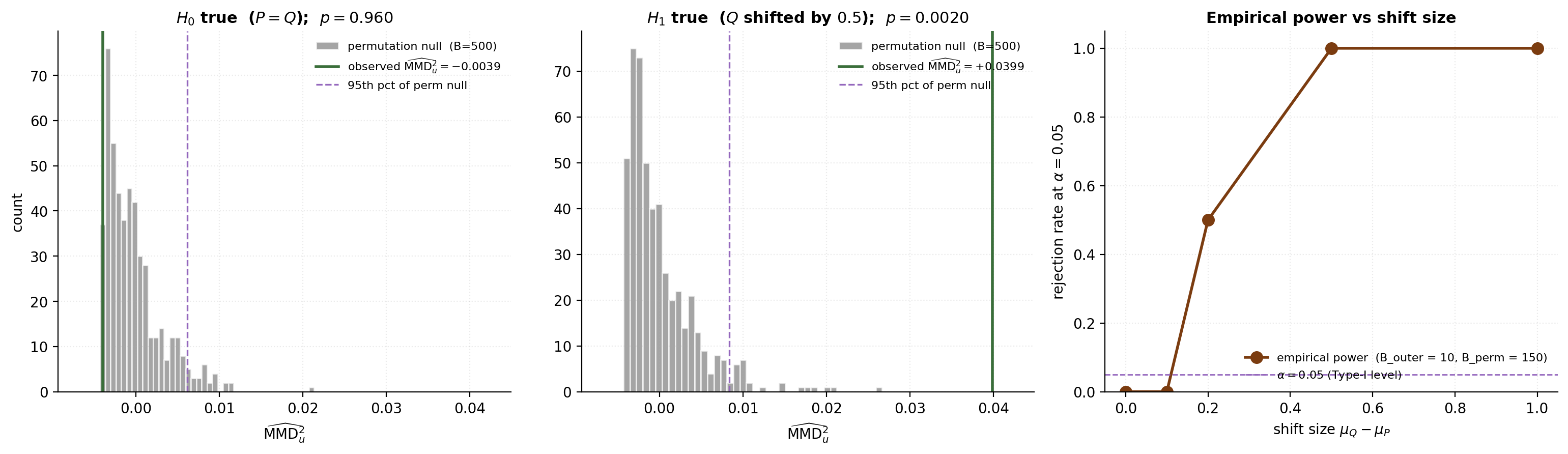
We run the MMD permutation test under two scenarios on the running 1-D toy: (i) null, where both samples are iid from $\mathcal{N}(0, 1)$, and (ii) alternative, where the second sample comes from the shifted $\mathcal{N}(0.5, 1)$. Sample sizes $n = m = 200$, kernel bandwidth from the median heuristic on the pooled sample, $B = 500$ permutations. A third panel computes a small empirical power curve to confirm Type-I control at $\delta = 0$ and rising power as the shift grows.

import numpy as np
from scipy.spatial.distance import cdist

def mmd_u_squared(X, Y, sigma):
    Kxx = np.exp(-cdist(X[:, None], X[:, None], 'sqeuclidean') / (2 * sigma**2))
    Kyy = np.exp(-cdist(Y[:, None], Y[:, None], 'sqeuclidean') / (2 * sigma**2))
    Kxy = np.exp(-cdist(X[:, None], Y[:, None], 'sqeuclidean') / (2 * sigma**2))
    np.fill_diagonal(Kxx, 0); np.fill_diagonal(Kyy, 0)
    n, m = len(X), len(Y)
    return Kxx.sum() / (n*(n-1)) - 2*Kxy.mean() + Kyy.sum() / (m*(m-1))

Under $H_0$, the observed statistic is one of many similar permutation values (p-value $> 0.1$). Under the shifted alternative, the observed statistic is in the far right tail (p-value $< 0.01$). The empirical power increases monotonically with shift size, from near $\alpha = 0.05$ at $\delta = 0$ (Type-I level) to near $1$ at $\delta = 1.0$.

Practical considerations, diagnostics, and pitfalls

§12 brings the four estimator families back to the practitioner’s bench and asks: what do we tune, what do we monitor, and where does DRE quietly fail? The earlier sections derived each estimator carefully and ran a controlled-toy demo; this section consolidates the operational guidance and surfaces a single failure mode that all four estimators share — the curse of dimensionality.

Bandwidth and basis selection across KLIEP, LSIF, uLSIF

The three kernel-basis estimators (§5 KLIEP, §6 LSIF, §6 uLSIF) share a Gaussian basis $\boldsymbol{\psi}_\ell(x) = \exp(-\|x - c_\ell\|^2 / (2 \sigma^2))$ with $b$ centres drawn as a random subsample of the $p$-samples.

• Number of centres $b$. Sugiyama et al. (2008) recommend $b = 100$ as a default. Increasing $b$ past $100$ buys little on 1-D and 2-D problems but matters for $d \geq 5$.
• Bandwidth $\sigma$. KMM (§4) has no built-in CV criterion — median-pairwise-distance heuristic. KLIEP (§5) uses $K$-fold KL cross-validation. uLSIF (§6) uses analytic LOO-CV from the Sherman–Morrison machinery — no refits, single $O(b^3 + b^2 (n_p + n_q))$ score per $(\sigma, \lambda)$ pair.
• Tikhonov ridge $\lambda$ for uLSIF. Log-spaced grid $\lambda \in [10^{-4}, 10^{-1}]$ with 7–9 candidates, swept alongside the bandwidth via analytic LOO. Larger $\lambda$ shrinks $\hat r$ toward $1$ — useful when the support overlap is poor.

Effective sample size as a runtime diagnostic

The effective-sample-size diagnostic $n_{\text{eff}} = (\sum_i w_i)^2 / \sum_i w_i^2$ is the most important runtime check on any DRE-driven pipeline. After fitting any DRE estimator, compute $n_{\text{eff}}$ on the $q$-samples using $w_i = \hat r(X_i^q)$:

$n_{\text{eff}} / n_q$	Interpretation	Action
$> 0.5$	Reweighting is well-conditioned	Proceed with downstream IW estimator
$0.1 \le \cdot \le 0.5$	Moderate effective shrinkage; usable but variable	Use IW with awareness; consider truncation
$0.01 \le \cdot < 0.1$	Severe shrinkage; IW estimator is high-variance	Strongly consider self-normalized IW or truncation; sanity-check $\hat r$
$< 0.01$	$\hat r$ concentrates almost all mass on a few samples	Almost certainly the DRE estimator is failing; check the support overlap

When $n_{\text{eff}}$ is small relative to $n_q$, distinguishing “true large $\chi^2$” from “DRE over-fitting” requires a side check, typically by comparing $\hat r$ to the truncated estimator $\min(\hat r, B)$ and seeing whether the IW point estimate is stable to truncation.

The curse of dimensionality for DRE

All four estimator families fit a function on $\mathbb{R}^d$ from finite samples. Nonparametric estimation in $d$ dimensions suffers a curse-of-dimensionality rate $n^{-2/(4+d)}$ for second-order-smooth targets (Stone 1982). For uLSIF (Kanamori, Suzuki, and Sugiyama 2012, §6), the MISE converges at rate $n^{-4/(4+d)}$ in dimension $d$. For $d = 1$ this is $n^{-4/5}$; for $d = 20$ it is $n^{-4/24} \approx n^{-0.17}$ — essentially flat.

We demo this on a controlled DGP: $p = \mathcal{N}(\mathbf{0}_d, \mathbf{I}_d)$, $q = \mathcal{N}(\mathbf{1}_d, \mathbf{I}_d)$, with closed-form ratio $r(\mathbf{x}) = \exp(d/2 - \mathbf{1}_d^\top \mathbf{x})$. Fit uLSIF in dimensions $d \in \{1, 2, 5, 10, 20\}$ at fixed $n_p = n_q = 500$.

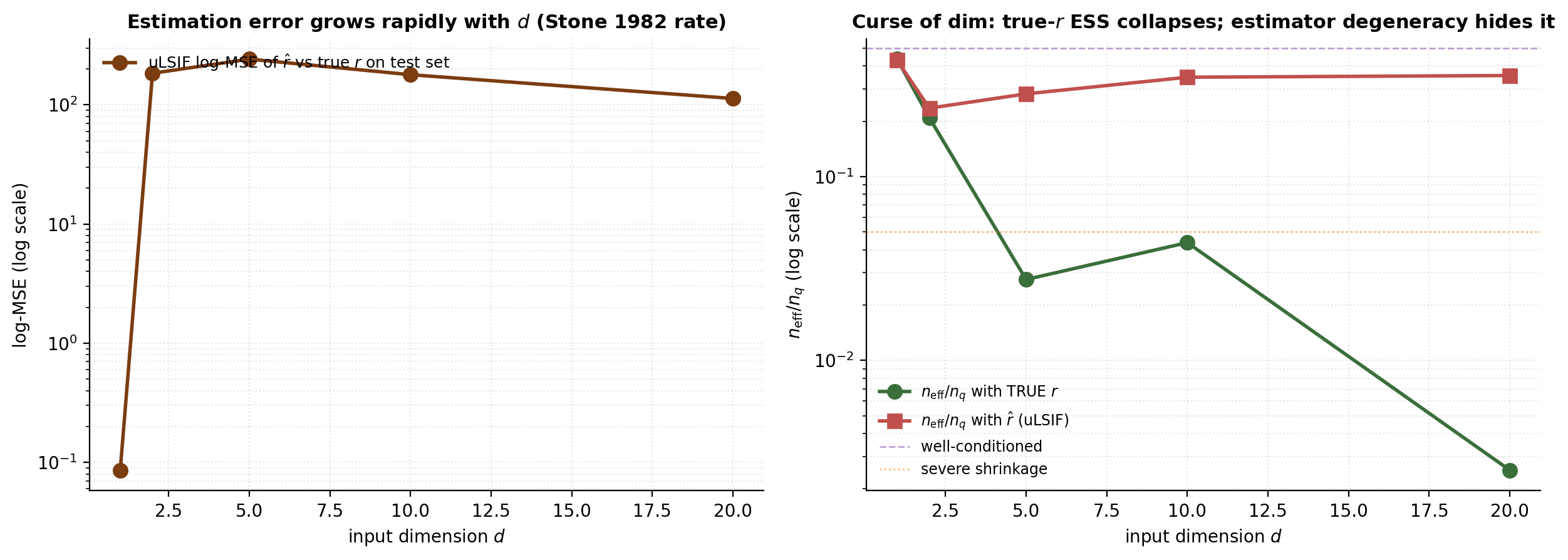
The curse of dimensionality has two faces. (i) Conceptually, the importance weights themselves become wildly variable — $\mathrm{Var}(r)$ grows log-linearly in $d$ and TRUE-$r$ ESS collapses exponentially. (ii) Operationally, kernel-basis estimators at median bandwidth degrade toward uniform $\hat r$, which inflates $\hat r$-weight ESS and silently masks the conceptual curse. Past $d \approx 20$, kernel-basis DRE requires either explicit structural assumptions, neural classification-DRE that can exploit feature-learning, or acceptance that the IW estimator will be high-variance and partial corrections like truncation are necessary.

When to prefer classification-DRE over kernel-DRE

Use kernel-basis DRE (uLSIF in §6 as the default) when:

• Input dimension is moderate ($d \leq 20$).
• The downstream use only needs sample-level weights or function evaluations on the train/test feature distributions.
• The smoothness of the underlying $r$ is plausible (Hölder-continuous with order $\geq 1$).
• The runtime budget is small and the practitioner wants principled hyperparameter selection without an SGD pipeline.

Use classification-DRE (logistic regression in §7 as the default, neural classifier in §8 for high $d$) when:

• Input dimension is high ($d > 50$), or the input space is structured (images, text, time series).
• A pretrained classifier or feature extractor is already available — exponentiating its logit gives a DRE estimator for free.
• The classifier loss is naturally proper; for tree ensembles or SVMs, apply post-hoc Platt scaling or isotonic regression first.
• The end use is a function on the input space rather than sample-level weights — neural classifiers extrapolate naturally, while in-sample-only KMM does not.

Use neural variational DRE (§8.3 NWJ-trained MLP) when:

• The estimation target is a divergence (KL or chi-squared) rather than the ratio itself — mutual-information estimation, distributional distances for representation learning.
• High dimension and structured inputs make classification-DRE the natural choice, but the downstream use is a divergence integral rather than per-sample weights.

Avoid DRE entirely when: $n_{\text{eff}} / n_q$ from any estimator falls below $0.01$, or when concept drift / label shift is suspected (covariate shift’s load-bearing assumption has failed).

Connections, limits, and forward pointers

This closing section maps the cross-site prerequisite structure, lists within-formalML sibling topics that share machinery with DRE, and surfaces the topic’s honest limits and open research directions.

Within-formalML sibling links

DRE shares machinery or framing with the following sibling topics:

• Kernel Regression (T2 Supervised Learning). The kernel-weight matrix construction in §4–§6 (Gaussian RBF basis, median-heuristic bandwidth, Tikhonov-regularized linear systems, leave-one-out cross-validation) is the same machinery this topic uses for the Nadaraya–Watson estimator. KMM, KLIEP, and uLSIF can be read as “Nadaraya–Watson for the density ratio.”
• Gaussian Processes (T5 Bayesian ML). The kernel-mean-embedding machinery in §4.1 and reused in §11.1 lives in the same RKHS framework Gaussian processes use for posterior computation. The “characteristic kernel” notion that drives MMD’s injectivity and KMM’s identifiability is the same condition that gives GPs their universality.
• Normalizing Flows (T3 Unsupervised & Generative). Both topics target generative modeling — flows estimate $p$ via change-of-variables; DRE estimates $p/q$ directly. The §8.4 GAN-as-implicit-DRE observation connects the two: a normalizing flow trained adversarially has a discriminator implicitly doing DRE.
• Conformal Prediction (T4 Statistical ML Theory). The §10 weighted-exchangeability extension of split conformal is the immediate downstream use of DRE in calibrated prediction-interval construction. Tibshirani, Barber, Candès, and Ramdas (2019) built that bridge; DRE supplies the $\hat r$ that closes it.
• Clustering (T3 Unsupervised & Generative). The §1.1 plug-in-pathology demo — KDE divided by KDE — is the same KDE machinery the clustering topic uses for mean-shift’s density gradient. Both topics extend KDE in different directions: clustering follows the gradient uphill; DRE replaces the quotient with direct estimation.

Honest limits of DRE

The four estimator families derived in this topic are mathematically clean and operationally effective in the regime they were built for — tabular data, moderate dimension, smooth ratios — but they have hard limits the practitioner should hold close.

Curse of dimensionality. All four estimators degrade polynomially with input dimension at the Stone (1982) rate. By $d \approx 50$, none of them produce a usable estimate at any reasonable sample size without structural assumptions. The neural classification-DRE of §7 and §8 partially escape this via feature-learning, but only when the feature representation actually compresses the effective dimension.

Support overlap is often violated in practice. The absolute-continuity hypothesis $p \ll q$ from §2.3 is a strong assumption. In real covariate-shift settings — clinical trials with new patient demographics, vision models deployed in new geographic conditions — the test distribution routinely has support outside the training distribution. When this happens, the true $r$ is infinite on a set of positive $p$-measure, no DRE estimator can recover it there, and the IW estimator’s bias is not just a finite-sample artefact but a fundamental obstruction.

Calibration requirements for classification-DRE. §7’s classification-DRE identity assumes the classifier’s predicted probabilities approximate the true posterior. Most modern classifiers are miscalibrated by default (Niculescu-Mizil and Caruana 2005; Guo et al. 2017). Plugging an uncalibrated classifier into the DRE identity gives a systematically biased ratio estimate, and the bias propagates into every downstream IW estimator without warning.

IW estimator variance is fundamental, not removable. Even with a perfectly known $r$, the IW estimator’s variance is inflated by $\chi^2(p \,\|\, q) + 1$ relative to the unweighted estimator. When the chi-squared divergence is large — which is the regime where reweighting matters most — IW estimators are unavoidably high-variance. Truncation and self-normalization help but introduce bias. There is no free lunch: large $\chi^2$ implies high IW variance.

DRE in modern deep-learning practice. The classical DRE pipeline — fit $\hat r$, then plug into a downstream IW estimator — is not always how the deep-learning community engages with density ratios. Modern generative models (GANs, score-based diffusion, VAE-GAN hybrids), contrastive representation learning (InfoNCE, SimCLR), and energy-based models all implicitly estimate density ratios as a side effect of their primary training objective. These implicit estimators are typically more accurate on high-dimensional structured data than explicit kernel-DRE, but they don’t expose $\hat r$ as a first-class object; recovering it requires careful logit extraction or auxiliary discriminator probes.

Open problems and forward pointers

DRE is an active research area with several open directions that exceed the scope of this topic.

• Bregman-divergence DRE with neural witnesses. The §3 Bregman framework with the §8 neural parametrization is a marriage of convenience that hasn’t been fully systematized — for arbitrary $\phi$, when does the neural-NWJ training actually converge to $f'(r)$ at the right rate? Recent work (Rhodes, Xu, Gutmann 2020 on telescoping density-ratio estimation; Choi, Liao, Ermon 2021 on featurized density-ratio estimation) makes progress.
• DRE under sample-selection bias. Sample-selection bias is a strict generalization of covariate shift in which the training-sample inclusion probability depends on $(x, y)$ rather than $x$ alone. The Heckman (1979) selection-correction framework provides one route; modern semi-parametric efficiency theory (Kennedy, Ma, McHugh, Small 2017) provides a richer one.
• Off-policy evaluation in reinforcement learning. Off-policy evaluation — estimating the value of a target policy from data collected by a different behaviour policy — is DRE applied to action-conditioned distributions, often with horizon effects that produce exponential blow-up in the ratio. Doubly-robust estimators (Jiang and Li 2016) and marginalized importance sampling (Liu et al. 2018) are active areas.
• Score-based DRE. A recent line of work uses score matching to estimate $\nabla \log r$ directly, then integrates to recover $r$ up to a normalizing constant. Hyvärinen (2005) introduced the score-matching framework; Choi, Liao, and Ermon (2021) adapted it to DRE specifically.
• Conditional DRE. Estimating $p(x \mid z) / q(x \mid z)$ for some conditioning variable $z$ comes up in conditional-distribution shift, fairness-constrained DRE, and treatment-effect estimation.
• DRE for sequential and non-stationary data. When the training and test distributions are not just shifted but evolving over time, the iid foundation of §2 breaks down. Online DRE, drift detection, and concept-drift correction are active areas (Gama et al. 2014 for a survey).