Representation Learning
Sufficient statistics, autoencoders, contrastive learning, and the simplex equiangular tight frame — the three-way convergence of classical sufficiency, supervised neural collapse, and InfoNCE-optimal self-supervised encoders to the same geometric object under progressively weaker information assumptions.
§1. What is a representation, and what makes one good?
“Representation learning” sounds like a technique, but it’s closer to a research program: take a high-dimensional, structured input — an image, a sentence, a sensor stream — and learn a map into a vector space where the geometry is useful for whatever comes next. Usefulness is the load-bearing word, and the rest of this topic is an inquiry into what it means and how to optimize for it without knowing the downstream task in advance.
We approach the question along three roads. The first, sufficiency, is the oldest: classical statistics already has a precise notion of a “lossless summary” of data, and modern representation learning is, in a soft sense, trying to learn one without parametric assumptions. The second, reconstruction, drives the autoencoder family — if a low-dimensional code can rebuild the input, it must have captured the input’s structure. The third, invariance, drives contrastive methods — if two views of the same object map close together while unrelated objects map far apart, the geometry has learned what the object is rather than how it looked on any given day. The same destination, three viewpoints; the topic ends by reconciling them.
§1.1 The folk definition
A representation is a map — typically with much smaller than the ambient input dimension and the parameters learned from data — together with three desiderata the map should satisfy:
-
Task-relevant signal is preserved. A downstream classifier or regressor built on should perform almost as well as one built on itself. We make this precise in §2 (via sufficiency) and §9 (via linear probing).
-
Nuisance variation is discarded. Two inputs that differ only in “irrelevant” ways — viewpoint, lighting, paraphrase, channel noise — should map to nearby codes. What counts as nuisance is task-dependent; §5 makes the nuisance group explicit through positive-pair construction.
-
The geometry is linearly probe-friendly. A linear classifier on should recover the task. This is a much stronger property than “any classifier on works” — it asks that the relevant information be laid out along directions rather than buried in nonlinear submanifolds. Why we want this is pragmatic: linear probes are cheap, calibrated, and reveal what the representation actually learned. §9.1 returns to this.
These three desiderata aren’t independent — preserving signal while discarding nuisance, in the limit, forces a linear geometry — but at the level of folk intuition they’re the three things practitioners check.
§1.2 A motivating vignette
To make the question “what makes a representation good?” concrete, we set up a synthetic fixture we’ll re-use in §3 and §12. Sample two classes in :
- Class means and , with . The discriminative direction is the first coordinate.
- A diagonal covariance with variance along the discriminative axis and almost everywhere else, but variance along the last coordinate — a high-variance nuisance direction uncorrelated with the class label.
Now project the cloud into three ways:
- Random: project onto two orthonormal random axes — the naive baseline.
- PCA: project onto the top two eigenvectors of the sample covariance.
- LDA: project onto Fisher’s linear-discriminant direction (1D) padded with one orthogonal axis — the supervised reference representation.
The figure shows what each projection sees. PCA’s top eigenvector is almost exactly , the nuisance axis — it found the direction of maximum variance, which is not the direction of maximum signal. LDA finds the discriminative direction because it uses the labels. A 5-NN classifier on each 2D projection makes the gap precise: random ≈ 0.55, PCA ≈ 0.81, LDA ≈ 0.82.
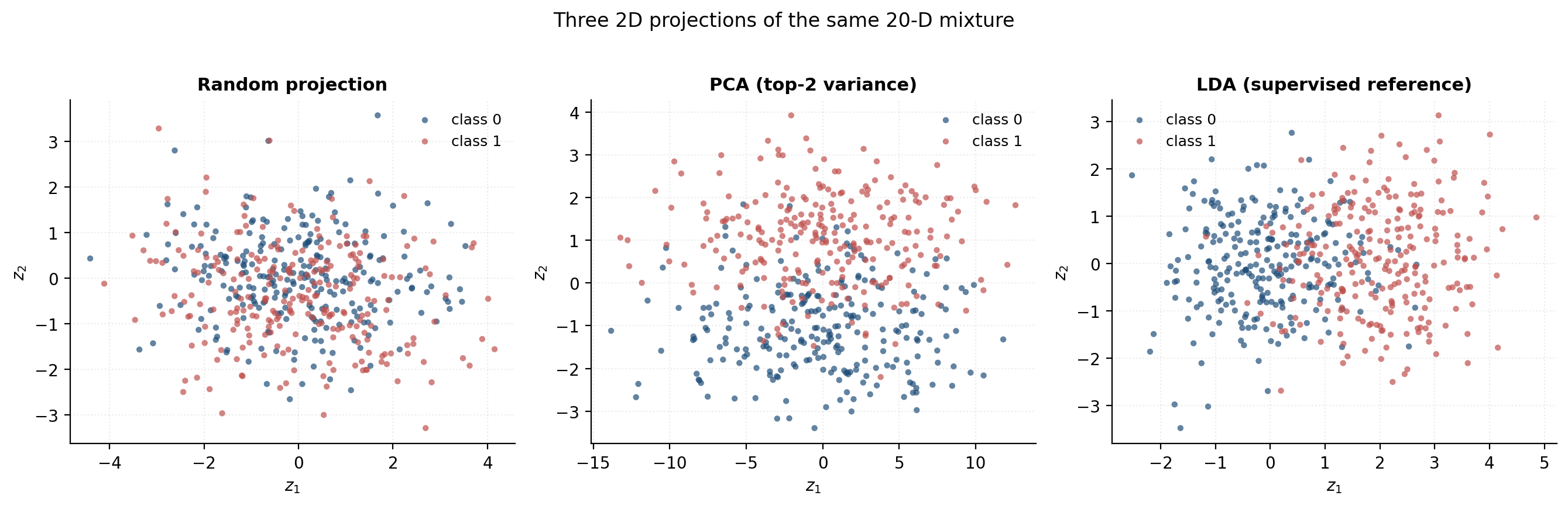
This is the central question of the topic: can we approximate the LDA-like projection without labels? The answer is “approximately yes, under structural assumptions on the data,” and the three lenses below are three flavors of those assumptions.
§1.3 Three theoretical lenses
The same goal — “preserve signal, discard nuisance” — admits three different formalizations, and most of representation-learning theory is some version of one of these:
The sufficiency lens (§2). A representation is sufficient for a task if the conditional distribution doesn’t actually depend on . The classical Fisher–Neyman factorization gives this a precise form; we relax it to “soft sufficiency” — keep — and ask which estimators achieve it. The autoencoder is the case (predict yourself); the contrastive critic is the case (predict the augmented view). The information bottleneck of §7 is the Lagrangian form of approximate sufficiency.
The reconstruction lens (§3, §4). A representation is good if there exists a decoder with . The intuition: if the code suffices to rebuild the input, it must encode the input’s manifold structure. This gives us PCA (linear, §3.2), autoencoders (nonlinear, §3.1), denoising autoencoders (which connect to score matching, §3.4), and variational autoencoders (which couple reconstruction to a probabilistic prior on , §4).
The invariance lens (§5, §6). A representation is good if two related inputs map close together and unrelated inputs map far apart. The positive-pair distribution encodes which transformations the representation should be invariant to — color jitter for an image classifier, back-translation for a sentence encoder, sub-sequence sampling for time series. The InfoNCE objective makes this precise as a variational lower bound on mutual information; SimCLR, MoCo, and BYOL are engineering instantiations.
These lenses are not three different theories of representation learning; they’re three windows onto the same object. §12 shows the windows meet — a sufficient statistic, a low-distortion reconstruction code, and the optimum of an InfoNCE loss converge to the same geometry in the cases where we can solve all three closed-form.
§1.4 Roadmap
The topic is structured as theory → method → critique → synthesis:
- §2–§4 set up the statistical view: sufficiency, autoencoders, VAEs.
- §5–§6 set up the contrastive view: InfoNCE, SimCLR, design space.
- §7–§8 set up two synthesis lenses: the information bottleneck (§7) and self-supervised pretext tasks beyond contrastive (§8).
- §9–§10 set up the evaluation machinery and the honest limits: linear probing, the Saunshi guarantee, the impossibility theorems for unsupervised disentanglement.
- §11–§12 set up the computational and geometric payoff: what gets hard at scale, and what the learned geometry looks like.
- §13 closes the loop with cross-site connections and forward pointers.
The Bengio–Courville–Vincent (2013) survey is the closest mid-density entry point in the literature; this topic adds the theory threads that have matured since 2013 — InfoNCE, alignment-uniformity, neural collapse, the disentanglement impossibility results — and weaves them into a single narrative.
§2. Sufficient statistics as the limit point of “good representation”
The phrase “good representation” begs the question — good for what? In classical statistics there’s a precise answer, due to Fisher: good for inference about a parametric model. A statistic is sufficient for a parameter if, once we know , the rest of the data tells us nothing additional about . Sufficiency is the original lossless-compression theorem of mathematical statistics, and modern representation learning can be read as the empirical search for a soft, task-implicit version of it.
This section makes the bridge explicit. We restate Fisher–Neyman (§2.1), characterize minimal sufficient statistics via Lehmann–Schefé (§2.2), relax classical sufficiency to a smooth, information-theoretic version that makes sense without a model (§2.3), and prove the Bayes-risk equivalence property that makes sufficiency the right target for representation learning (§2.4).
§2.1 Fisher–Neyman factorization
Let be a family of densities on (continuous or discrete; we’ll write integrals and let the discrete case follow by replacing the integral with a sum). Let be a measurable map. Call a statistic — any function of the data, summarizing it into a value .
Definition 2.1 (sufficient statistic).
is sufficient for if the conditional distribution does not depend on for any .
The intuition: once you’ve seen , the residual variation in is distributed the same way no matter what generated the data. There is no additional information in that helps you pin down .
Sufficiency is hard to check from the definition because it asks something about conditional distributions. The Fisher–Neyman theorem replaces the check with a factorization of the joint density:
Theorem 2.1 (Fisher–Neyman factorization).
is sufficient for if and only if the density factorizes as
for some non-negative measurable functions (which may depend on ) and (which does not).
Proof.
Both directions, in the discrete case.
() Suppose . Fix and condition:
The factors cancel, leaving an expression that depends only on and — no . So is sufficient.
() Suppose is sufficient, so doesn’t depend on . Call that conditional . Then
which is the desired factorization with .
The continuous-density case requires a Radon–Nikodym argument and a careful choice of conditional version (Halmos–Savage 1949); the conclusion is the same.
∎Examples we’ll reuse. For with known , the sample mean is sufficient for : the joint density factors as
For unknown and , the pair is sufficient. For an exponential-family model , the natural sufficient statistic is the exponential-family itself — and the autoencoder of §3 is, in a sense, an attempt to learn one when the family is unknown.
The representation-learning reading. A sufficient statistic is a hand-designed encoder that is lossless for inference under a known parametric family. The rest of this topic asks: what do we do when the family is unknown, or when “inference about ” is the wrong question and we want a representation good for many downstream tasks?
§2.2 Minimal sufficient statistics
Sufficiency alone doesn’t constrain how compressed is. For any sufficient , the pair with any auxiliary is also sufficient — you can pad with junk. The interesting object is the most-compressed sufficient statistic.
Definition 2.2 (minimal sufficient statistic).
A sufficient statistic is minimal if, for every other sufficient statistic , there exists a measurable function with almost surely.
In words: every sufficient statistic factors through the minimal one. The minimal sufficient statistic is the coarsest summary you can compute and still have lost no information for -inference.
The Lehmann–Schefé characterization tells us how to find it.
Theorem 2.2 (Lehmann–Schefé minimality).
Define the equivalence relation iff the likelihood ratio does not depend on . Then any statistic whose level sets coincide with the equivalence classes of is a minimal sufficient statistic.
Proof.
The level sets are exactly the sets on which the parameter “cannot tell points apart” — i.e., where the data is informationally equivalent. A sufficient statistic must be constant on every such set (otherwise it would distinguish two informationally-equivalent points, an asymmetry that wouldn’t survive the factorization). So any sufficient statistic’s level sets are unions of these equivalence classes, which means — whose level sets are the equivalence classes — is a coarsening of any other sufficient statistic, i.e., minimal. Bahadur (1954) gives the full measure-theoretic argument.
∎Why minimality matters for representation learning. Pure sufficiency lets us cheat by carrying the full input around: is trivially sufficient for any model. Minimality forces compression — it says throw away everything that doesn’t distinguish parameters. This is the unsupervised-analog of what representation learning wants: a code that’s just rich enough for the downstream task and no richer.
The catch, of course, is that “the downstream task” isn’t fixed. The classical theory assumes a single parameter to estimate; modern representation learning is in the multi-task regime where is replaced by a family of downstream tasks. §2.3 generalizes minimal sufficiency to handle this.
§2.3 Approximate (soft) sufficiency
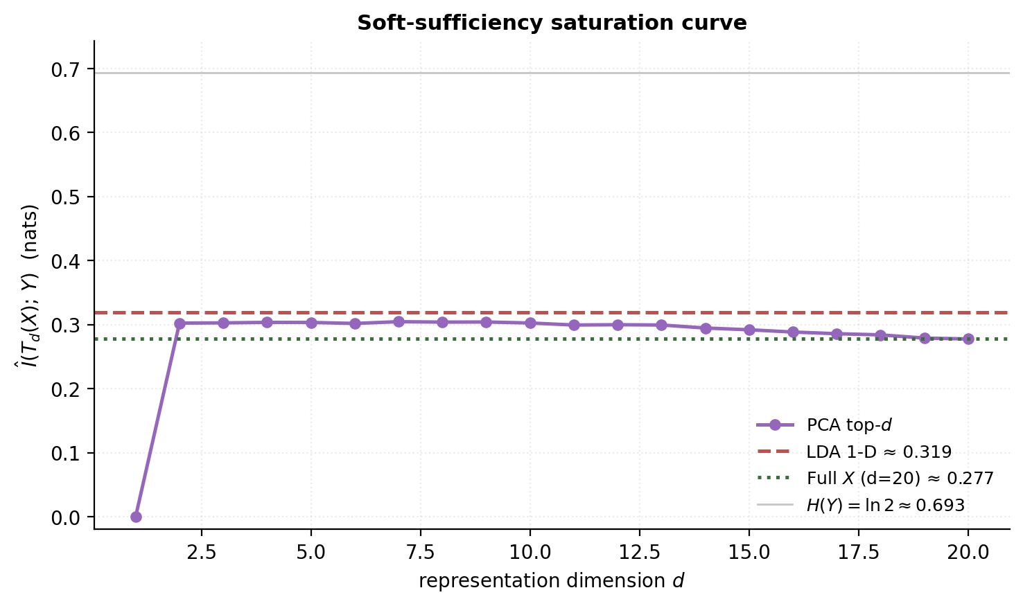
Classical sufficiency is binary: a statistic is or isn’t sufficient. For a learned representation , we want a smooth notion that lets us say “this representation is mostly sufficient.” The natural object is conditional mutual information.
Definition 2.3 (ε-sufficiency).
Given a downstream variable (a class label, a regression target, an augmented view), a representation is -sufficient for if
equivalently .
The equivalence is the chain rule for mutual information: , since is a function of and therefore .
When , the definition recovers a measure-theoretic version of classical sufficiency: is exactly sufficient for iff , which the chain rule gives as .
The bridge to representation learning. A learned encoder aims to minimize over a set of plausible downstream tasks. Three specializations recur throughout this topic:
- Supervised representation: is a known label and is trained to maximize directly. This is the supervised-learning setting; the IB theory of §7 gives the Lagrangian.
- Self-supervised representation: is replaced by an augmented view — same instance, different view. is trained to maximize . The InfoNCE bound of §5 gives a sample-computable lower bound on this MI.
- Generative representation: is the original input itself, viewed through a probabilistic decoder. The ELBO of §4 gives a sample-computable lower bound on , which is in turn related to by the data-processing inequality.
The three lenses of §1.3 are the three choices of .
A subtlety. involves entropies of high-dimensional continuous random variables, which are notoriously hard to estimate from samples. The InfoNCE bound of §5.3 is the workaround — instead of estimating , we maximize a lower bound that is sample-computable. The looseness of that bound is what separates representation-learning theory from the information-theoretic ideal of §2.3.
§2.4 Bayes-risk equivalence
Sufficiency has a striking decision-theoretic consequence: a sufficient statistic preserves the Bayes-optimal performance of any decision rule.
Theorem 2.3 (Bayes-risk equivalence under sufficiency).
Let be sufficient for , let be any loss function over actions , and let be the Bayes-optimal decision rule given a prior . Then there exists a decision rule with the same Bayes risk: .
Proof.
Define , the Bayes-optimal action given only the summary . We show this matches the full-data Bayes risk by the tower property. For any decision rule ,
The inner conditional expectation, by sufficiency, satisfies , so the conditional distribution of given doesn’t carry extra -information. Therefore the Bayes-optimal action given — call it — achieves the same conditional risk as the Bayes-optimal action given the full , and the outer expectation matches.
∎The corollary for representation learning. A sufficient statistic is a lossless representation for any decision problem in ‘s family. In the soft / multi-task version of §2.3, an -sufficient representation is approximately lossless for any task in the family — up to an additive slack in the Bayes risk, by Pinsker-type arguments we’ll formalize in §9.4 (Saunshi guarantee).
This is the mathematical target of representation learning: build such that downstream Bayes risks under are close to the Bayes risks under , without having access to the downstream tasks at training time. The rest of the topic gives constructive ways to do this — by reconstruction (§3, §4), by invariance (§5, §6), and by an explicit information-theoretic Lagrangian (§7).
§3. The autoencoder family
The reconstruction lens is the oldest unsupervised representation-learning principle in deep learning: if a low-dimensional code can rebuild the input, the code must have captured the input’s structure. The autoencoder makes this operational — pair an encoder with a decoder , train the composition to be the identity on the data, take whatever learned as the representation.
What makes the family interesting (and worth a section) is not the recipe but its theoretical content. The linear case is exactly PCA — Baldi–Hornik (1989) — which gives us a closed-form characterization of what the bottleneck recovers and a sharp lower bound on the reconstruction error in terms of the spectrum of the data covariance. The denoising variant of Vincent (2008) turns out to be implicitly estimating the score of the data distribution via the Tweedie identity. The sparse variant connects to classical dictionary learning. The VAE of §4 will quantize this whole picture with a probabilistic prior on the code; everything in this section is its deterministic ancestor.
§3.1 Definition
Definition 3.1 (autoencoder).
An autoencoder consists of two parametric maps,
jointly trained to minimize the reconstruction loss
The representation is the encoder output ; the bottleneck dimension is a hyperparameter, typically .
Three design choices distinguish AE variants. The function class — linear, shallow MLP, deep MLP, convolutional, transformer — controls expressivity. The reconstruction loss — squared error, cross-entropy for discrete inputs, perceptual losses for images — controls what “rebuild” means. The regularization on the encoder or the latents — denoising, sparsity, KL to a prior — controls what kind of code we incentivize. We work through these in order of theoretical content.
§3.2 Linear autoencoders are PCA
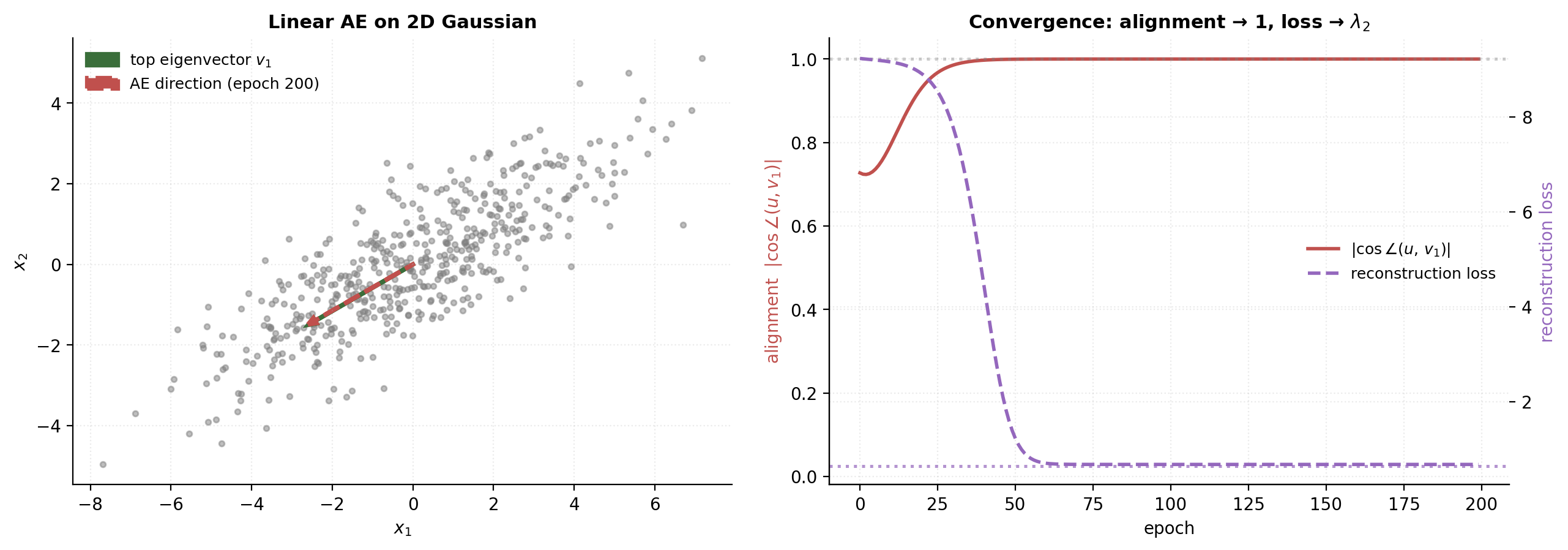
The simplest AE has linear encoder with and linear decoder with . Take mean-centered with covariance of full rank . The reconstruction loss becomes
Theorem 3.1 (Baldi–Hornik 1989).
The minimum of is achieved when equals the orthogonal projector onto the top- eigenspace of . The minimum value is
where are the eigenvalues of . The individual and are determined only up to an invertible reparametrization , for .
Proof.
We optimize first, holding fixed. The loss is quadratic in ; differentiating and setting the gradient to zero gives
so (assuming is invertible, which holds when has full row rank and is positive definite). Substituting back,
Make the change of variables . Then and , so the second trace becomes
where is the orthogonal projector onto the row space of — a rank- orthogonal projector in .
We are therefore maximizing over rank- orthogonal projectors . By Ky Fan’s maximum principle, this trace is maximized by the projector onto the top- eigenspace of , with maximum . So
The optimal has with row space spanning the top- eigenvectors of — equivalently, where stacks the top- eigenvectors and is any invertible matrix. The corresponding gives the product , the projector onto the top- eigenspace.
∎Reparametrization invariance. The product is identified; the individual and are not. Linear autoencoders therefore can’t learn “unique principal components” — they learn a rotated basis within the correct subspace. This is benign but worth knowing when interpreting the encoder weights of a trained AE.
The geometric reading. A linear AE projects the data onto the subspace of maximum variance and discards the orthogonal complement. The recovered subspace is identical to PCA’s. So PCA isn’t a competitor of representation learning — it’s the base case the rest of the topic generalizes.
§3.3 The bottleneck inequality and the manifold gap
Corollary 3.1 (bottleneck inequality).
For any linear autoencoder with bottleneck dimension trained on data with covariance of eigenvalues ,
with equality when is the top- eigenprojector.
This bound is a hard floor: no choice of linear can do better. The data “want” dimensions exactly when the spectrum of has a clean knee at index — i.e., the bottom eigenvalues sum to something small. When the spectrum is flat, no linear AE compresses well.
Where nonlinearity helps. The bottleneck inequality is linear-AE specific. Consider a data distribution supported on a smooth -dimensional submanifold of — say, points on a circle in (, ). The covariance has rank 2 in this case; the linear bottleneck floor is positive. But a nonlinear AE with even modest capacity can parametrize the circle by an angle and reconstruct it exactly, achieving at . The nonlinear AE is off-graph with respect to the linear-AE floor.
Where nonlinearity doesn’t help as much as you’d think. In practice, deep AEs on natural data (images, text embeddings) underperform their theoretical nonlinear ceiling because (a) the manifold hypothesis is approximate, not exact — there’s always noise off the manifold; (b) optimization is hard; (c) the squared-error loss is geometrically inappropriate for many natural data types. The VAE of §4 fixes (c) by switching from a deterministic squared-error decoder to a probabilistic one; §10’s identifiability theorems give us a vocabulary for talking about (a).
§3.4 Denoising autoencoders and the score-matching connection
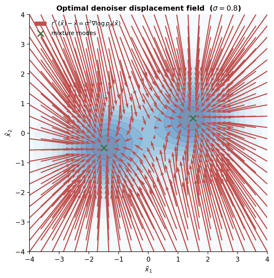
A denoising autoencoder corrupts the input with noise and trains the network to reconstruct the clean input from the corrupted version (Vincent 2008). Concretely, with Gaussian noise ,
This is the deterministic AE of §3.1 with a stochastic encoder input. The trick is that the population minimizer has a strikingly clean form, and that form connects denoising to score estimation.
Theorem 3.2 (Tweedie's identity / Vincent 2008).
Let and with independent of . Let denote the density of (the convolution ). Then the optimal denoiser satisfies
Proof.
By Bayes’ rule, , where is the density. The key gradient identity is
Differentiate the convolution under the integral sign:
The remaining integral is , so dividing through by gives
which rearranges to the claim.
∎The interpretation. The denoising displacement is the score of the smoothed density, scaled by . The DAE doesn’t just learn to clean inputs; it implicitly learns the gradient of the log-density in the neighborhood of the data manifold. This is the connection that diffusion models exploit in earnest: training a sequence of denoisers at different noise scales is training a sequence of score estimators, and the reverse-time SDE for sampling is built directly on those scores. Diffusion sits downstream of this topic — we’ll point at it from §13 — but the mathematical content of Tweedie is right here, three lines from the AE loss.
§3.5 Sparse autoencoders and dictionary learning
A sparse autoencoder adds a penalty on the latent activations to incentivize codes where only a small fraction of latent units fire for any given input (Olshausen–Field 1996, Ng 2011). The standard variants are
with two common choices of : the penalty (the Lasso of representation learning), or the KL penalty where is a target average activation rate (typically ) and is the empirical mean activation of the -th latent unit.
Why we’d want sparsity. With an overcomplete latent (), the AE without regularization has trivial perfect-reconstruction solutions (set ). Sparsity breaks this degeneracy by forcing the network to use a combinatorial code — different inputs activate different sparse subsets of the latents — which mirrors the sparse-coding model of biological vision (Olshausen–Field 1996) and makes the learned features more interpretable.
Dictionary-learning equivalence. The sparse-AE objective with linear decoder and penalty, , is exactly the dictionary-learning problem (Mairal et al. 2009): find an overcomplete basis and sparse codes that linearly reconstruct the data. The “encoder” is implicit — solving the lasso per input — but morally this is just a sparse AE where the encoder is replaced by an optimization solver. Modern sparse-AE work on transformer features (Bricken et al. 2023, Cunningham et al. 2023) is dictionary learning at scale with a learned (rather than optimization-based) encoder.
This closes the deterministic-AE family. The VAE of §4 replaces the deterministic squared-error decoder with a probabilistic one and the deterministic encoder with a variational posterior; the contrastive methods of §5 drop the decoder entirely in favor of an invariance signal. Both trajectories begin here.
§4. The variational autoencoder
The deterministic autoencoder of §3 has no story about uncertainty in the code. Given an input , the encoder returns a single point ; given a code , the decoder returns a single reconstruction . This works if the data lies cleanly on a low-dim manifold, but it makes the AE unhappy in two ways: there’s no principled way to sample new data, and there’s no way to express the encoder’s confidence about an ambiguous input.
The variational autoencoder (Kingma–Welling 2014; Rezende–Mohamed–Wierstra 2014) fixes both at once by replacing the deterministic encoder/decoder pair with a probabilistic latent-variable model. The training objective — the Evidence Lower Bound — is identical in form to the ELBO of variational inference, and three new pieces make it work end-to-end: the amortization of as a neural network, the reparametrization trick that lets gradients pass through the latent sampling step, and the closed-form Gaussian KL that makes the KL term trivially differentiable. We derive each in turn.
§4.1 A latent-variable generative model
Definition 4.1 (deep latent-variable model).
A deep latent-variable model is a triple where:
- is a fixed prior on (typically );
- is a parametric conditional density on , with parameters realized as a neural-network mapping ;
- the implied marginal density on is .
The model is generative because the prior-decoder pair defines a sampler: draw , then . Standard choices for are for continuous data (giving a squared-error reconstruction loss) and Bernoulli per pixel for binary data (giving a cross-entropy reconstruction loss). We’ll use the Gaussian decoder throughout because it makes the §3 connection transparent.
The training goal is maximum-likelihood estimation of :
This is what the AE of §3 isn’t doing — the deterministic AE optimizes reconstruction without any reference to a probability density. The VAE makes the connection explicit, but at the cost of an intractable integral: has no closed form when comes from a neural network. The ELBO is the workaround.
§4.2 The Evidence Lower Bound
The classical move (Jordan, Ghahramani, Jaakkola, Saul 1999) is to introduce an auxiliary density — call it a variational distribution — and use it to construct a lower bound on . The cleanest derivation is through a direct identity.
Theorem 4.1 (ELBO identity).
For any density on with wherever , and any ,
Proof.
Write the joint as and expand the ELBO:
where we used that doesn’t depend on to pull it out of the expectation. Rearranging gives the identity.
∎Corollary 4.1 (variational lower bound).
Since ,
with equality if and only if almost everywhere.
The ELBO is therefore a tight lower bound on — tight when is the true posterior — and at any it has the same gradient with respect to as would, up to the variational gap. We maximize the ELBO instead of the intractable , jointly over and the parameters of .
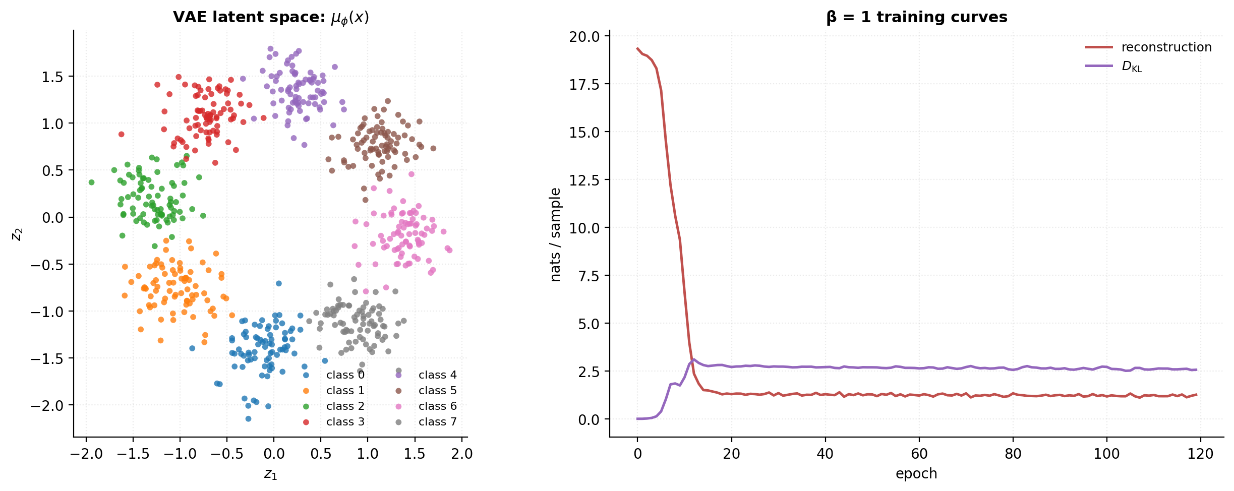
Amortization. Optimizing a separate for each data point scales linearly in dataset size and is impractical. The VAE amortizes the variational distribution by parametrizing as a neural network with shared parameters — a single encoder produces the variational distribution for every input. Common choice: , a diagonal Gaussian whose mean and (log-)variance are network outputs. The ELBO becomes
and we maximize this jointly over — encoder and decoder trained together by stochastic gradient ascent on the dataset average.
§4.3 Reconstruction + KL decomposition
The ELBO admits a particularly useful rewriting that exposes the two forces inside it.
Proposition 4.1 (ELBO decomposition).
For any latent-variable model,
Proof.
Substitute the joint factorization :
∎The geometric reading. Maximizing the ELBO pushes two objectives against each other:
- Reconstruction wants the decoder’s predicted distribution to put high probability on the actual input . For a Gaussian decoder with fixed variance, — the squared-error reconstruction loss of §3 wrapped in an expectation over .
- Regularization wants the encoder’s posterior to stay close to the prior . This is the new piece — it didn’t exist in the deterministic AE — and it’s what makes the VAE’s latent space samplable.
Why the KL term has a closed form. For Gaussian and Gaussian prior ,
This is a hand-derivable Gaussian-vs-Gaussian KL; no Monte Carlo needed. The reconstruction term, by contrast, does require Monte Carlo — which is what §4.4 enables to backpropagate through.
§4.4 The reparametrization trick
The gradient has a subtlety: the encoder parameters appear inside the distribution we’re integrating against, not just inside the integrand. The naive approach — sample , then differentiate — doesn’t work because the sampling step is not differentiable in .
Two estimators handle this:
Score-function estimator (REINFORCE). Use the log-derivative trick, , to write
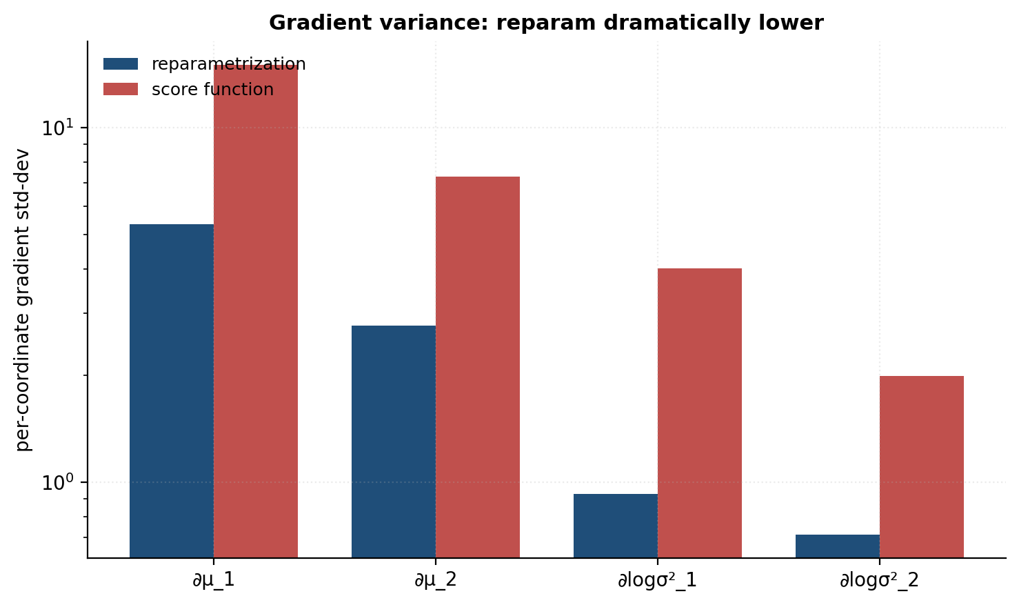
This is unbiased and works for any — including discrete distributions — but it’s notoriously high-variance because is not mean-zero in . The estimator is dominated by the magnitude of even when only its shape matters for the gradient.
Reparametrization estimator (Kingma–Welling 2014). If we can write the sample as a deterministic function of a noise variable that doesn’t depend on ,
then the gradient passes through:
For the diagonal Gaussian , the reparametrization is
The encoder outputs — both fully differentiable in — and the noise is fixed at sample time, breaking the non-differentiability.
Why the variance reduction. The reparametrization estimator uses the pathwise derivative — gradient flows through via — and exploits local smoothness of . The score-function estimator uses only the value of , treating it as a black box. When is smooth (as in VAE losses with neural decoders), pathwise gradients have dramatically lower variance. Empirically, the gap is one to three orders of magnitude on standard VAE benchmarks.
§4.5 Posterior collapse, β-VAE, and the rate-distortion view
In practice, training a VAE on data with a powerful decoder (e.g., a deep autoregressive ) reveals an unwanted failure mode: collapses to the prior , , and the encoder stops conveying information about . The latent space becomes useless and reconstruction relies entirely on the decoder’s unconditional capacity. This is posterior collapse, and it’s the VAE’s analog of the bottleneck-too-loose pathology.
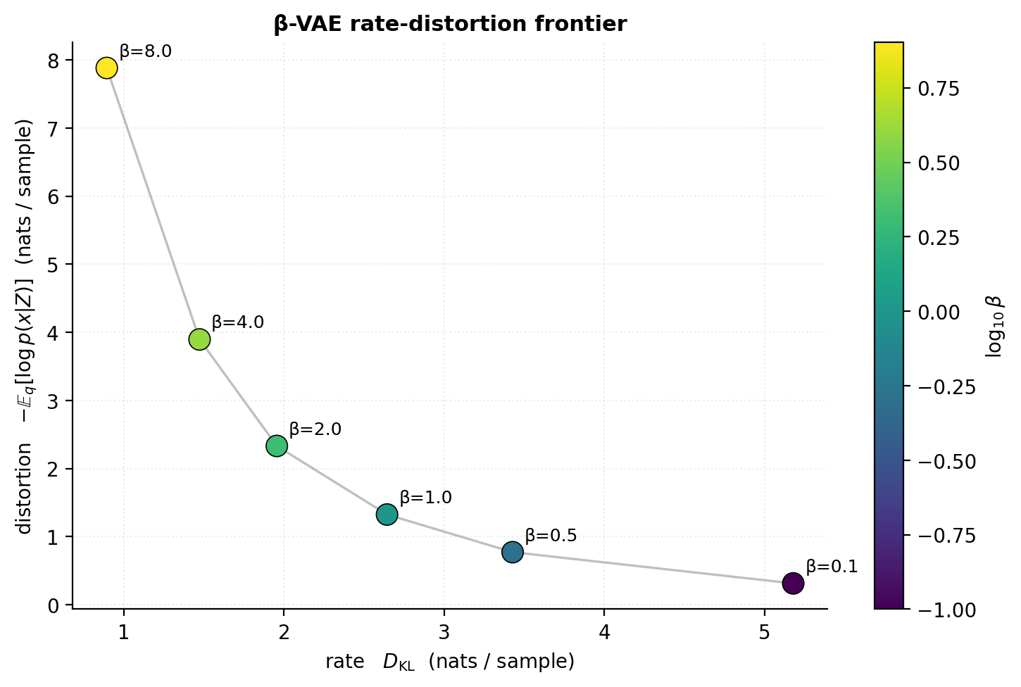
The β-VAE. Higgins et al. (2017) introduced a single-scalar generalization of the ELBO that lets us trade off reconstruction against KL deliberately:
At this is the standard ELBO. At , the KL penalty dominates and the encoder is incentivized to discard information — eventually collapsing to the prior. At , the KL penalty weakens and the encoder is free to encode more about each input, at the cost of a latent space that’s less prior-like (and less generatively useful).
The rate-distortion reading. The two terms are exactly the information-theoretic rate and distortion of the encoding:
- upper-bounds averaged over the data distribution (Alemi et al. 2018). This is the rate — bits per sample required to describe given the prior.
- is the distortion — average squared error (for Gaussian decoders) or cross-entropy (for Bernoulli decoders) between and its reconstruction.
Sweeping traces the rate-distortion frontier for this specific encoder / decoder pair. The full rate-distortion theorem gives the information-theoretic lower bound any such pair must respect; the β-VAE’s trade-off curve lies above it, with the gap measuring how “inefficient” the encoder/decoder are relative to the optimal vector quantizer.
This closes the variational autoencoder. The reconstruction lens has been formalized probabilistically; the next two sections shift to the invariance lens (§5 InfoNCE, §6 SimCLR), and §7 returns to this rate-distortion view under the explicit information-bottleneck objective.
§5. The contrastive principle and the InfoNCE bound
The reconstruction lens of §3-§4 asks the encoder to preserve enough of to rebuild it. The invariance lens asks something subtly different: preserve enough of to recognize — meaning the encoder should map two related views of the same instance close together and unrelated instances far apart. Two views of the same image (a crop, a color jitter), two paraphrases of the same sentence, two consecutive frames of the same video — these are the “positive pairs” the encoder should align. Everything else is, by default, a negative.
This section formalizes the invariance lens through the InfoNCE objective (Oord, Li, and Vinyals 2018), the closed-form connection to mutual-information estimation, and the alignment-uniformity decomposition of Wang and Isola (2020). The §5.4 detour explains why the contrastive critic at optimum is the log density-ratio of formalML’s density-ratio-estimation topic — the same object, in a different costume.
§5.1 Positive pairs and negative samples
The contrastive setup begins with a positive-pair distribution on . By construction, the marginals of are equal: , the data distribution. The “positivity” enters through correlation between and — they’re not independent samples but two related views of the same underlying instance.
Three canonical constructions:
- Augmentation-based positives. Define a stochastic augmentation (random crop, color jitter, dropout, back-translation, time-warp). Set — both and are independent augmentations of a shared anchor .
- Temporal positives. For sequential data, set — consecutive frames or tokens. This is the Oord et al. (2018) “contrastive predictive coding” setup.
- Multi-modal positives. are paired observations from two modalities (image, caption). The CLIP construction; we revisit in §8.
Negatives are typically implicit: given a batch of positive pairs, the negatives for anchor are the other batch members’ positives . Because is drawn from independently of , this gives valid negatives essentially for free — no separate negative-sampling step.
The augmentation group is the invariance prior. What the encoder is allowed to throw away is determined by the augmentation: anything two augmented views can differ on is, by construction, deemed irrelevant. Choosing the augmentation set is the unsupervised counterpart of choosing the label space.
§5.2 The InfoNCE objective
We parametrize an encoder (often with its output -normalized to the unit sphere, ) and define a similarity between two encoded views:
Here is the temperature, a scalar that controls how sharp the softmax becomes. Small makes the model pickier (only very-aligned pairs count as positive); large smooths the loss landscape.
Definition 5.1 (InfoNCE loss, batch form).
Given a batch of positive pairs and a critic , the InfoNCE loss is
When , the loss depends on the encoder parameters through the cosine similarity.
The inner expression is the categorical cross-entropy of the K-way classification problem “which in the batch is the positive partner of ?” — with the softmax temperature absorbed into the critic. A perfect encoder makes the diagonal of the similarity matrix high and the off-diagonal entries low; the loss penalizes deviations from that pattern.
Two variants you will encounter in the wild. (i) The “all-pairs” version treats every other batch element (both anchors and positives) as a candidate negative, giving negatives per anchor instead of — this is the NT-Xent loss of SimCLR (Chen et al. 2020) and is what we’ll use in §6. (ii) The “asymmetric” version uses separate encoders for the two views (MoCo’s “query” and “key” encoders) and a queue of cached negatives. These are engineering variants of the same underlying objective.
§5.3 InfoNCE as a variational lower bound on mutual information
The reason InfoNCE is interesting theoretically (and not just empirically) is that its negative is a tractable lower bound on the mutual information between the two views.
Theorem 5.1 (InfoNCE MI bound (van den Oord, Li, Vinyals 2018, Poole et al. 2019)).
For any positive-pair distribution with marginal , any critic , and any batch size ,
with equality (asymptotically in ) when for any function .
Proof.
We give the proof through the optimal-critic argument. Frame the problem as a -way classification: nature draws an index , then samples and a batch of candidates with (the positive is at index ) and independently for (the negatives are marginal samples). Given the observed , the goal is to recover .
Step 1: identify the Bayes-optimal critic. By Bayes’ rule,
where the second equality divides numerator and denominator by . The right side is the softmax of , the log density-ratio. Therefore is the Bayes-optimal classifier.
Step 2: compute the loss at . The InfoNCE loss is the categorical cross-entropy of identifying . At the Bayes-optimal classifier, the cross-entropy equals the conditional entropy:
Step 3: relate the conditional entropy to mutual information. By the identity , and using (uniform on classes),
Step 4: bound by . Under the generative model, is independent of marginally, so and . The information about contained in the batch given is at most the information shares with the positive — formally, by the chain rule and data-processing inequality:
Step 5: conclude. Combining steps 2-4,
For any other critic , Bayes-optimality gives , so the bound holds for arbitrary .
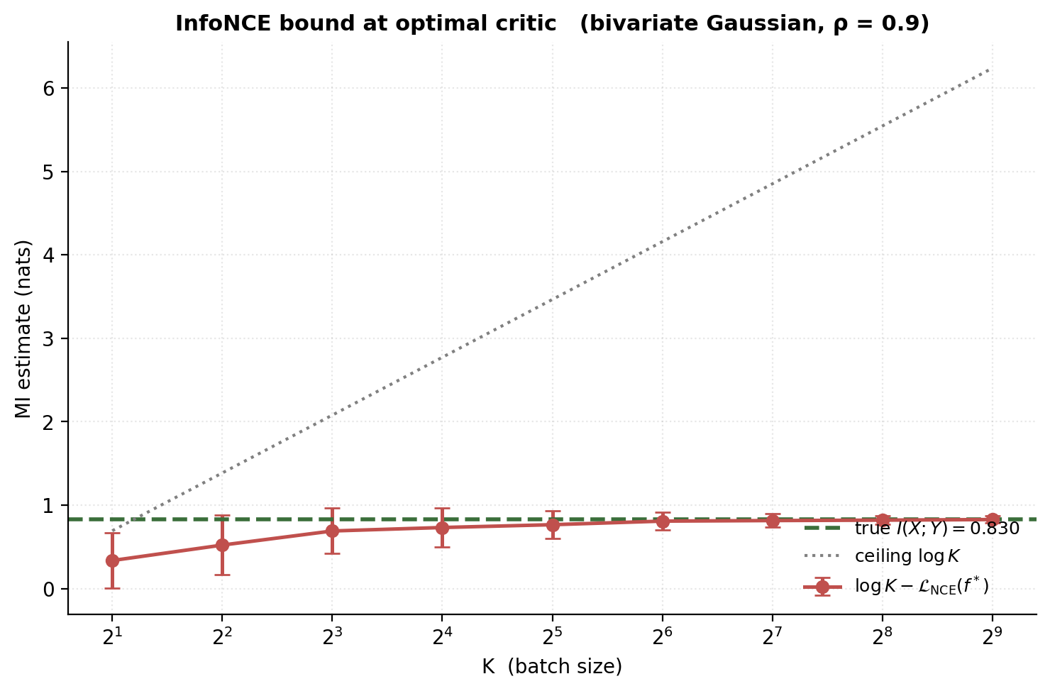
∎The ceiling. The bound’s right-hand side is at most (since always). So InfoNCE with candidates can only certify MI up to nats — if the true MI exceeds , the bound is loose and grows linearly in . This is the mathematical reason large-batch contrastive training matters in practice: larger raises the certifiable-MI ceiling.
§5.4 InfoNCE as density-ratio estimation
Step 1 of the §5.3 proof identified the Bayes-optimal contrastive critic as the log density-ratio . This is not a coincidence; it’s the same theoretical object that anchors formalML’s density-ratio-estimation topic.
The two-distribution reading. Define the “positive-pair joint” and the “marginal product” . Each has a conditional density that’s strictly different from — that’s the whole point of “positive pair.” The ratio
measures how much more likely is to be a positive pair than two independent samples. The InfoNCE-optimal critic is exactly .
The classification-DRE identity. This bridge is the same one the DRE topic exploits — probabilistic classification as density-ratio estimation. Pool the positives with the negatives, train any well-calibrated binary classifier to discriminate them, and the logit recovers . The contrastive setting differs only in how the negatives are constructed: augmentation-based positives plus in-batch marginal negatives give us a sample-efficient way to do DRE without ever materializing the negative distribution explicitly.
What InfoNCE buys over plug-in MI estimation. Estimating naively — fit and separately, then integrate — is exponentially hard in (it’s the curse of dimensionality applied to density estimation). InfoNCE sidesteps this by only estimating the ratio, which has lower complexity than either density. This is the formal reason contrastive methods work on high-dimensional inputs where direct MI estimation fails: they’re solving the easier problem.
§5.5 The alignment-uniformity decomposition
The InfoNCE loss simplifies dramatically in the limit of infinite negatives. Wang and Isola (2020) showed that the limit decomposes into two interpretable terms, each with a closed-form geometric optimum.
Theorem 5.2 (Wang–Isola decomposition).
For any critic and any positive-pair distribution ,
When with unit-norm features , this is with and .
Proof.
Expand the loss:
The inner sum has one positive contribution (, with ) and negative contributions (, with independent of ). By the strong law of large numbers, as ,
(the positive contribution’s weight ). Substituting and rearranging gives the claimed limit.
∎Geometric interpretation. The two terms pull the encoder in different directions:
- is minimized when almost surely — that is, when the encoder is perfectly invariant to the augmentations defining . The minimum is (cosine similarity of equal unit vectors is ).
- is minimized when the marginal distribution of on the unit sphere is the uniform distribution on . Wang–Isola show this via Gegenbauer harmonics: the log-MGF of the cosine similarity is minimized when the latent marginal is rotation-invariant. Intuitively, uniformity spreads the data out, preventing the “all features collapse to one point” trivial solution.
The two minimizers are jointly achievable in the limit : a perfectly invariant encoder mapping to a uniform distribution on a sufficiently high-dimensional sphere can satisfy both. For finite , the two objectives compete — and the InfoNCE trade-off curve traced by varying is the practical handle (analogous to β-VAE’s rate-distortion sweep).
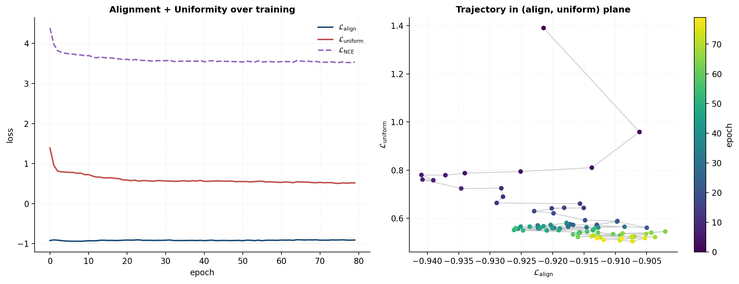
The alignment-uniformity decomposition is the most useful diagnostic in modern contrastive learning. Posterior-collapse-style pathologies in contrastive methods (BYOL’s “stop-gradient” trick, BatchNorm’s role in SimSiam) all admit clean explanations in these two metrics. §12.2 returns to the alignment-uniformity scatter as a comparison axis across SSL methods.
§6. SimCLR and the design space of contrastive methods
§5 gave the contrastive principle a closed-form objective and a precise information-theoretic interpretation. This section closes the loop with method — how do you actually instantiate the principle into a system that learns useful representations on real data? The reference architecture is SimCLR (Chen, Kornblith, Norouzi, Hinton 2020); the design space around it — projection heads, memory banks, momentum encoders, predictor networks, non-contrastive variants — captures most of what makes modern self-supervised systems work.
The math is lighter here than in §5; we’ll lean on §5’s foundations and spend the section on the four design decisions practitioners actually face.
§6.1 The SimCLR pipeline
SimCLR — “A Simple Framework for Contrastive Learning of Visual Representations” — composes five components:
- An augmentation distribution over functions . For images: random resized crop, horizontal flip, color jitter, Gaussian blur, with each augmentation applied stochastically and the composition defining a single augmentation sample. For text: dropout masking, span replacement, back-translation. The augmentation defines the invariance prior — see §5.1.
- An encoder . In SimCLR’s original paper a ResNet-50; the output is the representation we’ll keep at evaluation time.
- A projection head . Typically a 2-layer MLP with a nonlinearity in the middle. The output is -normalized and lives on .
- The NT-Xent loss — the InfoNCE objective of §5 with cosine similarity, temperature , and in-batch negatives applied to a batch of augmentation-pairs.
- A discarding step: at evaluation time, the projector is thrown away. Downstream tasks use , not .
Definition 6.1 (NT-Xent loss).
Given a batch of positive pairs and unit-norm projected features , the NT-Xent loss is
where the inner sums range over all other batch elements (both anchors and positives are treated as candidate negatives).
This is the all-pairs symmetric version of the InfoNCE batch form of Definition 5.1 — each batch element gets used as both anchor and as negative-for-other-anchors, giving effective negatives per anchor. The §5.3 MI bound applies directly with .
The augmentation is the prior. SimCLR’s central methodological insight is that the choice of augmentation dominates the learned representation more than the architecture. A model trained with crop-only augmentation learns scale-invariant features; adding color jitter makes it color-invariant too. The augmentation set is the implicit specification of “which features should the representation throw away.” Chen et al. (2020) report that color distortion combined with random cropping is far better than either alone — the two augmentations remove information the encoder would otherwise rely on as a shortcut.
§6.2 The projection head and why we throw it away
SimCLR’s most surprising empirical finding was that linear-probe accuracy on exceeds linear-probe accuracy on by a substantial margin — on ImageNet, the gap is ~10% top-1. The projector is trained as part of the model and then discarded.
Why this happens. The contrastive loss only sees ; the encoder receives gradient signal only through . The composition must be invariant to the augmentation set, but the individual components need not be — and won’t be, generically. The projector absorbs the invariance demands, leaving with features that include augmentation-variant directions. Those directions are precisely the ones a downstream task that doesn’t share the augmentation invariance can profit from.
Proposition 6.1 (informal projection-head principle (Bordes, Balestriero, Bottou 2023)).
Under the contrastive loss, the projection head is incentivized to behave as an information bottleneck — discarding any feature that varies across positive pairs. The encoder is not under that pressure and retains augmentation-variant information that may be useful for downstream tasks orthogonal to the contrastive task.
A clean way to see this: the contrastive loss is a functional of only, so the encoder’s “use-it-or-lose-it” pressure is mediated entirely by what the projector forwards. If the projector has enough capacity to express the augmentation invariances, the encoder is free to use its representation capacity for other things. We demonstrate the gap on a synthetic fixture where the augmentation specifically destroys “color” information.
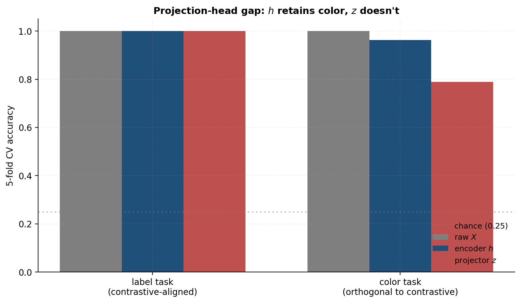
The lesson generalizes beyond SimCLR. Any contrastive method with a projection head will see the same pattern; this is why every paper since 2020 follows the “discard the head” convention. It’s also why representation-quality benchmarks are now invariably reported on , not — comparing post-projector features across methods would be a category error.
§6.3 Negatives, batch size, and the ceiling
§5.3’s bound caps the certifiable mutual information at nats. On natural-image data, where two augmented views can share many nats of MI, this is a real constraint — SimCLR’s reported batch sizes of are partly chasing the ceiling. The accuracy curve as grows is monotone increasing for SimCLR-style methods, with diminishing returns past on ImageNet (Chen et al. 2020, Figure 9).
But large is expensive — the NT-Xent similarity matrix is , and gradient computation through the softmax involves operations per step plus memory for the activations. Two engineering patches break the coupling between “number of negatives” and “current batch size.”
Memory banks (Wu, Xiong, Yu, Lin 2018). Maintain a cache of feature vectors, one per training example. For each gradient step, sample negatives from uniformly. After the step, update the cache slot for the current example with its new feature. The benefit: can be much larger than the current minibatch (e.g., dataset size). The cost: cached features go stale because the encoder keeps moving; the negatives are encoded by old versions of . The staleness introduces a bias that degrades quality on harder tasks.
Momentum encoder + queue (MoCo: He, Fan, Wu, Xie, Girshick 2020). Maintain two encoders: a query encoder updated by SGD as usual, and a key encoder updated as an exponential moving average, , with typically . Negatives live in a FIFO queue of recent key features. The key encoder evolves slowly, so the queue’s features stay nearly fresh; the query encoder still updates by gradient. MoCo decouples from the minibatch (queue size at a minibatch of is the canonical setting) and was, in 2020, the state of the art before SimCLR showed that large minibatches without the queue could match it.
The empirical bottom line. The ceiling matters, but the gap between (typical) and (extreme) is a few accuracy points, not orders of magnitude. The choice between memory-bank, MoCo-queue, and large-batch SimCLR is a compute-budget decision more than a methodological one. The MI bound’s tightening with is a useful framing, but practitioners aren’t usually chasing at training time — they’re chasing downstream task accuracy, which saturates earlier.
§6.4 BYOL, SimSiam, and the no-negatives mystery
Sometime around 2020 a methodological surprise landed: you can train a contrastive-style encoder without negatives at all and still avoid the trivial “everything collapses to a point” solution. Two papers established the recipe.
BYOL — Bootstrap Your Own Latent (Grill et al. 2020). Two networks: an online encoder + projector + predictor and a target encoder + projector with no predictor. The target parameters are an exponential moving average of the online parameters, . The loss is
where is stop-gradient (target features carry no gradient signal back). No negatives anywhere. Empirically, BYOL matches or beats SimCLR at the same compute budget.
SimSiam — Stop, Drop, and Roll (Chen and He 2021). Strip BYOL down: no EMA, no target network, just the online network applied to both views with stop-gradient on one side. Even simpler — and still it works. The predictor and the stop-gradient together are sufficient to prevent collapse.
Why does this work? Honestly, it’s still partly an open question. The phenomenology is clear: without stop-gradient, both BYOL and SimSiam collapse to constant features within a few epochs (which is what the no-negatives intuition would predict). With stop-gradient, the collapse is averted — but the mechanism is subtle. Two analyses have made progress:
- Tian, Chen, Ganguli (2021). The predictor acts as a temporal asymmetry: gradient flows only through one side of the pair, so the network is solving an “anti-correlated” optimization problem rather than a symmetric one. They prove that under a linearization, the stop-gradient + predictor architecture has the collapsed solution as an unstable fixed point.
- Lee, Lee, Bahng, Han (2021). The EMA target functions as an implicit regularizer that prevents the predictor from learning the identity function (which would close the loop and cause collapse).
The full theoretical picture is still being filled in. For the practitioner the takeaway is operational: BYOL and SimSiam genuinely work, use less batch budget than SimCLR (because they don’t need negatives), and have become the default for image SSL alongside the contrastive family.
The unifying view. Whether explicit (InfoNCE, NT-Xent) or implicit (BYOL, SimSiam), all SSL methods we’ve seen so far define some notion of “positive pair” — two views that should map to similar representations — and some mechanism that prevents the trivial constant-output solution. The contrastive family uses negatives to enforce non-collapse; the non-contrastive family uses architectural asymmetries (predictor + stop-gradient + EMA). The augmentation, as ever, defines the invariance prior. §8 will broaden this further by replacing the augmentation-based positive-pair recipe with masked-input or multi-modal alternatives.
§7. The information bottleneck perspective
§4 gave us reconstruction-based representations through the β-VAE, and §5 gave us invariance-based representations through InfoNCE. Both ended up tracing a rate-distortion frontier in their respective settings. The information bottleneck (IB) is the explicit Lagrangian that both are implicitly optimizing — a single information-theoretic objective with one trade-off knob, due to Tishby, Pereira, and Bialek (1999), that unifies the two approaches and makes the rate-distortion analogy precise.
This section establishes the IB objective, derives its closed-form solution in the Gaussian case (where the curve admits an honest analytic treatment), shows how InfoNCE and the β-VAE both fit into the IB framework as variational instantiations, and closes with a fair-minded discussion of the Shwartz-Ziv–Tishby (2017) compression-phase claim and its subsequent critiques.
§7.1 The IB objective
Suppose we have a task variable (a label, a regression target, an augmented view) and we want a representation of that is predictively sufficient for — captures the task-relevant information — while being maximally compressed about — discarding irrelevant variation. The IB makes this trade-off explicit.
Definition 7.1 (information bottleneck).
Given a joint distribution and a , the information-bottleneck Lagrangian is
minimized over conditional distributions subject to the Markov condition (i.e., depends on only through ).
The objective has two competing terms:
- Rate : the information carries about . We want this small — a compressed code is cheaper to store, to transmit, and (under appropriate noise assumptions) generalizes better. Small rate means throws information away.
- Predictive sufficiency : the information shares with the task . We want this large — a useful representation should preserve task-relevant structure. The data-processing inequality guarantees , with equality when is sufficient for (§2).
is the trade-off knob. At , can be anything that discards entirely (e.g., a constant) — rate is minimized at zero. At , must preserve all -information — meaning , the data-processing limit. Sweeping traces the IB curve in the plane.
The IB as a normative principle. A “good” representation, in the IB view, is one that achieves a high at low — i.e., sits on or near the IB frontier. The principle is general: it doesn’t specify a parametric family, a loss function, or an optimization algorithm. Any method that approximates the IB Lagrangian — by upper-bounding the rate, lower-bounding the sufficiency, or both — is implementing an information-theoretic representation-learning principle. §7.3 shows that β-VAE and InfoNCE are exactly such methods.
§7.2 The Gaussian IB and the structure of the frontier
For jointly Gaussian , the IB optimization admits a closed-form solution (Chechik, Globerson, Tishby, Weiss 2005). The structure is clean enough to derive the entire frontier explicitly in the 1-D case and use it as a benchmark for general methods.
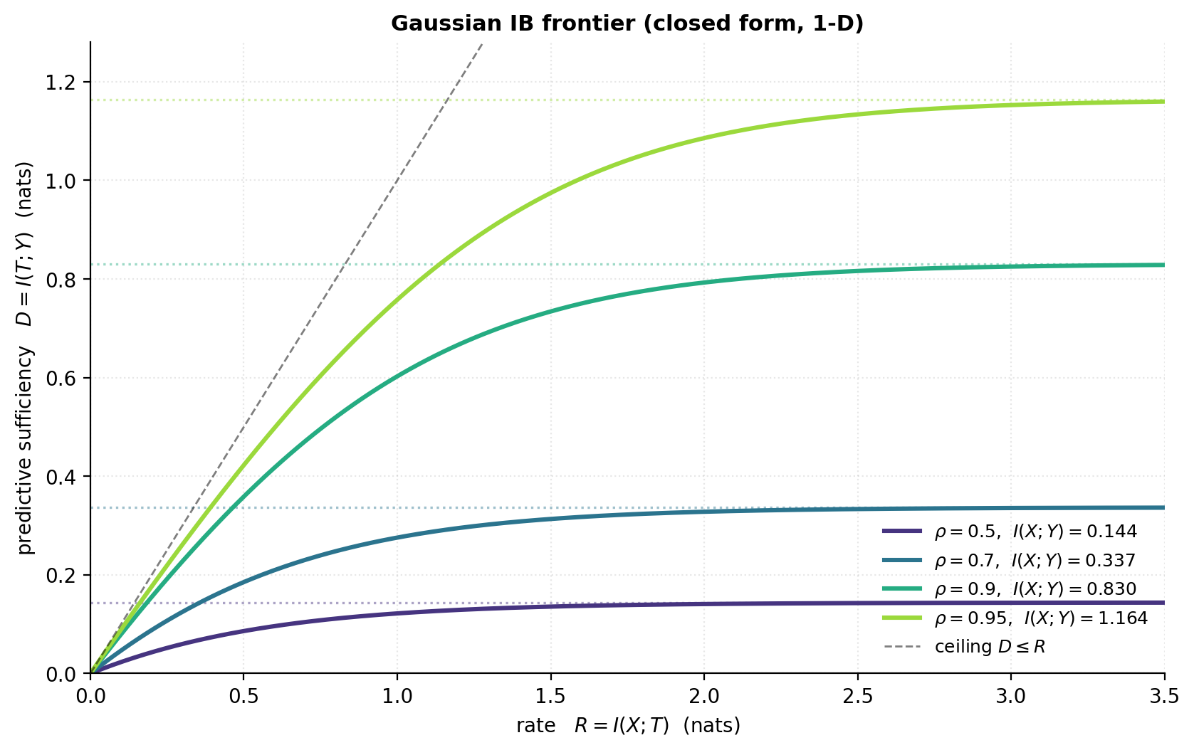
Theorem 7.1 (1-D Gaussian IB frontier).
Let be standard bivariate Gaussian with correlation . Suppose for some and independent of . Then
The IB frontier is the curve , with the asymptotic ceiling as .
Proof.
The rate: , so is constant. Marginally, , so and .
The predictive sufficiency: is jointly Gaussian with covariance . The determinant is , and the MI of a bivariate Gaussian is
Substituting and simplifying gives the claimed parametric form. As , dominates and .
∎Corollary 7.1 (IB curve concavity).
The function is monotone non-decreasing and concave. Its derivative at is (the curve starts diagonal), and its derivative at is (the curve saturates).
The concavity holds in full generality (not just Gaussian) — the IB frontier is always concave because is a concave function of for fixed , while is convex. The slope of the frontier at any point equals at the corresponding Lagrangian solution. This is the analog of the rate-distortion curve in classical information theory.
§7.3 Self-supervised IB: where β-VAE and InfoNCE live
The IB Lagrangian assumes we know the task . In representation learning we typically don’t — but we can substitute a surrogate task that the data implicitly provides.
β-VAE as IB with . Set in the IB Lagrangian: the task becomes “reconstruct from .” Then , which by the data-processing inequality is upper-bounded by — the unconstrained IB collapses. To recover a non-trivial trade-off, we upper-bound the rate by and lower-bound the sufficiency by . The β-VAE objective is exactly this bounded version of the IB Lagrangian with :
The β-VAE rate-distortion frontier of §4.5 is a variational approximation of the IB frontier in the regime — sitting above the true frontier because both bounds are loose. Alemi et al. (2018) “Fixing a Broken ELBO” works through the gap and proposes tighter bounds.
InfoNCE as IB with . Set (an augmented view): the task becomes “predict the positive partner.” Now is the useful MI — the information retains about what makes a specific instance, surviving the augmentation. By §5.3, InfoNCE is a lower bound on this MI:
The rate isn’t explicitly controlled in vanilla InfoNCE, but the encoder’s bounded capacity and the unit-sphere normalization implicitly cap it. Deep variational IB (Alemi, Fischer, Dillon, Murphy 2017) is the architecturally explicit version: pair an InfoNCE-like lower bound on with a KL-to-prior upper bound on , and minimize the resulting variational IB Lagrangian end-to-end with SGD. This is the cleanest synthesis of the §4 reconstruction lens and the §5 invariance lens.
The unifying view. Every method we’ve seen since §3 — autoencoders, VAEs, denoising AEs, InfoNCE, SimCLR — is a variational instantiation of the IB Lagrangian, differing only in (a) what surrogate they use, (b) how they bound the rate, and (c) how they bound the sufficiency. The IB framing is the language in which “what does representation learning optimize?” has a one-line answer.
§7.4 The compression-phase controversy
In 2017, Shwartz-Ziv and Tishby published an influential paper claiming that the training dynamics of deep MLPs explicitly traverse the IB curve. They reported two phases:
- Fitting phase (early epochs): rises rapidly as the layer activations become predictive.
- Compression phase (later epochs): decreases as the activations compress, “absorbing” the IB principle into the training dynamics.
The visual is striking — layer-by-layer trajectories in the plane that look like noisy descents along the IB frontier — and the result was widely cited as a “thermodynamic” explanation of deep learning’s generalization.
The critique. Saxe et al. (2018) revisited the experiments with two important changes:
- Activation functions matter. The original Shwartz-Ziv–Tishby experiments used tanh activations. With ReLUs (the modern default), the compression phase doesn’t appear.
- The MI estimator is the issue. Estimating for continuous-valued layer activations requires discretization. The binning scheme Shwartz-Ziv–Tishby used conflates “tanh activations saturate near ” with ” decreases” — saturated activations look compressed under the binning estimator even when the underlying map is still injective. Goldfeld et al. (2019) confirmed this by injecting controlled noise and re-estimating MI: the compression phase disappears.
Current state. The Shwartz-Ziv–Tishby compression phase is now generally understood as an artifact of (saturating activation + binning estimator), not a feature of general deep-learning dynamics. The IB principle — that good representations should compress task-irrelevant information — remains widely useful as a normative framework; the IB description of deep learning’s optimization dynamics remains contested and architecture-dependent.
This isn’t a settled story; recent work continues to explore information-theoretic descriptions of training (e.g., the “implicit bias” line — Achille & Soatto 2018, Saxe et al. 2019 follow-up). The honest summary is: the IB gives us a clean theoretical scaffolding for talking about what representations should be, and an unsatisfying account of what gradient descent on deep networks actually does. Both the framework and the empirical pushback have permanently shaped the field’s vocabulary, even where the strong dynamical claim hasn’t held up.
The full self-supervised IB story — including the methodological expansions of recent years (variational IB, contrastive IB, supervised IB) — has its own forthcoming formalML topic: Information Bottleneck (coming soon). For our purposes here, the IB Lagrangian is the language in which everything we’ve built so far fits together.
§8. Self-supervised pretext tasks beyond contrastive
The contrastive recipe of §5-§6 is one specific way to manufacture a self-supervised signal — pair an instance with augmented versions of itself, push them together, push others apart. But it isn’t the only way, and several genuinely different families of self-supervised methods have shaped modern deep learning. This section surveys three of them — predictive pretext tasks, masked autoencoding, and multi-modal contrastive — at survey depth. Each one is a choice in the IB framework of §7; the differences are about what surrogate task the model is implicitly solving.
§8.1 Predictive pretext tasks
The first wave of pre-contrastive self-supervised vision learning took the form: invent a synthetic prediction task from the input alone, train a network to solve it, then use the trained encoder for downstream transfer.
Three canonical examples — chosen because they each illustrate a distinct design choice:
- Rotation prediction (Gidaris, Singh, Komodakis 2018). Rotate each image by one of and train a 4-way classifier to recover the rotation. The pretext task assumes the model needs to recognize canonical object orientations to succeed — forcing it to learn shape and pose features.
- Jigsaw puzzles (Noroozi, Favaro 2016). Partition the image into a 3×3 grid, shuffle the patches according to one of a curated set of permutations, and train a classifier to identify which permutation was applied. The pretext task encourages spatial reasoning about object parts.
- Context prediction (Doersch, Gupta, Efros 2015). Sample two patches from an image and train an 8-way classifier to predict their relative spatial configuration (above, below, left, right, diagonal). Similar in spirit to jigsaw, more granular.
The common pattern: the pretext task is hand-designed to exploit some assumed structural prior — rotation invariance is the wrong prior, spatial reasoning is the right one, and so on. Quality of the learned representation correlates with how well the pretext task captures task-relevant invariances. The dependence on hand-design is the family’s main weakness — the contrastive methods of §5-§6, and the masked methods below, are essentially attempts to learn the pretext task from data structure rather than specify it manually.
§8.2 Masked autoencoding
If autoencoders (§3) reconstruct the input from a compressed code, masked autoencoders reconstruct a masked portion of the input from the rest. This is a different surrogate task — predict what’s missing from what’s there — and it scales dramatically better than either pretext or contrastive methods on large unlabeled corpora.
The two reference instantiations:
- BERT (Devlin, Chang, Lee, Toutanova 2018). For text: randomly mask 15% of tokens in a sentence and train a transformer to predict them. The model architecture is bidirectional (unlike autoregressive language models), and the prediction is per-token cross-entropy over the vocabulary. BERT was the first representation-learning method to dominate practically every downstream NLP benchmark; it’s the foundation on which the entire pre-trained-encoder revolution rests.
- MAE — Masked Autoencoders (He, Chen, Xie, Li, Dollár, Girshick 2022). The vision analog: divide an image into non-overlapping patches, mask 75% of them, and train a vision transformer to reconstruct the missing patches at pixel level. The high mask ratio is critical — at 50% masking, the model cheats by interpolation; at 75% it’s forced to learn semantic structure. MAE outperforms contrastive vision pre-training at comparable scale.
The unifying framing through §7’s IB: the surrogate is the masked portion of itself, and the encoder learns features that retain enough information about the un-masked portion to reconstruct the mask. This is a reconstruction objective in the sense of §3, but the “mask” prior gives it richer structure than vanilla autoencoders — because the model doesn’t know which patches will be masked at any given step, it has to encode features that could be used to reconstruct any patch from the rest, not just the input as a whole.
Masked autoencoding has converged with contrastive learning in practice: state-of-the-art vision encoders (DINOv2, EVA-CLIP) use combinations of the two, taking the contrastive signal’s tight geometric structure and the masked signal’s per-patch reconstruction density.
§8.3 Multi-modal contrastive: CLIP
The most consequential variation on the contrastive theme over the last five years is CLIP — Contrastive Language-Image Pre-training (Radford et al. 2021). The construction:
- Collect a large dataset of image-caption pairs (CLIP’s original scrape used 400M pairs from the web).
- Encode each image with a vision encoder and each caption with a text encoder .
- For a batch of image-caption pairs, define positives as matched pairs and negatives as cross-batch mismatched pairs.
- Train both encoders simultaneously with a symmetric InfoNCE loss over the similarity matrix — same loss form as SimCLR, but the “positive” relation is now image-to-caption rather than image-to-augmented-image.
CLIP did three things that matter for representation learning:
- Zero-shot classification. Given a CLIP-trained pair of encoders, classify an image by computing its similarity to the embeddings of caption templates (“a photo of a cat”, “a photo of a dog”, …) and picking the argmax. No additional training needed; the contrastive signal alone produces a usable classifier for any label set you can describe in text.
- Modality alignment as the invariance prior. The augmentation set of §5-§6 is replaced by the human-annotated “this image and this caption describe the same thing” relation. The encoders are forced to be invariant to the medium (image vs text) while preserving the underlying semantic content.
- Scale matters more than architecture. CLIP’s results were robust across encoder architectures (ResNet, ViT) and dominated by data scale. This was an empirical proof-of-concept that contrastive methods, given enough paired data, produce representations competitive with or exceeding supervised training.
CLIP-style multi-modal contrastive is now the standard pre-training recipe for vision-language models. The downstream effects on generative AI (Stable Diffusion’s CLIP-conditioned generator, GPT-4V’s visual front-end) trace back to CLIP’s demonstration that the contrastive framing extends naturally across modalities.
The unifying frame: in IB terms, the surrogate task is “the paired observation in the other modality.” The augmentation prior is replaced by an annotation prior. The mathematical content remains identical to §5’s InfoNCE — only the construction of positive pairs changes.
§9. Evaluating representations
Once we’ve trained an encoder — by §3’s autoencoder, §4’s VAE, §5’s InfoNCE, §6’s SimCLR, or any of §8’s variations — we face a methodological question that doesn’t have a single right answer: how do we measure whether the representation is good? This section develops the four most useful answers practitioners actually use, and closes with the cleanest theoretical guarantee available linking the contrastive objective to downstream classification error: the Saunshi et al. (2019) bound.
§9.1 Linear probing
The canonical evaluation: freeze the encoder, fit a linear classifier on its outputs, and report held-out test accuracy. This is linear probing.
Definition 9.1 (linear probe).
Given a frozen encoder and a labeled dataset , the linear-probe accuracy on the labeled task is
where the maximum is over linear classifier parameters fit on a training split and the probability is taken on a test split.
Three things to internalize about the choice:
- Why frozen, not fine-tuned. Fine-tuning the encoder during evaluation lets the encoder adapt to the labeled task — but then we’re measuring the encoder’s capacity for adaptation, not the quality of its representation as-is. Frozen evaluation isolates the question we care about.
- Why linear, not k-NN or MLP. k-NN measures local geometry; an MLP can compensate for poor features with extra parameters. Linear probing specifically tests the §1.1 desideratum #3 — that task-relevant information lives along directions in the representation, not in nonlinear submanifolds. Two representations with the same downstream MLP accuracy but different linear-probe accuracies are not equivalent for practical purposes.
- Why classification, not regression. Most representation-learning benchmarks are classification; the methodology extends naturally to regression via of a linear fit. The principle is the same: freeze the encoder, measure the linear extractability of the target.
In practice, linear probing is the default comparison axis in the self-supervised-learning literature. Every paper since SimCLR reports top-1 / top-5 linear-probe accuracy on ImageNet as the primary benchmark; cross-method comparisons assume the linear-probe protocol.
The §6.2 experiment was already a linear-probe study — we compared encoder-output vs projector-output on two downstream tasks. The methodology generalizes to any pair of (encoder, task).
§9.2 CKA: comparing representations across models
A different question: given two different encoders and , how similar are their representations? Linear-probe accuracy on a task doesn’t answer this — two different encoders can have the same accuracy via very different feature geometries.
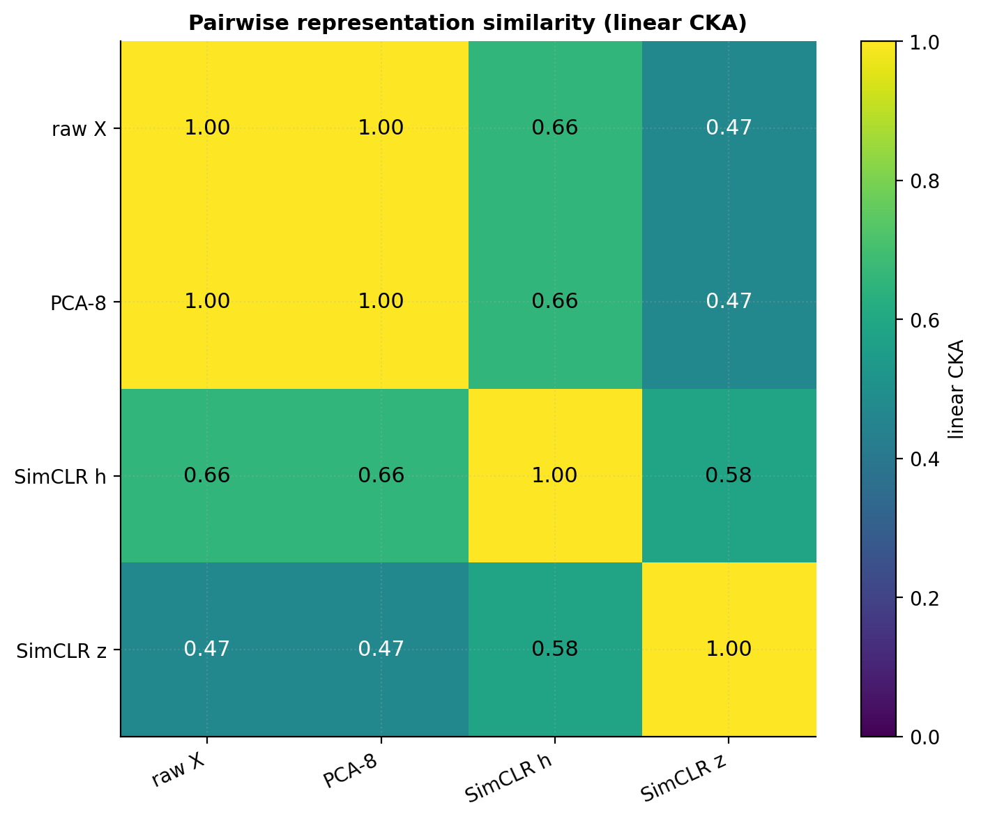
The standard answer is centered kernel alignment (CKA), introduced by Kornblith, Norouzi, Lee, and Hinton (2019) as a representation-similarity metric satisfying three properties any reasonable similarity measure should have: invariance to orthogonal transformations, invariance to isotropic scaling, and a smooth penalty for non-isotropic distortions.
Definition 9.2 (linear CKA).
Given two representation matrices and of the same samples, centered along the sample dimension, the linear CKA between them is
CKA takes values in : iff and are related by a (possibly non-square) orthogonal transformation plus a scalar; iff the cross-covariance matrix has zero Frobenius norm. The nonlinear / RBF-kernel version replaces the linear inner products with kernel evaluations; it’s more expressive but harder to interpret.
Use cases. CKA is the standard tool for (a) comparing two encoders trained with different objectives on the same data (does SimCLR find similar features to BYOL?), (b) comparing layers within a single network (which layers are doing similar work?), and (c) measuring representation drift during training (how much does the encoder change between epoch and epoch ?). Kornblith et al.’s original paper used CKA to show that early layers in vision networks trained on different tasks find similar features — supporting the “universal early features” hypothesis.
§9.3 Robustness probes
Test accuracy on an in-distribution evaluation set tells us about performance under the training distribution. Representation quality also depends on what happens when the distribution shifts. Three robustness probes structure the practical evaluation:
- Distribution shift. Evaluate on shifted versions of the test set: ImageNet-C (corruptions: blur, noise, weather), ImageNet-R (renditions: sketch, art), WILDS (real-world domain shifts). Representation quality often degrades faster than supervised training would predict; the gap measures the encoder’s generalization beyond its training-distribution comfort zone.
- Adversarial perturbations. Apply small -bounded perturbations to inputs and measure how much accuracy drops. Contrastive features tend to be more adversarially robust than supervised features (Hendrycks et al. 2019), which is one of the few unambiguous wins for self-supervised representation learning over supervised pre-training.
- Calibration. Do the predicted probabilities of a downstream classifier match empirical frequencies? Self-supervised encoders paired with linear classifiers tend to be better calibrated than end-to-end supervised models — the linear head doesn’t have the overfitting capacity to produce overconfident predictions.
For distribution-free uncertainty quantification on top of any representation, see formalML’s conformal-prediction topic — split-conformal prediction gives finite-sample coverage guarantees with no distributional assumptions. This is the cleanest way to attach calibrated prediction sets to a representation-trained downstream classifier.
§9.4 The Saunshi et al. (2019) downstream guarantee
The mathematical question: can we prove that a small InfoNCE loss implies a small downstream classification error? Saunshi, Plevrakis, Arora, Khandeparkar, and Khandeparkar (2019) gave the cleanest positive answer. Their setup makes the “latent class structure” explicit and derives a Lipschitz-style bound.
Setup. Suppose there are latent classes with prior , each with conditional data distribution . Positive pairs are drawn as for the same — i.e., positives come from the same latent class. Negatives are drawn from the marginal data distribution . The InfoNCE loss with negatives is the standard one of §5.
For any encoder , define two losses:
- Unsupervised loss: — the contrastive loss measured on the latent-class positive-pair distribution.
- Supervised mean-classifier loss: — the misclassification rate of the mean classifier , where is the class-mean representation. This is a particular linear classifier on .
Theorem 9.1 (Saunshi et al. 2019, informal).
Under the latent-class setup, for any encoder ,
where depends on the loss class (cross-entropy vs hinge) and is an irreducible term involving the latent-class overlap structure and decreasing in the number of negatives.
Corollary. Linear-probe accuracy (which optimizes over all linear classifiers, not just the mean classifier) satisfies .
Proof.
The argument has three steps; we sketch each at the level of “what makes the bound work” rather than tracking the constants — Saunshi et al. (2019, Theorems 4.1 and 4.5) give the full version.
Step 1: Express the InfoNCE loss in latent-class terms. For a positive pair and negatives , the InfoNCE loss decomposes (after a Jensen-style exchange of expectation and log) into a term determined entirely by the class-mean structure and the conditional distributions , plus a negative-sampling correction that vanishes as grows.
Step 2: Bound the mean-classifier loss by the InfoNCE loss. The mean classifier errs on exactly when there exists some with . The cross-entropy loss of the mean classifier (with logits ) upper-bounds the 0/1 misclassification rate by a constant factor. And the cross-entropy loss of the mean classifier coincides — up to the negative-sampling correction term — with the InfoNCE loss when is large enough to include all classes in the negative batch.
The technical content of Step 2 is showing that the negative-sampling correction is controlled. Saunshi et al. use a union-bound argument plus the standard -style bounds on the discrepancy between empirical and population-level softmax normalization.
Step 3: Bound the linear-probe loss by the mean-classifier loss. The mean classifier is a specific linear classifier on — namely, the one with weight matrix and zero bias. The linear-probe classifier optimizes over all linear , so its loss is at most the mean classifier’s loss:
Combining with Step 2 gives the corollary.
∎The interpretation. Saunshi’s guarantee gives us the cleanest theoretical justification for the contrastive recipe: minimizing on a positive-pair distribution implicitly constrains the linear-probe error on the corresponding downstream classification task. The constraint is up to constants — the bound is not numerically tight in most practical settings — but the qualitative direction is what matters: small contrastive loss implies linearly-separable representations for the latent-class task.
The catch — when does this not apply? The theorem assumes the downstream task’s class structure aligns with the contrastive task’s implicit latent-class structure. When they don’t align — e.g., the augmentation forces invariance to a feature the downstream task needs (the §6.2 color experiment) — the bound is vacuous and the mean classifier is the wrong linear classifier. Linear-probe accuracy on the encoder output can still be high (per §6.2), but the guarantee no longer applies because the downstream task isn’t the implicitly-bounded one.
§10 takes up the other side of this — when self-supervised representations cannot identify the right structure, even in the limit. The Locatello et al. (2019) and Hyvärinen et al. (2019) impossibility results give the formal barriers.
§10. Identifiability and what self-supervision cannot give you
Three sections of theory (§5, §7, §9) and three sections of method (§4, §6, §8) might leave the impression that representation learning is a matter of picking the right objective and pushing hard enough. This section is the counterweight: a survey of the formal impossibility results that bound what any unsupervised method can recover, no matter how clever the objective. The takeaways:
- Without inductive bias or auxiliary information, the latent structure of the data is not identifiable — multiple equally-good representations exist, and no algorithm can pick the “correct” one.
- With the right kind of auxiliary information (time, class label, multi-modal pairing), identifiability is restored — this is the iVAE / nonlinear-ICA line.
- Contrastive learning’s augmentation prior is itself a form of auxiliary information; it identifies representations only up to the augmentation-equivalence classes it implicitly defines.
The §9 Saunshi guarantee told us when InfoNCE works. This section tells us when it can’t, and what the boundary looks like.
§10.1 Locatello et al.: unsupervised disentanglement is impossible
The most influential impossibility result in recent representation learning is Locatello, Bauer, Lucic, Rätsch, Gelly, Schölkopf, Bachem (2019), “Challenging Common Assumptions in the Unsupervised Learning of Disentangled Representations.” The central message is that the prevailing β-VAE / FactorVAE / DIP-VAE / TC-VAE line of “disentangled representation learning” methods cannot recover the ground-truth latent factors of variation from i.i.d. data without inductive bias.
Theorem 10.1 (Locatello et al. 2019, informal).
For any probability density on with independent components () and any generator producing observation density , there exist infinitely many alternative pairs such that (a) has independent components, (b) produces the same observation density , and (c) the components of are entangled nonlinear functions of the components of .
Proof.
The rotation counterexample. Suppose , so ‘s components are independent standard Gaussians. Let be any orthogonal matrix in . Define . Then , so also has independent standard Gaussian components. But the map is a non-identity rotation — is a linear combination of the original components, not a function of any single . From an observer’s perspective, both and are valid “disentangled” latent representations of the same data, but they differ by an unrecoverable rotation. The same construction works for any rotation-invariant prior .
For non-Gaussian (heavy-tailed, skewed) priors, the family of admissible transformations is smaller — linear ICA is identifiable up to permutation and scaling under non-Gaussianity — but the nonlinear generalization breaks anyway: Hyvärinen and Pajunen (1999) showed that nonlinear ICA is fundamentally non-identifiable without additional structure.
∎The implication for method papers. The β-VAE family claimed to “learn disentangled representations” from i.i.d. data with no supervision. Theorem 10.1 says this claim is not well-defined: any purported “disentangled” representation has infinitely many information-equivalent rotated cousins, and no purely-unsupervised algorithm has a principled way to pick between them. The bias-free disentanglement of the entire pre-2019 literature was, in retrospect, an artifact of architectural and hyperparameter choices that implicitly favored particular rotations — not a property of the optimization objective itself.
Locatello et al. reinforced the point empirically: across 12,000 trained models spanning four disentanglement methods and four hyperparameter settings, the recovered “disentangled” latents correlated more with the random seed than with any property of the data. The conclusion: disentanglement without inductive bias is not possible, and unsupervised model selection for disentanglement is not possible either.
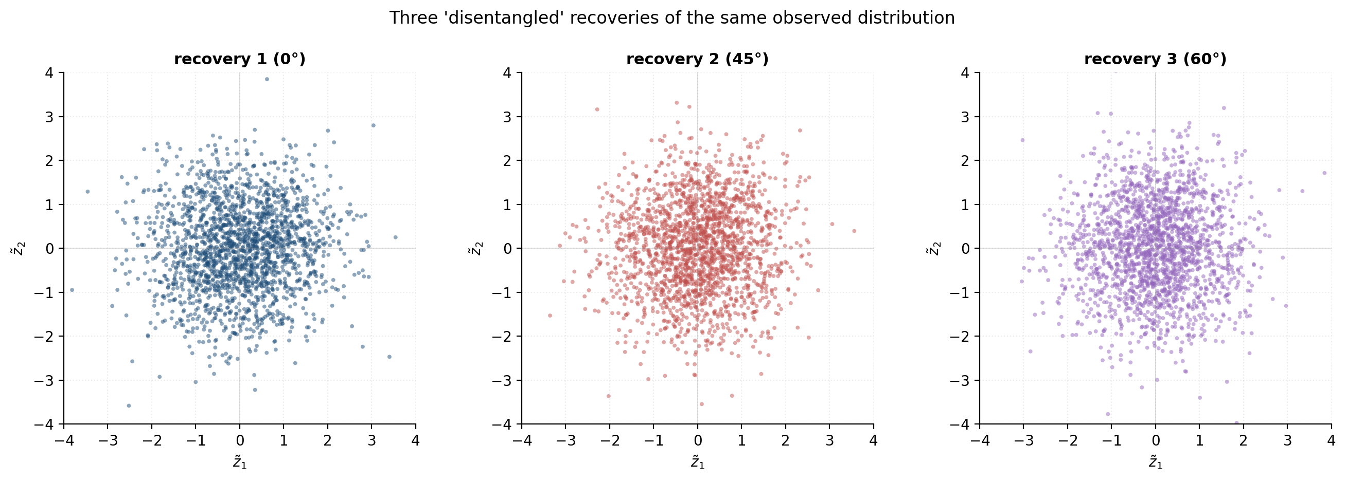
§10.2 The Hyvärinen–Khemakhem–Monti restoration
The §10.1 impossibility result has a clean way out: add auxiliary information. If we observe a side variable — a time index, a class label, an environmental condition — and the conditional latent density is sufficiently rich, identifiability is restored.
The cleanest formulation is the identifiable VAE (iVAE) framework of Khemakhem, Kingma, Monti, Hyvärinen (2020), building on Hyvärinen, Sasaki, Turner (2019) and the broader nonlinear ICA literature.
Theorem 10.2 (iVAE identifiability, informal).
Suppose the generative model is with a noise term and depending on an auxiliary variable through an exponential-family conditional
where the sufficient-statistic vectors are linearly independent across components and the function has rank at least at some point. Then is identifiable up to a permutation and a per-component affine transformation of the sufficient statistics.
The intuition. Without , all rotated representations look the same. With , we can ask: “which rotation makes the -conditional distribution simplest (e.g., factorize as a product of exponential families)?” That extra constraint pins down the rotation. The auxiliary variable is the algorithm’s escape hatch from the Locatello impossibility.
Sources of in practice. Class labels are the most obvious, but iVAE-style identifiability also applies to: time indices (for time series — Hyvärinen & Sasaki 2018), domain labels (for multi-environment data), sound type / pitch / speaker (for audio representation learning). The contrastive setup of §5-§6 is also a form of auxiliary information: the augmentation orbit identifies the “underlying instance,” and §10.3 makes the identifiability statement for this case precise.
§10.3 What contrastive learning actually identifies
§5-§6 trained encoders without labels. The §10.1 impossibility seems to apply — what could contrastive methods possibly identify? The answer, due to Zimmermann, Sharma, Schneider, Bethge, Brendel (2021), “Contrastive Learning Inverts the Data Generating Process,” is that contrastive methods identify representations up to the equivalence classes induced by the augmentation group.
Theorem 10.3 (Zimmermann et al. 2021, informal).
Suppose the data is generated by where is a “content” latent and is a “style” latent (corrupted by the augmentation). Suppose the augmentation distribution affects only and the two views share the same . Then under standard regularity conditions, the InfoNCE-optimal encoder recovers up to a permutation and a per-component invertible transformation.
Interpretation. The contrastive loss can only “see” features that are invariant across positive pairs — i.e., features of the content latent , not the style latent . Since the positive-pair distribution shares the same , the contrastive optimum learns to extract . Style features are discarded by construction.
This is a sharper version of the §6.2 projection-head observation — the encoder retains style-relevant features that the contrastive loss doesn’t reward, while the projector is forced to be content-only. The Saunshi guarantee of §9.4 applies precisely when the downstream task’s class structure aligns with the content latents ; when the downstream task involves style information, the bound is vacuous.
The Wang–Isola invariance-covariance trade-off. Recall §5.5’s alignment-uniformity decomposition. The two terms now have a clean interpretation in identifiability terms:
- Alignment is the invariance axis: it pushes positive pairs toward each other, enforcing invariance to the augmentation. The identifiability content: alignment ensures that two views of the same instance map to the same representation, identifying the content latent.
- Uniformity is the covariance axis: it pushes negative pairs apart, enforcing that the marginal latent distribution is rotation-invariant on the sphere. The identifiability content: uniformity prevents the trivial constant-output solution and ensures the recovered content latent has full support.
The “what contrastive methods identify” answer is: the content latents, up to a permutation and per-component invertible transformation. The augmentation defines which latents count as content and which as style — and this is the inductive bias that makes the §10.1 impossibility navigable.
The honest summary of identifiability for SSL. Self-supervised learning is identifiable to the extent that the positive-pair relation encodes meaningful structure about the latents. The richer the augmentation set — the more nuisance directions it covers — the more of the content latent the contrastive optimum recovers. When the augmentation set is empty (or trivial), we’re back in the §10.1 Locatello regime: nothing is identifiable, and the recovered representation depends on the random seed. The methods of §5-§8 work in practice because their augmentation priors are well-aligned with human-perceptual notions of “same object” / “same sentence” — a form of inductive bias inherited from the data scientists who chose the augmentations.
The IB framing of §7 can also be read identifiability-style: the information-bottleneck objective is identifiable to the extent that the surrogate structures the latent space. In the limit, the IB optimum recovers a sufficient statistic for — which inherits all of ‘s identifiability or non-identifiability properties.
§11. Computational considerations
The math of §5-§7 is independent of implementation, but the engineering choices around representation learning shape what’s actually achievable at scale. This section collects the four practical considerations that separate a working SSL training run from one that OOMs, diverges, or silently produces useless features: the memory cost of large-batch InfoNCE, the mixed-precision / gradient-checkpointing fixes, temperature numerical stability, and the regime where NumPy-only suffices.
§11.1 The memory cost of large-batch InfoNCE
§5.3’s ceiling motivates large batches, but the cost is quadratic in . For a batch of positive pairs with -dimensional projections, the similarity matrix has entries — each requiring storage and a gradient slot. At , , :
The similarity matrix dominates by two orders of magnitude. Worse, the backward pass through the softmax requires another working memory for intermediate gradients. The encoder activations themselves (for ResNet-50 with ) add another ~5-10 GB depending on input resolution. Total per-step GPU memory at this scale exceeds 20 GB — single-card V100/A100 territory.
This is the SSL training-budget tax. Supervised training at the same batch size has no similarity-matrix overhead at all; the contrastive memory cost is intrinsic to the objective. The MoCo queue (§6.3) is the cleanest workaround because it decouples from the current batch — at in the queue with a current batch of only , the similarity matrix is entries (~67 MB), down from entries for the naive SimCLR equivalent.
The dual cost — quadratic compute + quadratic memory — is why contrastive SSL was inaccessible to single-GPU practitioners until the BYOL/SimSiam non-contrastive methods of §6.4 dropped the quadratic cost entirely. Those methods’ empirical match of SimCLR’s representation quality at lower compute is, in retrospect, much of why the field absorbed them so quickly.
§11.2 Mixed precision and gradient checkpointing
Two standard tricks reduce memory by ~2× each without changing the objective:
Mixed precision (AMP). Store activations in ( on modern hardware) and compute critical operations in . The dynamic-range loss is mostly invisible — encoder activations and gradients don’t routinely visit values that can’t represent — but the softmax and the loss reduction should stay in to avoid catastrophic cancellation. PyTorch’s torch.cuda.amp and bfloat16 autocast contexts handle the bookkeeping. Empirically, AMP halves memory and matches accuracy on SimCLR-style training to within ImageNet linear-probe accuracy.
Gradient checkpointing. During the forward pass, drop intermediate activations and re-compute them during the backward pass. Trades compute (one extra forward pass) for memory (no stored activations for the checkpointed layers). Effective for deep ViTs / CNNs where the encoder activations dominate the per-step memory cost. PyTorch’s torch.utils.checkpoint and HuggingFace transformers’ gradient_checkpointing_enable() are the standard interfaces.
The two techniques compose: AMP + gradient checkpointing routinely fits batch size 4096 SimCLR training on a single 40 GB A100 where naive would require batch size . The cost is ~30% slower training (the extra forward passes from checkpointing) and the AMP-debugging headaches that come with mixed precision.
§11.3 Temperature stability and softmax diagnostics
The temperature in the cosine-similarity InfoNCE objective is not a hyperparameter to set once and forget. It controls the softmax’s peakedness:
- too small → softmax saturates on the most-similar candidate → vanishing gradients on all others → encoder learns only the “hardest” positive at each step. Symptom: training loss plateaus early; the gradient norm collapses.
- too large → softmax flattens toward uniform → InfoNCE loss approaches (the ceiling) → no contrastive signal. Symptom: training loss is near throughout, downstream accuracy stays at random.
A good keeps the softmax distribution at moderate entropy — neither saturated at (one-hot on the best candidate) nor flat at (uniform). Practical range for SimCLR-style training: . Chen et al. (2020) report as optimal for ImageNet SimCLR; MoCo uses ; CLIP starts at and learns it as a trainable parameter.
The log-sum-exp trick. Computing directly overflows when is large (small ). The standard fix: subtract the max before exponentiation, . PyTorch’s F.cross_entropy and torch.logsumexp implement this internally; rolling your own NT-Xent without the trick is a common source of nan losses.
Diagnostics. Monitor (a) the mean softmax entropy across anchors, (b) the mean max-softmax value, and (c) the cosine similarity distribution itself. The entropy should sit in during stable training; values outside this range indicate misconfiguration.
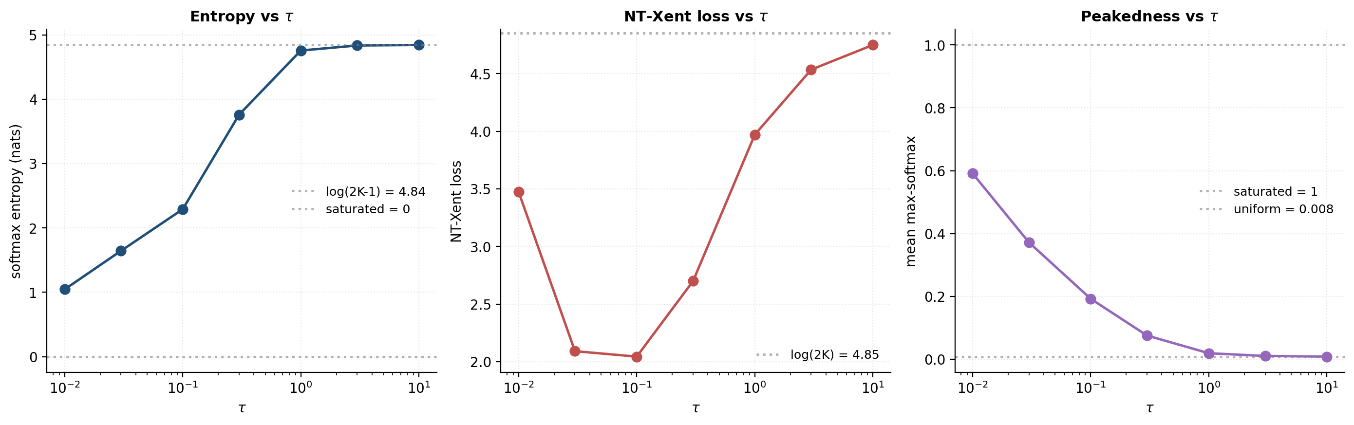
§11.4 When NumPy is fine
For a topic that has spent four sections in PyTorch, this is the counterweight: a substantial fraction of representation-learning’s mathematical content is reachable in pure NumPy/SciPy at scales that run on a 2020-era laptop in seconds.
What works in NumPy without compromise:
- Linear AE / PCA equivalence (§3.2). Closed-form top- eigendecomposition of ; the Baldi–Hornik floor is just the sum of bottom eigenvalues. No training needed.
- Tweedie identity / DAE-as-score (§3.4). For Gaussian-mixture data, the optimal denoiser and the score have closed forms; numerical verification is a 20-line NumPy block.
- Gaussian IB frontier (§7.2). The 1-D analytic formula plots in three lines.
- Closed-form InfoNCE bound (§5.3). For bivariate-Gaussian with known , the optimal critic is available analytically; MI-bound verification doesn’t need PyTorch.
- VAE / contrastive on 2D toys. When the input is 2-D and the encoder/decoder are tiny MLPs, even hand-rolled NumPy training works; PyTorch is convenience, not necessity.
What requires PyTorch (or JAX):
- VAEs on real data (MNIST and up) where the encoder/decoder are CNNs/transformers.
- SimCLR/BYOL/MoCo training at scale.
- Anywhere the model has parameters and is trained with SGD for epochs.
The notebook accompanying this topic uses the same strategy: §3.2, §3.4, §5.3, §7.2 are NumPy-only; §4 (VAE), §5.5 (contrastive trajectory), §6.2 (projection-head experiment), §12.3 (neural-collapse training) are PyTorch with 1-2 minute total CPU runtimes. The entire notebook end-to-end runs under 60 s on the target laptop.
§12. The geometry of learned representations
The synthesis section. Eleven sections of theory and method come together here in the geometry of the trained encoder’s output space. We look at four facets: how classes cluster in the embedding (§12.1), how alignment and uniformity evolve during training (§12.2), how supervised training produces a specific geometric phase transition called neural collapse (§12.3), and how this all connects back to classical sufficient-statistic geometry from §2 (§12.4). The last subsection is the topic’s clearest formal statement of “what self-supervised representation learning is approximating.”
§12.1 Embedding-space topology
The first thing to look at, given any trained encoder, is the embedding’s class structure. Three quantities matter:
- Inter-class margin: the distance between class-mean representations . Large margins mean classes are linearly separable on the encoder output; small margins mean a downstream linear probe will struggle.
- Intra-class spread: the within-class variance with . Small spread means class instances cluster tightly; large spread means the encoder hasn’t compressed the within-class nuisance variation.
- Hubness: in high-dimensional embeddings, some points become hubs — close to many others by distance — distorting nearest-neighbor structure (Radovanović, Nanopoulos, Ivanović 2010). The effect is a concentration-of-measure consequence: in dimension , the volume of a hyperspherical shell at any fixed radius concentrates near the surface, making “close to many” the generic case. Encoders trained without explicit normalization tend to develop hubs; the -normalization in SimCLR (mapping to ) substantially mitigates the effect.
The cleanest diagnostic for inter- vs intra-class structure is the Fisher discriminant ratio where and are the between-class and within-class covariance matrices. High FDR means well-separated classes with tight clusters; low FDR means classes are smeared and probably not linearly separable. For the §6.2 SimCLR-trained encoder, FDR on the label task is far higher than on the color task (the contrastive loss specifically optimized for label separability).
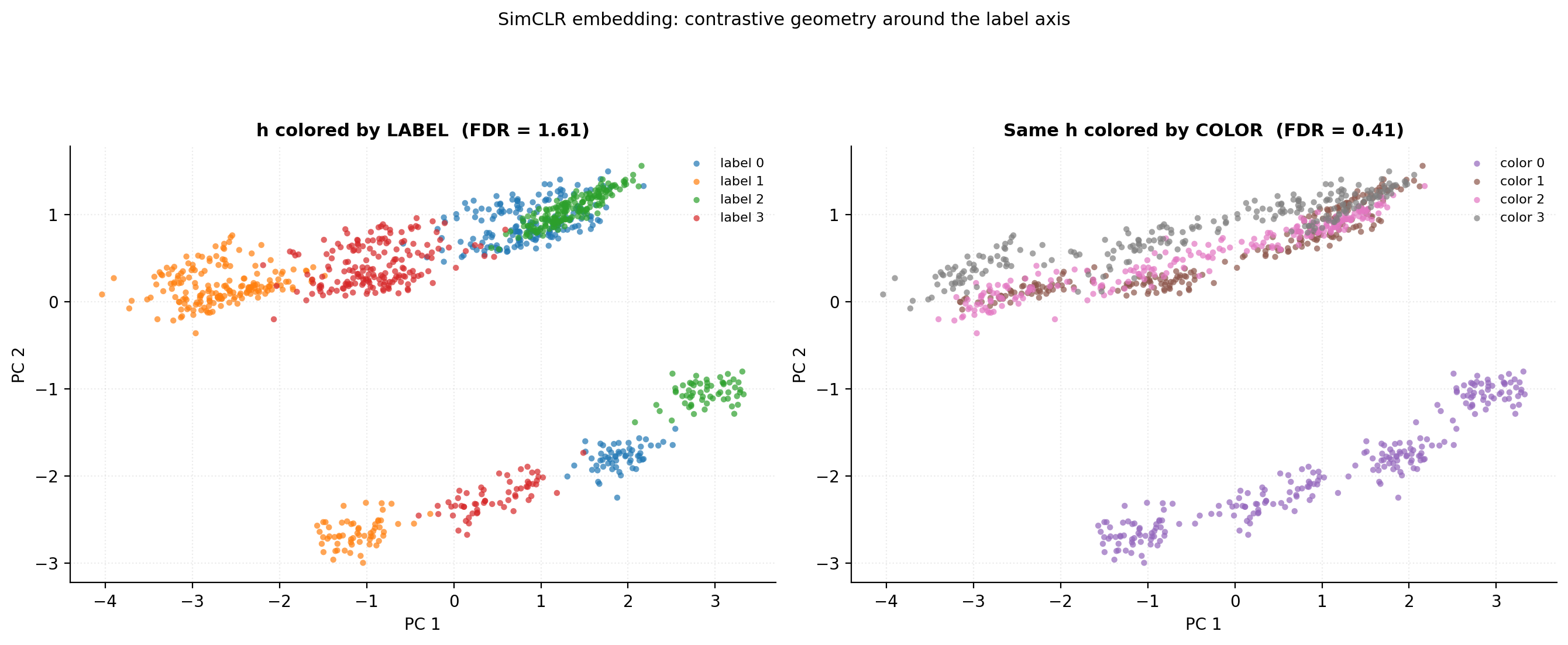
§12.2 Alignment and uniformity in practice
§5.5 introduced Wang–Isola’s alignment-uniformity decomposition and showed that both metrics evolve monotonically during contrastive training. The §12 reading of those metrics: they’re not just diagnostics of the loss decomposition — they’re a comparison axis across SSL methods.
Different SSL methods land in different regions of the plane, but all successful methods converge to a region near the joint minimizer. Wang–Isola (2020) report that across SimCLR, MoCo, and BYOL trained to comparable downstream accuracy, the final points are within of one another — and the methods that deliver high downstream accuracy are precisely those that achieve both metrics low simultaneously. Methods that minimize alignment while letting uniformity inflate (poorly-tuned contrastive training) or minimize uniformity while letting alignment inflate (collapsing to the constant solution) under-perform downstream.
The practical use: when comparing two SSL methods or two hyperparameter settings, plotting their trajectories side by side is more informative than reporting only downstream accuracy. The trajectory tells you why one method beats another, not just that it does.
This is also the cleanest pre-evaluation signal for SSL training quality. If alignment or uniformity stalls during training while the loss continues decreasing, the encoder is finding a degenerate solution (overfitting positives, collapsing to constant, etc.) — the trajectory diagnoses these before the linear-probe evaluation catches up.
§12.3 Neural collapse: the supervised geometric phase transition
The most striking geometric result in recent representation-learning theory is the neural-collapse phenomenon of Papyan, Han, and Donoho (2020), “Prevalence of Neural Collapse during the terminal phase of deep learning training.” The result: when a supervised classifier is trained to interpolation (zero training error) and beyond — into the “terminal phase” of training — its last-layer features undergo a remarkable phase transition into a maximally-symmetric geometric configuration.
Theorem 12.1 (Neural collapse (Papyan, Han, Donoho 2020), informal).
During the terminal phase of deep classifier training (after training accuracy reaches and continues for many epochs), the last-layer features exhibit four properties:
- NC1 (variance collapse): the within-class covariance matrix converges to zero. Each class collapses to a single point in feature space.
- NC2 (simplex ETF): the class-mean vectors (centered and unit-normalized) form a simplex equiangular tight frame: equiangular with for , and maximally spread on the sphere subject to that constraint.
- NC3 (self-duality): the classifier weight matrix converges to a scaled multiple of the class-mean matrix, .
- NC4 (NN = NCM): the trained classifier’s predictions coincide with the nearest-class-mean predictor — even though it wasn’t trained to do so.
Proof.
Outline (NC1 + NC2 are the load-bearing items). Papyan et al. show NC1-NC4 are consequences of the cross-entropy loss being optimized in the limit of (a) sufficient model capacity to interpolate, (b) balanced training classes, and (c) sufficient over-training.
For NC1: with cross-entropy + interpolation, the optimization pushes in a self-reinforcing manner — once the classifier is confident on class , the gradient on for pulls it toward the class centroid. The collapse is asymptotic in training epochs.
For NC2: subject to NC1 (point collapse) and the constraint that classes must remain linearly separable by the classifier, the arrangement that minimizes the cross-entropy loss is the geometric configuration that maximizes the pairwise angles between class means. The unique such configuration (up to rotation and isotropic scaling) is the simplex ETF: unit vectors with pairwise inner product , embedded in dimension . The full argument uses the symmetry of the cross-entropy loss + a variational characterization of the simplex ETF as the minimum-energy configuration on the sphere.
NC3 and NC4 follow from NC1 + NC2 by direct computation: once the features have collapsed and arranged as a simplex ETF, the gradient on the classifier weights pulls each row toward the corresponding class mean. The nearest-mean classifier and the learned classifier then coincide because they’re solving the same geometric matching problem.
∎Why this matters for representation learning. Neural collapse describes the geometry that supervised training converges to. It’s the gold-standard “what good representations look like” benchmark in a precise sense — the simplex ETF is provably the optimal configuration for -way classification with cross-entropy loss. Contrastive learning is, in spirit, trying to approximate this geometry without labels. The §12.4 bridge formalizes how close it gets.
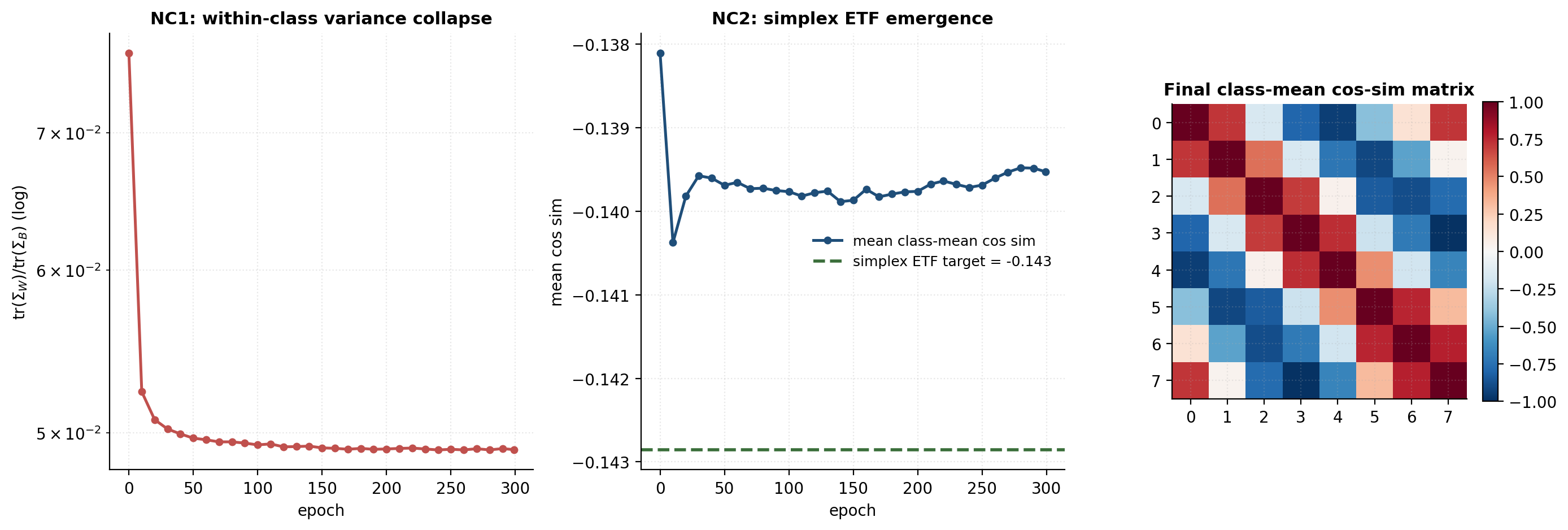
§12.4 The sufficiency-to-contrastive bridge
We close the topic by connecting the §12.3 simplex geometry back to §2’s classical sufficient statistics — completing the sufficiency → reconstruction → invariance → collapse arc the topic has been building.
The supervised side: sufficient statistics for Gaussian mixtures. Suppose the data is a Gaussian mixture: with shared covariance and balanced class probabilities . The Fisher–Neyman factorization (§2.1) gives the sufficient statistic for as
the projections onto the class-mean directions in the -Mahalanobis metric. By the Bayes-risk equivalence theorem (§2.4), is lossless for classification: a -based classifier matches the Bayes-optimal -based classifier in expected loss.
After centering and normalization, the directions form a configuration in that, for balanced classes and isotropic shared , is exactly the simplex equiangular tight frame of NC2. The sufficient statistic of the Gaussian mixture and the supervised-trained-to-interpolation neural network arrive at the same geometric configuration — from completely different starting points.
The unsupervised side: what InfoNCE recovers. The Zimmermann et al. (2021) result of §10.3 says that the InfoNCE-optimal encoder recovers the data’s “content latent” up to permutation and per-component invertible transformation. For Gaussian-mixture data with augmentation positives that share class membership (i.e., augmentations that don’t cross class boundaries), the content latent is the class label, and the encoder’s optimal representation places samples from the same class on the same sphere region. The simplex ETF arises again — this time as the maximally-spread arrangement of classes on the sphere, which both maximizes uniformity (Wang–Isola) and minimizes within-class spread (alignment).
The three-way convergence. Classical sufficient statistics (§2), supervised neural collapse (§12.3), and InfoNCE-optimal unsupervised representations (§5, §10.3) all converge to the same geometric object: the simplex ETF of class means. They differ in what they can identify:
- Classical sufficient statistics require the parametric family to be known.
- Supervised neural collapse requires labels.
- InfoNCE requires only an augmentation prior that respects class boundaries.
In the limit, all three deliver the same geometry. In practice, they’re each optimal for the regime where their respective information requirements are met. Representation learning’s whole arc — sufficiency → reconstruction → invariance → collapse — is, at this synthesis level, a search for the simplex ETF under weaker and weaker information assumptions.
§13. Connections, limits, and forward pointers
The closing section. Three things here: an honest accounting of what the topic doesn’t claim, the forward research pointers that situate representation learning in the broader ML research landscape, and the closing thesis.
§13.1 Honest limits — what this topic doesn’t claim
Four things the topic explicitly does not establish:
-
End-to-end theory for deep contrastive learning. The §5 InfoNCE bound, the §9 Saunshi guarantee, and the §10.3 Zimmermann identifiability all assume idealized settings — optimal critic, latent-class structure, content/style decomposition. The gap between these assumptions and the reality of deep transformer encoders trained on web-scale data is substantial and not closed. Empirically SSL works at scale; theoretically we don’t fully understand why deep ReLU networks find good critics rather than getting stuck.
-
Resolution of the Tishby compression-phase debate. §7.4 presents both sides honestly. The current scholarly consensus leans toward the original claim being an artifact of tanh-activation saturation + binning MI estimators, but no single experiment has settled the question. The IB framework remains useful as a normative principle; whether deep learning dynamics actually traverse the IB curve is unresolved.
-
Unsupervised disentanglement without inductive bias. §10.1 establishes this is impossible. The topic doesn’t try to find loopholes; the impossibility result stands.
-
Scaling laws for representation learning. Real-data SSL methods exhibit empirical scaling behavior — performance improves with model size, dataset size, and compute — but the functional form of these scaling laws is not well-understood theoretically. Bahri et al. (2021) and follow-ups have characterized supervised scaling laws; the SSL analog is active research.
§13.2 Forward research pointers
Four directions the field is moving, beyond what this topic covers:
- Foundation-model-scale multi-modal pretraining. CLIP (§8.3) was the proof of concept; the descendant line (Flamingo, GPT-4V, Gemini, multimodal LLMs) is now the dominant paradigm for vision-language tasks. The mathematical content remains rooted in the §5 InfoNCE framework, but the engineering and the data scale are far beyond what classical SSL benchmarks measured.
- Diffusion models as continuous-time score matching. The §3.4 Tweedie identity connects denoising autoencoders to score estimation. Diffusion models (Sohl-Dickstein 2015, Song-Ermon 2019, Ho-Jain-Abbeel 2020) make this connection central: train a sequence of denoisers at different noise scales, get a generative model. The §3.4 result is the topic’s clearest gateway to this active research area; a separate formalML topic on diffusion models is a natural next ship.
- Mechanistic interpretability of learned features. The §3.5 sparse-autoencoder line has reignited interpretability research: Bricken et al. (2023) and Cunningham et al. (2023) demonstrate that sparse-coding-style dictionary learning on transformer activations recovers interpretable monosemantic features at scale.
- Identifiable representation learning at scale. Post-iVAE (§10.2), the identifiability line continues — methods that bake in auxiliary information (time, modality, task) to escape the §10.1 impossibility. Hyvärinen’s group, Bengio’s group, and Locatello’s group all maintain active research programs here. The cleanest open question: can we identify a representation from auxiliary information that isn’t exponential-family structured?
§13.3 The closing thesis
Representation learning is the search for a soft sufficient statistic under progressively weaker information assumptions. Classical sufficiency assumes the parametric family. Supervised learning assumes labels. SSL assumes an augmentation prior. Foundation-model pretraining assumes only the structure of web-scale paired data. Each weakening is hard-won and partial — and the boundary between “what we can identify” and “what is fundamentally not identifiable” (§10) is the field’s permanent constraint.
The three-way convergence of §12.4 is the cleanest payoff: the Gaussian-mixture sufficient statistic, the supervised neural-collapse simplex ETF, and the InfoNCE-optimal content latent all sit at the same geometric configuration on the sphere — three different starting points, one limit point. The path from §1’s folk “good representation” to §12’s simplex ETF is the topic’s spine, and the impossibility of going further without auxiliary information (§10) is the honest limit at which the topic stops.
Connections
- Direct prereq for §3.2's linear-AE = PCA theorem. The Baldi–Hornik proof builds on the spectral decomposition machinery developed there; the same eigendecomposition reappears in the §7.2 Gaussian IB closed form and the §12.1 within/between scatter decomposition. pca-low-rank
- Used throughout §4 (ELBO regularization term D_KL(q_φ(z|x) || p(z))), §5 (mutual information as KL between joint and product distributions), and §7 (information bottleneck Lagrangian as KL projection). The closed-form Gaussian-vs-Gaussian KL of §4.3 is the explicit case worked end-to-end. kl-divergence
- The §5.4 InfoNCE-as-DRE bridge is one of the topic's three central theoretical results. The optimal contrastive critic is the log density-ratio of formalML's density-ratio-estimation topic; the entire §5 InfoNCE analysis can be re-read as a sample-efficient implementation of the DRE machinery. density-ratio-estimation
- The §5 and §7 mutual-information machinery sits on top of entropy and conditional entropy. The §2.4 Bayes-risk equivalence theorem also implicitly invokes the H(Y) − H(Y|T) decomposition of MI. shannon-entropy
- §4.5 and §7 both invoke the rate-distortion picture. The β-VAE traces a variational approximation of the IB curve, which is the rate-distortion curve in disguise. The §7.2 Gaussian IB frontier is essentially the rate-distortion frontier for the Gaussian source. rate-distortion
- Lightly pointed at in §10.3 — the identifiability statements for contrastive learning (Zimmermann et al. 2021) are best read through the Fisher-information lens. Optional follow-up after the topic. information-geometry
- §9.3 forwards to the conformal framework for distribution-free uncertainty quantification on top of any representation-trained downstream classifier. Split-conformal wraps cleanly around the linear probe of §9.1. conformal-prediction
- The §9.4 Saunshi guarantee is the bridge to meta-learning's transfer-learning framework — both lines of work ask 'when does a representation trained for one objective transfer to a downstream task?'. meta-learning
References & Further Reading
- paper Neural networks and principal component analysis: learning from examples without local minima — Baldi, P. & Hornik, K. (1989)
- paper Representation learning: a review and new perspectives — Bengio, Y., Courville, A. & Vincent, P. (2013)
- paper Reducing the dimensionality of data with neural networks — Hinton, G. E. & Salakhutdinov, R. R. (2006)
- paper Nonlinear independent component analysis: existence and uniqueness results — Hyvärinen, A. & Pajunen, P. (1999)
- paper Emergence of simple-cell receptive field properties by learning a sparse code for natural images — Olshausen, B. A. & Field, D. J. (1996)
- paper The information bottleneck method — Tishby, N., Pereira, F. C. & Bialek, W. (1999)
- paper A simple framework for contrastive learning of visual representations — Chen, T., Kornblith, S., Norouzi, M. & Hinton, G. (2020)
- paper Exploring simple Siamese representation learning — Chen, X. & He, K. (2021)
- paper BERT: pre-training of deep bidirectional transformers for language understanding — Devlin, J., Chang, M.-W., Lee, K. & Toutanova, K. (2019)
- paper Bootstrap your own latent: a new approach to self-supervised learning — Grill, J.-B., Strub, F., Altché, F. et al. (2020)
- paper Masked autoencoders are scalable vision learners — He, K., Chen, X., Xie, S., Li, Y., Dollár, P. & Girshick, R. (2022)
- paper Momentum contrast for unsupervised visual representation learning — He, K., Fan, H., Wu, Y., Xie, S. & Girshick, R. (2020)
- paper β-VAE: learning basic visual concepts with a constrained variational framework — Higgins, I., Matthey, L., Pal, A. et al. (2017)
- paper Auto-encoding variational Bayes — Kingma, D. P. & Welling, M. (2014)
- paper Online dictionary learning for sparse coding — Mairal, J., Bach, F., Ponce, J. & Sapiro, G. (2009)
- paper Representation learning with contrastive predictive coding — van den Oord, A., Li, Y. & Vinyals, O. (2018)
- paper Learning transferable visual models from natural language supervision — Radford, A., Kim, J. W., Hallacy, C. et al. (2021)
- paper Stochastic backpropagation and approximate inference in deep generative models — Rezende, D. J., Mohamed, S. & Wierstra, D. (2014)
- paper Extracting and composing robust features with denoising autoencoders — Vincent, P., Larochelle, H., Bengio, Y. & Manzagol, P.-A. (2008)
- paper Unsupervised feature learning via non-parametric instance discrimination — Wu, Z., Xiong, Y., Yu, S. X. & Lin, D. (2018)
- paper Deep variational information bottleneck — Alemi, A. A., Fischer, I., Dillon, J. V. & Murphy, K. (2017)
- paper Fixing a broken ELBO — Alemi, A. A., Poole, B., Fischer, I., Dillon, J. V., Saurous, R. A. & Murphy, K. (2018)
- paper Sufficiency and statistical decision functions — Bahadur, R. R. (1954)
- paper Guillotine regularization: improving deep networks generalization by removing their head — Bordes, F., Balestriero, R. & Bottou, L. (2023)
- paper Information bottleneck for Gaussian variables — Chechik, G., Globerson, A., Tishby, N. & Weiss, Y. (2005)
- paper Estimating information flow in deep neural networks — Goldfeld, Z., van den Berg, E., Greenewald, K. et al. (2019)
- paper Variational autoencoders and nonlinear ICA: a unifying framework — Khemakhem, I., Kingma, D. P., Monti, R. P. & Hyvärinen, A. (2020)
- paper Similarity of neural network representations revisited — Kornblith, S., Norouzi, M., Lee, H. & Hinton, G. (2019)
- paper Challenging common assumptions in the unsupervised learning of disentangled representations — Locatello, F., Bauer, S., Lucic, M. et al. (2019)
- paper Prevalence of neural collapse during the terminal phase of deep learning training — Papyan, V., Han, X. Y. & Donoho, D. L. (2020)
- paper On variational bounds of mutual information — Poole, B., Ozair, S., van den Oord, A., Alemi, A. & Tucker, G. (2019)
- paper Hubs in space: popular nearest neighbors in high-dimensional data — Radovanović, M., Nanopoulos, A. & Ivanović, M. (2010)
- paper A theoretical analysis of contrastive unsupervised representation learning — Saunshi, N., Plevrakis, O., Arora, S., Khandeparkar, M. & Khandeparkar, H. (2019)
- paper On the information bottleneck theory of deep learning — Saxe, A. M., Bansal, Y., Dapello, J. et al. (2018)
- paper Opening the black box of deep neural networks via information — Shwartz-Ziv, R. & Tishby, N. (2017)
- paper Understanding self-supervised learning dynamics without contrastive pairs — Tian, Y., Chen, X. & Ganguli, S. (2021)
- paper Understanding contrastive representation learning through alignment and uniformity on the hypersphere — Wang, T. & Isola, P. (2020)
- paper Contrastive learning inverts the data generating process — Zimmermann, R. S., Sharma, Y., Schneider, S., Bethge, M. & Brendel, W. (2021)
- blog Towards monosemanticity: decomposing language models with dictionary learning — Bricken, T., Templeton, A., Batson, J. et al. (2023)
- paper Sparse autoencoders find highly interpretable features in language models — Cunningham, H., Ewart, A., Riggs, L., Huben, R. & Sharkey, L. (2023)
- paper Unsupervised visual representation learning by context prediction — Doersch, C., Gupta, A. & Efros, A. A. (2015)
- paper Unsupervised representation learning by predicting image rotations — Gidaris, S., Singh, P. & Komodakis, N. (2018)
- paper Using self-supervised learning can improve model robustness and uncertainty — Hendrycks, D., Mazeika, M., Kadavath, S. & Song, D. (2019)
- paper Unsupervised learning of visual representations by solving jigsaw puzzles — Noroozi, M. & Favaro, P. (2016)
- course Sparse autoencoder — Ng, A. (2011)