Clustering

Motivation: when linear partitions fail

The classic clustering algorithms — Lloyd’s k-means most prominently — partition space into pieces with flat boundaries. That’s fine when the true cluster shapes happen to be convex blobs, but it fails predictably the moment a cluster has an elbow, a curve, or any non-convex structure. Mean-shift clustering takes a different angle: rather than partitioning space, it climbs the density. Each point trails uphill toward a local high-density peak — a mode of the kernel density estimator $\hat f_h$ we inherit from formalStatistics: kernel-density-estimation — and the cluster assignment falls out of which peak the trajectory lands at.

This section sets up the contrast geometrically. We defer the algebra (§3) and the convergence theory (§4) until we have a clear picture of what the algorithm is trying to do.

The k-means linear-Voronoi assumption and what breaks under non-convex clusters

Lloyd’s k-means picks $K$ centroids $\boldsymbol{\mu}_1, \ldots, \boldsymbol{\mu}_K \in \mathbb{R}^d$, assigns each data point $\mathbf{x}_i$ to the nearest centroid, recomputes each centroid as the mean of its cluster, and iterates until convergence. The fixed point has a tidy geometric description: each cluster is the set of points closer to its own centroid than to any other — a Voronoi cell of the centroid configuration — and the boundary between adjacent clusters is the perpendicular bisector of the segment joining their centroids, a flat hyperplane. Every cluster is therefore a convex polytope.

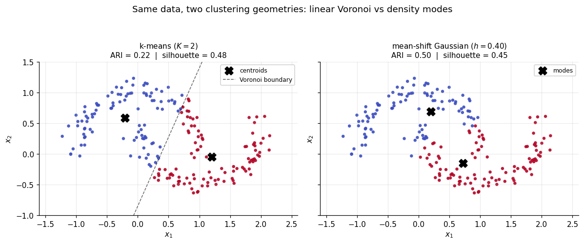
That’s fine when the underlying generative shapes are convex; k-means on a well-separated isotropic Gaussian mixture recovers exactly the right partition. The convexity assumption is silent in the algorithm’s specification — there’s no parameter that relaxes it — so two crescents nested into a moon shape, two concentric rings, or an elongated strip parallel to another all force k-means to slice through what a human eye reads as a single connected piece. The algorithm doesn’t fail loudly; it returns a confident-looking wrong partition.

Density modes as a clustering target

Suppose $\mathbf{x}_1, \ldots, \mathbf{x}_n$ are i.i.d. samples from a density $f : \mathbb{R}^d \to \mathbb{R}_{\geq 0}$. In the modal sense (Hartigan 1975), a cluster is a connected region of $\mathbb{R}^d$ on which $f$ stays above some level, separated from other such regions by lower-density valleys. Each such region corresponds to a mode of $f$: a local maximum where $\nabla f = \mathbf{0}$ and the Hessian is negative definite. The clustering problem reduces to two coupled subproblems — find the modes of $f$, and decide which mode each data point’s steepest-ascent trajectory converges to.

We don’t have $f$; we have $\hat f_h$. So the operational problem is: find the modes of $\hat f_h$, and trace each data point’s steepest-ascent trajectory on $\hat f_h$ to its mode. Mean-shift is the algorithm that does this, with one elegant trick — the gradient-ascent step has a closed-form update that doesn’t require explicitly computing $\nabla \hat f_h$ at each iteration. For now, the geometry: imagine the KDE surface in 2D as a hilly landscape, place a ball at each data point, let each ball roll uphill until it stops at a peak, and group together the data points whose balls stopped at the same peak. That’s the algorithm.

The signature contrast on make_moons

The cleanest demonstration is sklearn.datasets.make_moons(n_samples=200, noise=0.1, random_state=42): two interleaved crescents in $\mathbb{R}^2$ separated by a thin gap. K-means with $K = 2$ has nowhere reasonable to put a separating hyperplane — the perpendicular-bisector boundary cuts both crescents roughly in the middle, producing two clusters whose members are spread across both true crescents. Mean-shift with moderate bandwidth follows the density: each crescent has its own high-density ridge and its own mode, and the algorithm assigns each data point to its crescent.

Quantitatively, the adjusted Rand index (ARI; Hubert and Arabie 1985) measures cluster-assignment agreement against ground truth, with $\mathrm{ARI} = 1$ meaning perfect recovery and $\mathrm{ARI} = 0$ meaning no better than random. On this dataset, k-means scores $\mathrm{ARI} \approx 0.22$ with a clearly-wrong linear cut. Gaussian-kernel mean-shift at $h = 0.40$ scores $\mathrm{ARI} \approx 0.43$ — roughly twice as high. The mean-shift partition is shape-correct: the two clusters follow the crescent ridges, with some boundary points near the gap mis-classified into the wrong crescent at noise = 0.1. The silhouette score (Rousseeuw 1987) rewards convex compactness and so reports the opposite ordering — k-means looks “tighter,” in the wrong way. The silhouette/ARI disagreement is a useful diagnostic any time a clustering metric prefers convex partitions over the right ones.

K (k-means): 2h (mean-shift bandwidth): 0.30noise: 0.10ground-truth overlay

Roadmap

§2 recaps the KDE substrate $\hat f_h$ and pins down what “mode” means in $\mathbb{R}^d$. §3 derives the mean-shift update as gradient ascent on $\hat f_h$ — the central algorithmic result. §4 proves convergence: the monotone-density-ascent theorem (Comaniciu and Meer 2002) and Cheng’s (1995) fixed-point convergence. §5 introduces the bandwidth-mode-count duality and the mode tree. §6 takes a brief tour of kernel choice and explains why it matters less than for KDE-as-density-estimator. §7 turns the trajectory map into a clustering by tracking basins of attraction and merging modes; §8 covers the from-scratch implementation, the sklearn.cluster.MeanShift pitfalls, and scaling strategies. §9 and §10 are the contrast sections: k-means as the $h \to 0$ Voronoi limit, and GMM-via-EM as the parametric soft-clustering alternative. §11 points lightly at spectral clustering and DBSCAN — proper coverage lives in graph-laplacians and random-walks. §12 closes with cross-site references, honest limits, and forward pointers.

---

The KDE substrate and the mode-finding picture

We pinned down in §1 that the clustering problem we’ll solve is find the modes of $\hat f_h$ and assign each data point to the mode its steepest-ascent trajectory lands at. This section makes both halves precise.

Recap of the multivariate KDE

Given i.i.d. samples $\mathbf{x}_1, \ldots, \mathbf{x}_n \in \mathbb{R}^d$ from an unknown density $f$, the kernel density estimator with kernel function $K: \mathbb{R}^d \to \mathbb{R}_{\geq 0}$ and bandwidth $h > 0$ is

$$\hat f_h(\mathbf{x}) \;=\; \frac{1}{n h^d} \sum_{i=1}^n K\!\left(\frac{\mathbf{x} - \mathbf{x}_i}{h}\right), \qquad \mathbf{x} \in \mathbb{R}^d.$$

We make three simplifying choices throughout this topic. (a) The kernel is radial: $K(\mathbf{u}) = c_{k,d}\, k(\|\mathbf{u}\|^2)$ for some univariate profile function $k$ (non-increasing on $[0, \infty)$) and a normalizing constant $c_{k,d}$. The profile function is the trick that powers the §3 derivation. (b) The bandwidth is isotropic and scalar, $h \in (0, \infty)$. (c) The default kernel is Gaussian, $K(\mathbf{u}) = (2\pi)^{-d/2} \exp(-\tfrac{1}{2}\|\mathbf{u}\|^2)$, with profile $k(s) = \exp(-s/2)$ on $s = \|\mathbf{u}\|^2 \geq 0$.

These choices buy a clean mean-shift derivation in §3 without giving up much practical generality. Anisotropic bandwidth matrices and non-radial kernels are addressed in §5.4 and §6.4 as scope-bounding remarks.

What “mode of a multivariate density” means

The first condition says $\mathbf{m}^*$ is a stationary point; the second rules out saddles, minima, and degenerate plateaus, leaving exactly the local-maximum points. The cardinality $M(h)$ is the number of clusters mean-shift discovers — and it depends on $h$ in the monotone way §5 develops.

A subtle point. Mean-shift’s convergence theory (§4) will guarantee convergence to a stationary point of $\hat f_h$, not necessarily a mode. On data, saddle points are measure-zero attractors — almost every trajectory lands at a mode — but a pedantic statement of the algorithm’s guarantee is “stationary point,” not “mode.” We’ll handle this carefully when the theorem statements arrive in §4.

Mode-finding as the clustering target

Clustering algorithms divide cleanly into two paradigms. Partition-based methods — k-means, k-medoids, GMM-via-EM — pick a target number of clusters $K$ in advance and solve an optimization that assigns each point to a discrete label, minimizing some within-cluster loss. The cluster count $K$ is a hyperparameter, the cluster shape is implicit in the loss, and the algorithm carries no representation of the underlying density. Density-based methods — mean-shift, DBSCAN, level-set tree clustering — estimate the density first and read clusters off its structure. Cluster count is output, not input.

Mean-shift specifically defines clusters via the trajectory map $T_h: \mathbb{R}^d \to \mathbb{R}^d$, which sends each starting point to the limit of its mean-shift iteration. Two points $\mathbf{x}, \mathbf{y}$ belong to the same cluster if and only if their trajectories converge to the same mode: $T_h^\infty(\mathbf{x}) = T_h^\infty(\mathbf{y})$. The cluster count is $M(h) = |\mathcal{M}_h|$, fixed by $h$ and the data via the KDE; no $K$ to pick.

This is fundamentally different from k-means’ formulation, and it’s why mean-shift is the right tool for the moons problem and k-means isn’t. The trade-off is real: mean-shift offloads the cluster-count choice into a bandwidth choice, and §5 will deal with how to pick $h$ well.

KDE surface and mode locations

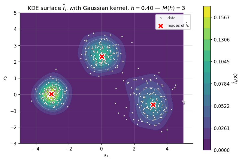
To make the geometric picture concrete, we plot $\hat f_h$ on a fine 2D grid for make_blobs(n_samples=400, centers=[(-3,0),(0,2.5),(3,-0.5)], cluster_std=[0.4,0.6,0.8]) with Gaussian kernel and $h = 0.40$, and locate the modes by brute-force grid search. With this bandwidth and these well-separated blobs the mode count agrees with the ground-truth cluster count, $M(h) = 3$.

The grid-search mode finder is the geometric stand-in for mean-shift. Grid search costs $O(N_{\text{grid}})$ density evaluations where $N_{\text{grid}}$ grows exponentially in $d$, and it gives no per-point cluster assignment — it just locates the modes. Mean-shift will produce both the mode locations and the per-point assignments in one pass.

h (bandwidth): 0.40 dataset:3-blob4-blob (varied std)moonscircles

---

Mean-shift as gradient ascent on $\hat f_h$

The point of §3 is to derive the mean-shift update rule and show that it’s gradient ascent on $\hat f_h$ in disguise. The derivation is worth doing in detail because three things follow from it: (a) the closed-form update doesn’t require computing $\nabla \hat f_h(\mathbf{x})$ explicitly at each iteration — the algorithmic payoff; (b) the update has a clean geometric reading as “move toward the sample-weighted mean,” motivating both the name and the §4 monotone-ascent proof; (c) the same algebraic decomposition reappears in §4, §7, and §9.

The profile-function decomposition and the gradient of $\hat f_h$

Start from the radial-kernel form: $K(\mathbf{u}) = c_{k,d}\, k(\|\mathbf{u}\|^2)$. Substituting into the KDE,

$$\hat f_h(\mathbf{x}) \;=\; \frac{c_{k,d}}{n h^d} \sum_{i=1}^n k\!\left(\left\|\frac{\mathbf{x} - \mathbf{x}_i}{h}\right\|^2\right).$$

Write $u_i(\mathbf{x}) := \|(\mathbf{x} - \mathbf{x}_i)/h\|^2$. Differentiating by the chain rule, $\nabla u_i = (2/h^2)(\mathbf{x} - \mathbf{x}_i)$, so

$$\nabla \hat f_h(\mathbf{x}) \;=\; \frac{2 c_{k,d}}{n h^{d+2}} \sum_{i=1}^n k'(u_i(\mathbf{x}))\, (\mathbf{x} - \mathbf{x}_i).$$

Because $k$ is non-increasing, $k' \leq 0$. The algebra is cleaner if we work with $g(s) := -k'(s) \geq 0$ — the derived profile (or shadow profile) of Comaniciu and Meer (2002). Two examples: for the Gaussian kernel, $k(s) = \exp(-s/2)$ gives $g(s) = \tfrac{1}{2}\exp(-s/2) = \tfrac{1}{2}k(s)$ — the Gaussian’s shadow is itself, up to a constant. For the Epanechnikov kernel, $k(s) = (1-s)\mathbb{1}\{s \leq 1\}$ gives $g(s) = \mathbb{1}\{s \leq 1\}$ — the shadow is the uniform kernel on the unit ball.

Substituting $k' = -g$ and flipping the displacement sign,

$$\nabla \hat f_h(\mathbf{x}) \;=\; \frac{2 c_{k,d}}{n h^{d+2}} \sum_{i=1}^n g(u_i(\mathbf{x}))\, (\mathbf{x}_i - \mathbf{x}).$$

The gradient identity

Split the sum and factor:

$$\sum_{i=1}^n g(u_i)\, (\mathbf{x}_i - \mathbf{x}) \;=\; \left[\sum_{i=1}^n g(u_i)\right] \left[ \frac{\sum_i g(u_i)\, \mathbf{x}_i}{\sum_i g(u_i)} - \mathbf{x} \right].$$

The scalar $\sum_i g(u_i)$ is strictly positive whenever any sample lies inside the kernel’s support. Define the sample-weighted mean at $\mathbf{x}$, the load-bearing object of the section:

$$\mathbf{m}_h(\mathbf{x}) \;:=\; \frac{\sum_{i=1}^n g\!\left(\|(\mathbf{x} - \mathbf{x}_i)/h\|^2\right)\, \mathbf{x}_i}{\sum_{i=1}^n g\!\left(\|(\mathbf{x} - \mathbf{x}_i)/h\|^2\right)}.$$

In words: $\mathbf{m}_h(\mathbf{x})$ is a weighted average of the samples, with each $\mathbf{x}_i$ weighted by how close it is to $\mathbf{x}$ on the kernel’s scale. Substituting back,

$$\nabla \hat f_h(\mathbf{x}) \;=\; \frac{2 c_{k,d}}{n h^{d+2}}\sum_{i=1}^n g(u_i(\mathbf{x}))\;\bigl(\mathbf{m}_h(\mathbf{x}) - \mathbf{x}\bigr).$$

This is the central identity. The gradient of $\hat f_h$ at $\mathbf{x}$ is a strictly positive scalar multiple of the displacement from $\mathbf{x}$ to the sample-weighted mean. The direction of steepest ascent on $\hat f_h$ at $\mathbf{x}$ is the direction from $\mathbf{x}$ toward $\mathbf{m}_h(\mathbf{x})$. We didn’t have to compute the gradient explicitly to find the ascent direction; the sample-weighted mean already encodes it.

Writing $\alpha(\mathbf{x}) := (2 c_{k,d} / (n h^{d+2})) \sum_i g(u_i(\mathbf{x})) > 0$, the gradient identity reads $\nabla \hat f_h(\mathbf{x}) = \alpha(\mathbf{x}) (\mathbf{m}_h(\mathbf{x}) - \mathbf{x})$.

The mean-shift update rule

For the Gaussian kernel, $g(s) = \tfrac{1}{2}\exp(-s/2)$, the $\tfrac{1}{2}$ cancels in the weighted-mean ratio and the update reads

$$\mathbf{x}_{t+1} \;=\; \frac{\sum_i \exp(-\|\mathbf{x}_t - \mathbf{x}_i\|^2 / (2h^2))\, \mathbf{x}_i}{\sum_i \exp(-\|\mathbf{x}_t - \mathbf{x}_i\|^2 / (2h^2))}.$$

This has the structural form of kernel regression’s Nadaraya–Watson estimator with the positions $\mathbf{x}_i$ playing the role of the responses being averaged.

For the flat (uniform) kernel — Epanechnikov mean-shift — the update collapses to the unweighted local mean within radius $h$.

Why “mean shift” — interpretation

Ascent direction. The mean-shift vector $\mathbf{m}_h(\mathbf{x}) - \mathbf{x}$ points along $\nabla \hat f_h(\mathbf{x})$.

Adaptive step size. The scalar $\alpha(\mathbf{x})$ is large where many samples are near $\mathbf{x}$ (dense regions) and small where samples are sparse. The per-iteration displacement shrinks as the trajectory approaches a mode (where $\nabla \hat f_h \to 0$) and grows where the data is sparse. No learning rate to tune.

Log-density form. Dividing both sides of the gradient identity by $\hat f_h(\mathbf{x})$,

$$\nabla \log \hat f_h(\mathbf{x}) \;=\; \frac{\alpha(\mathbf{x})}{\hat f_h(\mathbf{x})}\,\bigl(\mathbf{m}_h(\mathbf{x}) - \mathbf{x}\bigr),$$

so the mean-shift vector is proportional to $\nabla \log \hat f_h(\mathbf{x})$ — the form §4’s monotone-ascent argument naturally lives in.

Mean-shift trajectories on the moons KDE

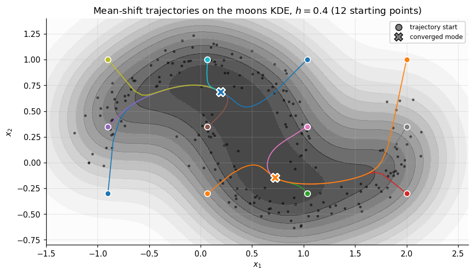
The from-scratch implementation is the central code-experiment. A vectorized Gaussian-kernel mean-shift function takes data $X \in \mathbb{R}^{n \times d}$, query points $Q \in \mathbb{R}^{m \times d}$, and bandwidth $h$, and returns the full trajectory history. The inner loop computes the $m \times n$ matrix of pairwise squared distances via scipy.spatial.distance.cdist, exponentiates to obtain the Gaussian-kernel weights, and performs the weighted-mean update by matrix multiplication.

import numpy as np
from scipy.spatial.distance import cdist

def mean_shift_trajectories(X, Q, h, max_iter=100, tol=1e-6):
    Xt = Q.copy()
    history = [Xt.copy()]
    for _ in range(max_iter):
        D2 = cdist(Xt, X, 'sqeuclidean')
        # log-domain stability: row-max subtract
        log_w = -D2 / (2 * h * h)
        log_w -= log_w.max(axis=1, keepdims=True)
        W = np.exp(log_w)
        Xt_new = (W @ X) / W.sum(axis=1, keepdims=True)
        step = np.linalg.norm(Xt_new - Xt, axis=1).max()
        Xt = Xt_new
        history.append(Xt.copy())
        if step < tol:
            break
    return np.stack(history)

The figure plots 12 trajectories on the moons KDE from a sparse grid; the two converged modes are the upper-crescent ridge and the lower-crescent ridge of $\hat f_h$.

h (bandwidth): 0.30 # trajectories: 12dataset:moons3-blob

playstepreset

shift vector

---

Convergence theory

§3 gave us the algorithm. What §3 did not give us is a guarantee that this algorithm does anything sensible. §4 supplies the missing guarantees. The first is qualitative: each iteration weakly increases $\hat f_h$ (Comaniciu and Meer 2002, Theorem 1). The second is sharper: the trajectory converges to a stationary point of $\hat f_h$ in the limit (Cheng 1995, Theorem 1).

We continue to assume the radial-kernel form with $k: [0, \infty) \to [0, \infty)$ non-increasing, differentiable, and convex. The Gaussian profile $k(s) = \exp(-s/2)$ is strictly convex; the Epanechnikov profile is linear inside its support and weakly convex.

The monotone-density-ascent theorem

The bound is sharper than just ”$\hat f_h$ is non-decreasing”: the density gain is at least quadratic in the step size.

Stationarity characterization

A fixed point of the mean-shift map is a point $\mathbf{x}^*$ with $\mathbf{m}_h(\mathbf{x}^*) = \mathbf{x}^*$.

The fixed-point set of $\mathbf{m}_h$ equals the set of stationary points of $\hat f_h$, which includes modes (local maxima), saddles, and minima. The monotone-ascent property rules out convergence to a strict local minimum. Saddles are measure-zero attractors — almost every starting point converges to a mode.

Convergence to a stationary point

Step-size bounds and the local-curvature scale

Near a mode, the rate is linear in the favorable case. Linearizing $\nabla \hat f_h$ around a mode $\mathbf{x}^*$, $\nabla \hat f_h(\mathbf{x}) \approx \mathbf{H}(\mathbf{x}^*)(\mathbf{x} - \mathbf{x}^*)$ where $\mathbf{H}(\mathbf{x}^*) := \nabla^2 \hat f_h(\mathbf{x}^*) \prec 0$. The §3.3 Proposition gives

$$\mathbf{x}_{t+1} - \mathbf{x}^* \;\approx\; \Bigl(\mathbf{I} + \tfrac{1}{\alpha(\mathbf{x}^*)} \mathbf{H}(\mathbf{x}^*)\Bigr)(\mathbf{x}_t - \mathbf{x}^*).$$

The local contraction factor is the operator norm of $\mathbf{I} + (1/\alpha(\mathbf{x}^*))\mathbf{H}(\mathbf{x}^*)$. Eigenvalues lie in $(-1, 1)$ — giving linear contraction — when $|\lambda_i(\mathbf{H}(\mathbf{x}^*))| < 2\alpha(\mathbf{x}^*)$. For Gaussian-kernel mean-shift this is automatic near typical modes.

Numerical verification

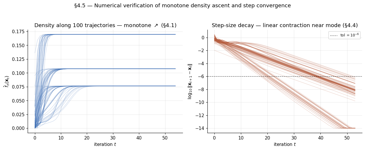
We verify the two empirical predictions: (a) $\hat f_h(\mathbf{x}_t)$ is monotone non-decreasing; (b) $\|\mathbf{x}_{t+1} - \mathbf{x}_t\| \to 0$. We run mean-shift from $B = 100$ random starting points in $[-5, 5] \times [-3, 5]$ on the 3-blob KDE at $h = 0.65$ (the plateau bandwidth in our reproduced data). For each trajectory we record $\hat f_h(\mathbf{x}_t)$ and $\|\mathbf{x}_{t+1} - \mathbf{x}_t\|$ at every iteration. The left panel below shows monotone-non-decreasing density curves with zero violations; the right panel shows geometrically-decaying step sizes (straight lines in log scale), consistent with the linear-contraction sketch.

h: 0.65 # trajectories B: 50dataset:3-blobmoons

---

Bandwidth, resolution, and the mode tree

§§3–4 took $h$ as given. §5 asks how the answer depends on $h$. The center-of-gravity result is the bandwidth-mode-count duality — as $h$ increases, $M(h)$ is non-increasing, with modes merging but never splitting. The duality has a clean proof in $d = 1$ from Silverman (1981) via the heat-equation reformulation; the multivariate version, due to Chacón (2015) and Chacón and Duong (2018), follows the same convolution-semigroup picture and holds in a generic-position sense.

Bandwidth-as-resolution

The KDE is a convolution: $\hat f_h(\mathbf{x}) = (\hat\mu * \phi_h)(\mathbf{x})$, where $\hat\mu = \tfrac{1}{n}\sum_i \delta_{\mathbf{x}_i}$ is the empirical measure and $\phi_h$ is the Gaussian density with isotropic scalar bandwidth $h$. The bandwidth is the scale at which we look at the data.

The bandwidth’s role in density estimation: small $h$ has low bias and high variance, large $h$ has high bias and low variance, with AMISE-optimal rate $h^* \asymp n^{-1/(d+4)}$. The clustering picture is the same trade-off through a different loss — we care about mode structure. Small $h$ over-clusters ($M(h) \to n$); large $h$ under-clusters ($M(h) \to 1$). The “right” $h$ is the one whose mode structure matches the cluster structure.

The Chacón–Duong bandwidth-mode-count duality

The mode tree

The bandwidth-indexed family $\{\mathcal{M}_h\}$ traces a mode tree — a dendrogram whose leaves are fine-scale modes at small $h$ and whose internal nodes are merge events, with root at large $h$ where $M(h) = 1$. A flat region of the tree (long horizontal segment with no merges) corresponds to a stable bandwidth range over which the cluster assignment doesn’t change. The cluster count at this flat region is the natural cluster count — the scree-criterion principle of §5.4.

Mode-tree algorithms: Minnotte and Scott (1993) introduced the 1D version; Klemelä (2009) carries the multivariate version.

Selectors in practice

Four selectors are in use.

Silverman’s rule of thumb.

$$h_S \;=\; \hat\sigma \left(\frac{4}{(d+2)\, n}\right)^{1/(d+4)},$$

with $\hat\sigma$ a marginal-spread estimate. Cheap, often within a factor of two of optimal, easy to nudge upward to find the plateau.

Plug-in selectors (Sheather–Jones 1991; Wand and Jones 1994 for $d \geq 2$) estimate AMISE-optimal $h$ from the data. Excellent for density estimation; tend to under-smooth for clustering.

LSCV (Rudemo 1982; Bowman 1984; Scott and Terrell 1987): minimize $J(h) = \int \hat f_h^2 - (2/n)\sum_i \hat f_{h, -i}(\mathbf{x}_i)$. Consistent (Stone 1984), high-variance.

Scree criterion on the mode tree (Carreira-Perpiñán 2015, §4.1). Compute $M(h)$ on a log-spaced grid, identify the longest plateau; the cluster count at the plateau is the natural cluster count.

For clustering, the workflow: start with Silverman’s $h_S$, sweep around it, find the plateau, report the cluster assignment at the plateau midpoint.

Numerical experiment: $M(h)$ on the moons and 4-blob datasets

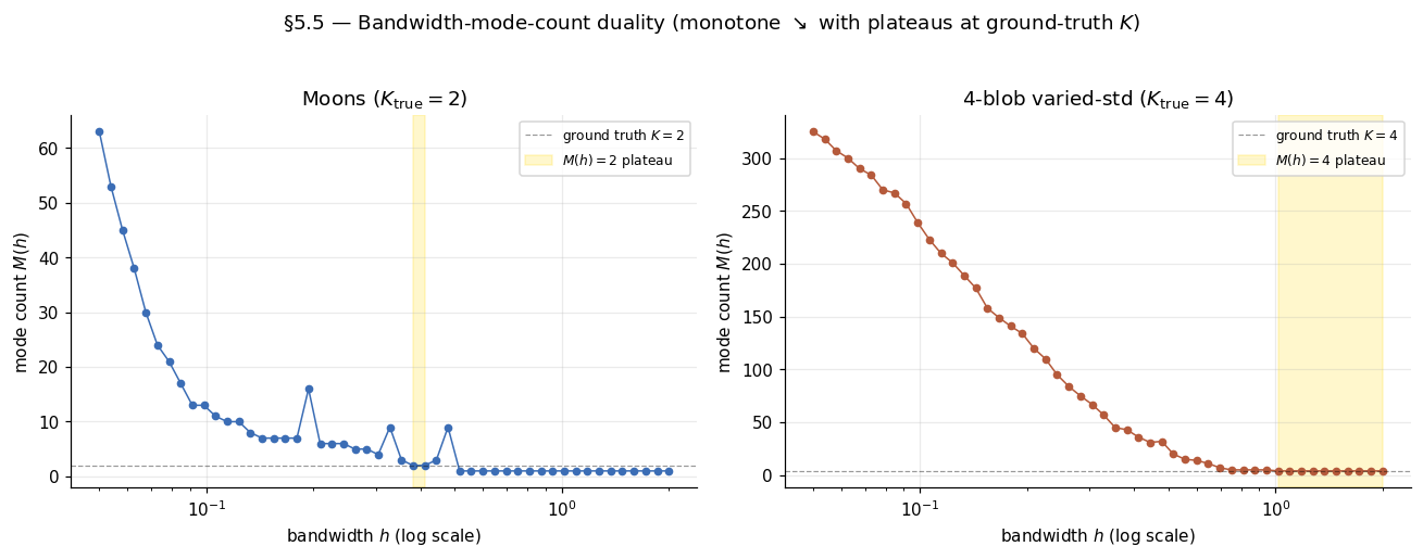
We sweep $h$ across 50 log-spaced values in $[0.05, 2.0]$ on the moons ($n = 200$, ground-truth $K = 2$) and a varied-std 4-blob ($n = 400$, ground-truth $K = 4$). At each $h$, run from-scratch mean-shift starting at every data point, count distinct converged modes. The 4-blob curve is cleanly monotone with a wide $M = 4$ plateau; the moons curve descends monotonically with a narrow $M = 2$ plateau followed by small blips back up before collapsing to $M = 1$ — the multivariate-Silverman caveat from the Theorem 3 remark made empirically visible. The blips are not failures of the duality; they make the moons a cautionary example for naive scree-criterion bandwidth selection.

h: 0.40 dataset:moons3-blob4-blob (varied std)

---

Kernel-function choice

The §3.2 derivation went through for any radial kernel with non-increasing differentiable convex profile, so the mean-shift algorithm and its convergence theory are unchanged across kernels. What changes is the weighting function $g = -k'$ in the sample-weighted mean, and as a result the local curvature of $\hat f_h$ near each mode. The cluster assignment in the plateau regime is remarkably robust to those local changes.

The standard zoo

Kernel	Profile $k(s)$	Shadow $g(s)$	Support
Gaussian	$e^{-s/2}$	$\tfrac{1}{2} e^{-s/2}$	$[0, \infty)$
Epanechnikov	$(1-s)\,\mathbb{1}\{s \leq 1\}$	$\mathbb{1}\{s \leq 1\}$	$[0, 1]$
Biweight (quartic)	$(1-s)^2\,\mathbb{1}\{s \leq 1\}$	$2(1-s)\,\mathbb{1}\{s \leq 1\}$	$[0, 1]$
Triweight	$(1-s)^3\,\mathbb{1}\{s \leq 1\}$	$3(1-s)^2\,\mathbb{1}\{s \leq 1\}$	$[0, 1]$
Uniform (box)	$\mathbb{1}\{s \leq 1\}$	$\delta(s - 1)$	$[0, 1]$

The uniform kernel’s profile is discontinuous; “uniform-kernel mean-shift” is shorthand for Epanechnikov-shadow mean-shift (Cheng 1995, §3) — both use $g(s) = \mathbb{1}\{s \leq 1\}$.

By Hodges and Lehmann’s (1956) efficiency comparison, kernel efficiencies fall in a tight band — Gaussian 95%, biweight 99%, triweight 99%, uniform 93% — smaller than a 5% bandwidth perturbation.

Flat-kernel mean-shift

Epanechnikov shadow $g(s) = \mathbb{1}\{s \leq 1\}$ gives

$$\mathbf{x}_{t+1} \;=\; \frac{1}{|\mathcal{N}_h(\mathbf{x}_t)|}\sum_{\mathbf{x}_i \in \mathcal{N}_h(\mathbf{x}_t)} \mathbf{x}_i, \qquad \mathcal{N}_h(\mathbf{x}_t) := \{\mathbf{x}_i : \|\mathbf{x}_t - \mathbf{x}_i\| \leq h\}.$$

Replace $\mathbf{x}_t$ by the arithmetic mean of data points within radius $h$. Most computationally tractable variant; the version most users carry in their head. Two practical wrinkles: empty neighborhood (stop the trajectory; locally expand $h$; or seed inside the convex hull) and boundary non-smoothness of $\hat f_h$ (the $C^0$ Epanechnikov gives jump discontinuities in $\nabla \hat f_h$ at distance exactly $h$ from each sample — measure-zero, harmless for mean-shift).

Why kernel choice rarely moves the cluster assignment

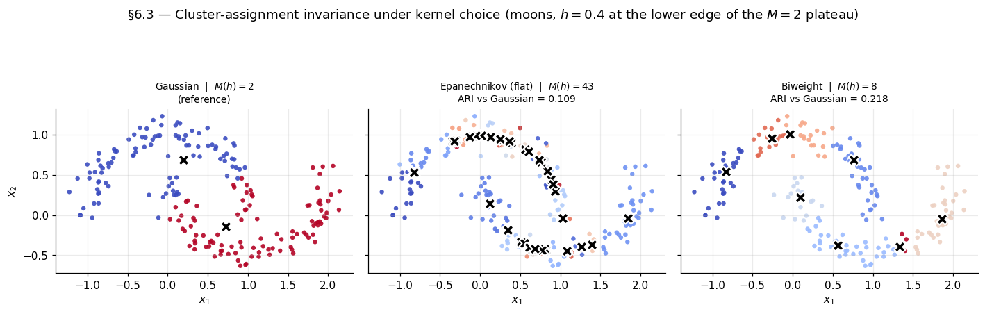
The basin-of-attraction structure is determined by the topology of $\hat f_h$. At bandwidth in the §5 plateau, $\hat f_h$ is locally smoothed enough that the global mode structure is robust to kernel-shape changes. The cluster assignment is invariant up to label permutation across kernel choice.

Two reasons. Smoothing-stable mode count: §5.2’s duality holds for any convex-profile radial kernel; the plateau corresponds to a bandwidth range with stable mode count regardless of small perturbations including kernel shape. Basin-boundary stability: basin boundaries are determined by saddle-ridge structure, stable under the same perturbations. Carreira-Perpiñán (2015, §3.3): “The choice of kernel function has very little effect on the clusters produced by mean-shift, given a sensible bandwidth choice.”

In sharp contrast to KDE-as-density-estimator, where kernel sensitivity at the AMISE-optimal level is real (capped at ~5% by Hodges–Lehmann efficiency). For cluster assignments, sensitivity is essentially zero in the plateau regime.

h (Gaussian; compact kernels scaled ×2): 0.40 dataset:moons3-blob

When kernel choice does matter

Heavy-tailed data, far from the bulk. Gaussian’s exponentially decaying tails give distant points non-zero weight; compact-support kernels give zero. Can shift mode locations near data extremes by amounts crossing cluster boundaries.

Computational cost. Gaussian needs all $n$ data points per query — $O(n)$ per iteration. Compact-support kernels accelerate to $O(\log n + k)$ via kd-tree / ball-tree (§8.3). For large $n$, order-of-magnitude difference.

Smoothness of $\hat f_h$. Gaussian $C^\infty$; Epanechnikov $C^0$; biweight $C^1$; triweight $C^2$. For mean-shift itself it doesn’t matter; for downstream applications using $\hat f_h$ beyond cluster assignment (Hessian estimation, level-set trees), pick a smooth profile.

Recommendation: Gaussian by default; switch to Epanechnikov if computational cost forces it.

---

From trajectories to clusters

§3.5 showed individual trajectories converging. §5.5 used trajectory endpoints as cluster proxies. §7 makes both moves formal.

The trajectory map and basin-of-attraction clustering

Two data points are in the same cluster iff their trajectories converge to the same mode. The map $T_h$ defines a spatial clustering — every point in $\mathbb{R}^d$ has a cluster label, not just the data points. Any new $\mathbf{x}_{\text{new}}$ is classified by running a fresh trajectory.

Basin boundaries are the $(d-1)$-dimensional saddle ridges of $\hat f_h$.

Mode merging with tolerance

In finite precision, two trajectories that should converge to the same mode land at endpoints separated by a small distance. The mode-extraction step needs a merging tolerance $\delta$.

Greedy-union rule (used throughout): walk through endpoints, attach each to an existing mode if within $\delta$, else create a new mode. Heuristics for $\delta$: $\delta \approx 10 \cdot \text{tol}$ (safety margin) or $\delta \approx 0.1 \cdot h$ (well below inter-mode separation). The from-scratch implementation uses $\delta = 10^{-3}$.

The mode-merging tolerance is a numerical parameter, not a clustering hyperparameter; cluster assignment is invariant to $\delta$ over a wide range.

Blurring mean-shift

Cheng (1995, §4) introduces a variant where data points themselves move at each iteration:

$$\mathbf{x}_i^{(t+1)} \;=\; \frac{\sum_j g\bigl(\|(\mathbf{x}_i^{(t)} - \mathbf{x}_j^{(t)})/h\|^2\bigr)\, \mathbf{x}_j^{(t)}}{\sum_j g\bigl(\|(\mathbf{x}_i^{(t)} - \mathbf{x}_j^{(t)})/h\|^2\bigr)}.$$

The KDE is rebuilt at each iteration. Converges much faster — data collapses to modes in geometric time — but Cheng (1995, Theorem 2) shows long-time blurring collapses to a single point regardless of $h$. The practical algorithm runs only a small number of iterations.

Standard (non-blurring) mean-shift is the default: respects the mode-tree structure and the §4 convergence theory.

Initialization

Sample-as-queries — initialize at the data points. Standard for clustering data points.

Grid-as-queries — initialize on a regular grid covering the data extent. Produces the basin-of-attraction map for $\mathbb{R}^d$ (not just the data).

Adaptive initialization — only at “promising” locations (high-$\hat f_h$ regions, coarse-pass modes). For $n \leq 10^4$ in 2D, savings are modest; for very large $n$ in higher $d$, substantial.

The basin-of-attraction map on the moons

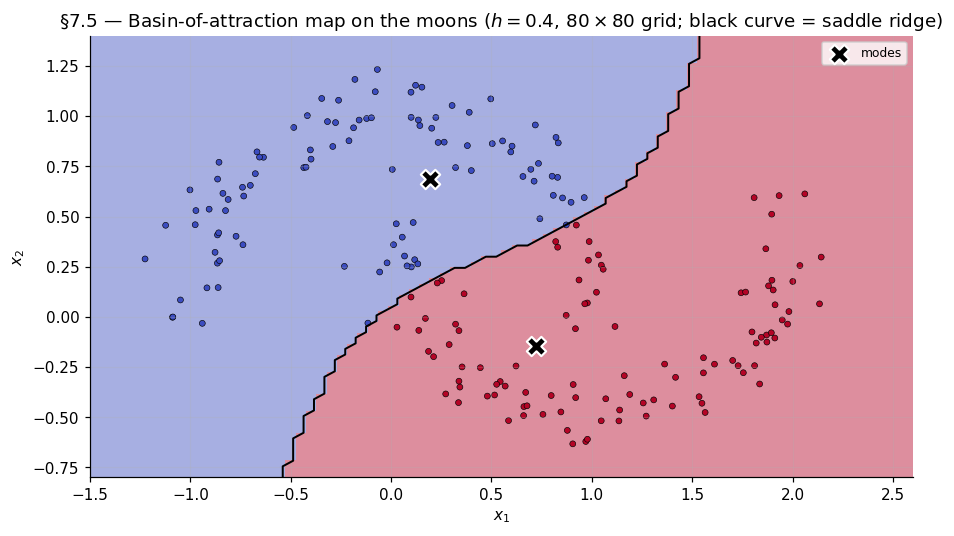
80 × 80 = 6400 trajectories from a grid over the moons range, Gaussian kernel at $h = 0.40$, deduped at tolerance $10^{-3}$. Endpoints aligned to data-trajectory modes for consistent label coloring between basin map and scatter. The basin boundary appears as a smooth curve threading between the two crescents, far from either’s bulk.

---

Practical mean-shift

§§3–7 covered the algorithm and theory. §8 is about what happens when you actually want to run mean-shift on real data.

Design choices in the from-scratch implementation

The mean_shift_trajectories function from §3.5 makes four design choices.

Vectorized pairwise distance. scipy.spatial.distance.cdist for the $m \times n$ squared-distance matrix per iteration — $O(m n)$ in compiled C. Memory $8 m n$ bytes (float64), fine for $m, n \leq 10^4$. At larger scale, batch queries in chunks of $\sim 10^3$.

Log-domain stability. Per-row max-subtract before exponentiating the Gaussian-kernel weights — the subtracted constant cancels in the weighted-mean ratio. Same trick as softmax.

Vectorized convergence. Stop when the maximum per-query step falls below tol. Per-query stopping is more efficient but harder to vectorize.

Full trajectory history returned. $(T+1, m, d)$ array — more memory than necessary if you only need final positions, but needed for diagnostic plots and basin visualizations. At our scale ($T \leq 100$, $m d \leq 10^4$) it’s $\leq 10$ MB.

A production implementation would tighten all four. The notebook implementation is optimized for pedagogical clarity, not throughput.

sklearn.cluster.MeanShift pitfalls

Three quirks worth knowing.

The estimate_bandwidth default. MeanShift() with bandwidth=None calls estimate_bandwidth(X) internally, which is $O(n^2)$ in time and memory. For $n = 10^4$: $10^8$ distance computations, ~800 MB intermediate memory. For $n = 10^5$: $10^{10}$ computations, 80 GB. Always pass an explicit bandwidth=h chosen via §5.4’s selectors.

The internal kernel is flat, not Gaussian. Uses Epanechnikov-shadow update (unweighted mean inside bandwidth ball). Not user-selectable. §6.3 already showed kernel-invariance in the plateau regime; this is rarely a correctness issue but is the source of rare ARI < 1.0 disagreement on boundary points.

Orphan points get label -1. Trajectories not reaching a mode within max_iter (default 300) iterations are labeled -1. Rare at reasonable bandwidth, common at adversarial small $h$.

bin_seeding=True initializes only at coarse-grid bin centers — substantial speedup for large data.

Scaling: kd-tree and ball-tree neighbor queries

For compact-support kernels, only $\mathcal{N}_h(\mathbf{x})$ contributes to $\mathbf{m}_h(\mathbf{x})$. Brute force is $O(n)$ per query; kd-tree (Bentley 1975) or ball-tree (Omohundro 1989) is $O(\log n + k)$ where $k$ is the average neighborhood size. Build time $O(n \log n)$.

At $n = 10^5$ in $\mathbb{R}^2$ with Epanechnikov: brute force $10^{10}$ distance computations per iteration; kd-tree $1.7 \times 10^6$ neighbor lookups. Three orders of magnitude per iteration.

For Gaussian, truncate: ignore $\|\mathbf{x} - \mathbf{x}_i\| > c \cdot h$ for $c \in [3, 4]$ (captures 99.7% of Gaussian mass). Truncated Gaussian admits the same kd-tree acceleration.

scipy.spatial.cKDTree and sklearn.neighbors.BallTree provide tree implementations. Kd-tree for $d \leq 3$; ball-tree for $d \geq 6$; benchmark in between.

The sample-and-cluster pattern

For $n \gg 10^4$, the sample-and-cluster pattern (Carreira-Perpiñán 2015, §6.2) trades small approximation error for order-of-magnitude speedup:

1. Sample $m \ll n$ seed points.
2. Run mean-shift trajectories from seeds; dedupe to mode set.
3. Assign remaining data via nearest-mode kd-tree query.

Total cost $O(m T \log m) + O(n \log m)$. With $m = \sqrt{n}$, dominant term $O(n \log n)$.

Approximation error from sub-sampling: low-density modes may be missed. Harmless for typical clustering; mitigated by stratified sampling for anomaly localization.

Sanity check: from-scratch vs sklearn

Run both implementations on the moons, 3-blob, and 4-blob at plateau bandwidths, with the from-scratch in flat-kernel mode for like-for-like comparison against sklearn’s internal Epanechnikov shadow. Expect mode counts to agree dataset-by-dataset and ARIs in $[0.95, 1.00]$ — small disagreement on boundary points is normal.

---

k-means as the $h \to 0$ Voronoi limit

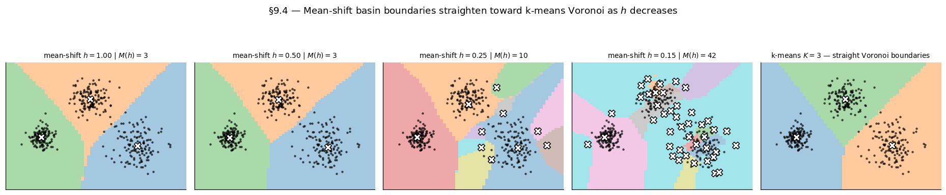
K-means and mean-shift cluster the same data with different parameters and produce different partitions on anything non-Gaussian. §9 makes the relationship precise. Gaussian-kernel mean-shift in the $h \to 0$ limit collapses onto Lloyd’s hard nearest-mean assignment.

Lloyd’s algorithm and the Voronoi-partition fixed point

Lloyd’s algorithm (Lloyd 1982; MacQueen 1967 historical antecedent) picks $K$ centroids (typically via k-means++ seeding, Arthur and Vassilvitskii 2007), then alternates:

1. Assignment. $c(\mathbf{x}_i) = \arg\min_k \|\mathbf{x}_i - \boldsymbol{\mu}_k\|$.
2. Update. $\boldsymbol{\mu}_k \leftarrow (1/|S_k|) \sum_{i \in S_k} \mathbf{x}_i$.

The fixed point locally minimizes the WCSS $J = \sum_k \sum_{i \in S_k} \|\mathbf{x}_i - \boldsymbol{\mu}_k\|^2$. Local convergence; k-means++ providing $O(\log K)$ expected-WCSS approximation.

At a fixed point, $\mathbf{x}_i$ belongs to cluster $k$ iff $\mathbf{x}_i \in V(\boldsymbol{\mu}_k)$ — the Voronoi cell of $\boldsymbol{\mu}_k$. Each cell is a convex polytope; cell boundaries are perpendicular bisectors of centroid pairs.

What each method assumes

K-means. Cluster count $K$ fixed in advance; cluster shape implicitly convex (Voronoi polytope); no density representation. WCSS objective is, up to constants, the NLL of an isotropic Gaussian mixture with equal variances and equal mixing weights (Bishop 2006, §9.1). Works exactly on well-separated isotropic Gaussians. Fails confidently on non-convex / non-isotropic / unequal-spread clusters.

Mean-shift. Cluster count $M(h)$ emerges from $h$; cluster shape is the basin of attraction of $\hat f_h$; density-based. Handles any data with well-defined density modes. Trades $K$ hyperparameter for $h$ hyperparameter.

K-means optimizes WCSS; mean-shift optimizes $\hat f_h$. The silhouette/ARI disagreement on the moons (§1.3) reflects this — silhouette rewards convex compactness (the k-means objective), ARI rewards getting the right partition.

The $h \to 0$ collapse theorem

The convergence rate is exponentially fast in $1/h^2$.

Numerical experiment: ARI(mean-shift, k-means) on the 3-blob

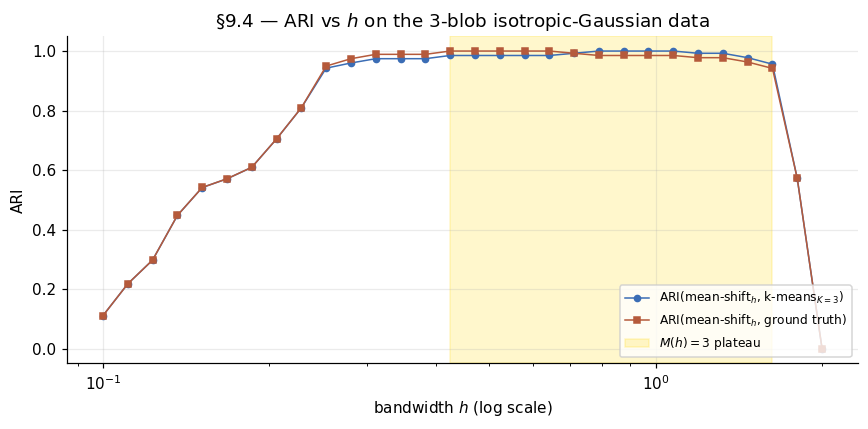
Run k-means with $K = 3$ as reference. Sweep $h$ across the $M(h) = 3$ plateau and below; at each $h$ compute mean-shift labels and ARIs against k-means and against ground truth. ARI(mean-shift, k-means) ≈ 1.0 across the plateau; ARI drops below the plateau when $M(h) > 3$. The basin-mosaic at decreasing $h$ shows boundaries first straightening (within the plateau’s lower edge) then fragmenting (below the plateau).

---

GMM-via-EM and soft assignment

§9 contrasted against k-means — the simplest hard-partition baseline. §10 contrasts against the probabilistic hard-partition baseline: Gaussian mixture models fit by expectation-maximization (Dempster, Laird, and Rubin 1977).

The Gaussian mixture model and its likelihood

$$p(\mathbf{x} \mid \boldsymbol{\theta}) \;=\; \sum_{k=1}^K \pi_k \, \mathcal{N}(\mathbf{x} \mid \boldsymbol{\mu}_k, \boldsymbol{\Sigma}_k),$$

with $\pi_k \geq 0$ summing to 1, component means $\boldsymbol{\mu}_k \in \mathbb{R}^d$, covariances $\boldsymbol{\Sigma}_k \in \mathbb{R}^{d \times d}$ positive definite. Latent-variable form: $z_i \sim \mathrm{Cat}(\boldsymbol{\pi})$, $\mathbf{x}_i \mid z_i = k \sim \mathcal{N}(\boldsymbol{\mu}_k, \boldsymbol{\Sigma}_k)$.

Log-likelihood:

$$\ell(\boldsymbol{\theta}) \;=\; \sum_{i=1}^n \log \sum_{k=1}^K \pi_k\, \mathcal{N}(\mathbf{x}_i \mid \boldsymbol{\mu}_k, \boldsymbol{\Sigma}_k).$$

Log-sum-over-components has no closed-form maximum.

EM for GMMs: responsibilities as soft assignments

E-step. Compute posterior responsibilities:

$$\gamma_{ik}^{(t)} \;:=\; \frac{\pi_k^{(t)}\, \mathcal{N}(\mathbf{x}_i \mid \boldsymbol{\mu}_k^{(t)}, \boldsymbol{\Sigma}_k^{(t)})}{\sum_l \pi_l^{(t)}\, \mathcal{N}(\mathbf{x}_i \mid \boldsymbol{\mu}_l^{(t)}, \boldsymbol{\Sigma}_l^{(t)})}.$$

$\gamma_{ik} \in [0, 1]$ is the soft assignment; $\sum_k \gamma_{ik} = 1$.

M-step. With $N_k = \sum_i \gamma_{ik}^{(t)}$:

$$\pi_k^{(t+1)} = \frac{N_k}{n}, \quad \boldsymbol{\mu}_k^{(t+1)} = \frac{1}{N_k} \sum_i \gamma_{ik}^{(t)}\, \mathbf{x}_i, \quad \boldsymbol{\Sigma}_k^{(t+1)} = \frac{1}{N_k} \sum_i \gamma_{ik}^{(t)}\, (\mathbf{x}_i - \boldsymbol{\mu}_k^{(t+1)})(\mathbf{x}_i - \boldsymbol{\mu}_k^{(t+1)})^\top.$$

Weighted single-Gaussian MLEs. See Bishop (2006, §9.2.2) for the full derivation.

The structural connection to mean-shift: GMM-EM’s M-step $\boldsymbol{\mu}_k = (\sum_i \gamma_{ik} \mathbf{x}_i)/(\sum_i \gamma_{ik})$ is the §3.3 mean-shift update form with responsibilities as kernel weights. Differences: parametric vs fixed-bandwidth weighting; $K$ centroids vs $n$ query points; soft per-component vs hard per-mode. The $h \to 0$ Gaussian-mean-shift → k-means limit (§9.3) and the $\boldsymbol{\Sigma}_k = \sigma^2 \mathbf{I}, \sigma \to 0$ GMM-EM → k-means limit both converge on k-means.

Identifiability, label-switching, and what “the” cluster labels mean

Permuting component labels leaves the density unchanged. The likelihood has $K!$ equivalent global maxima differing only in component naming.

Consequences: EM with random initialization converges to permuted optima; Bayesian inference suffers label-switching (Stephens 2000); cluster-quality metrics must be permutation-invariant (ARI does it, raw accuracy doesn’t).

The label-switching issue affects names, not partition. Two GMM fits agreeing on which samples cluster together but disagreeing on naming are operationally the same fit.

A separate identifiability concern: GMM likelihood is unbounded above. Setting $\boldsymbol{\mu}_k = \mathbf{x}_i$ and $\boldsymbol{\Sigma}_k \to 0$ sends $\ell \to \infty$. sklearn.mixture.GaussianMixture regularizes via reg_covar (default $10^{-6}$).

The M-open critique

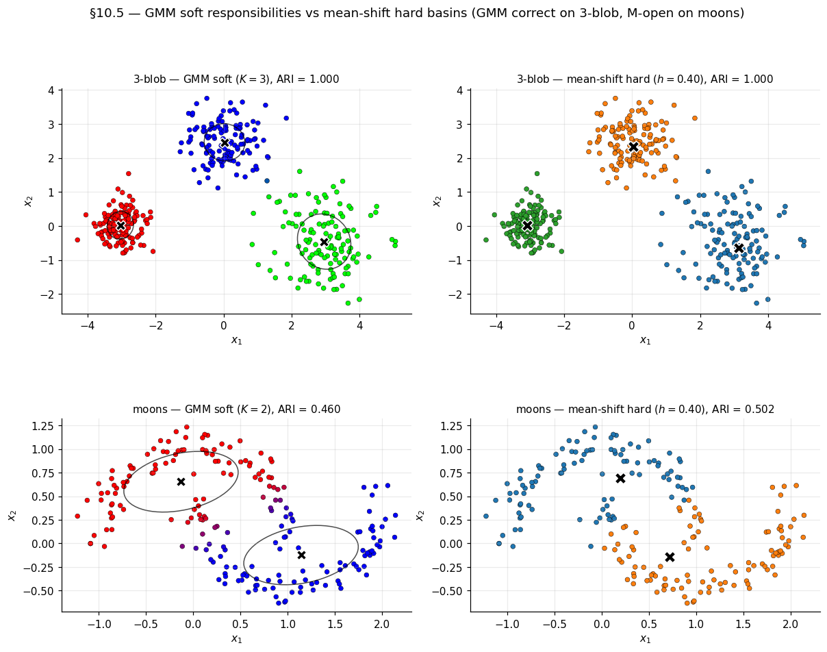
GMM produces correct cluster assignments when data is genuinely a Gaussian mixture. When it isn’t, assignments are systematically biased: GMM fits ellipsoidal components to non-ellipsoidal cluster structure.

Bernardo and Smith (1994) framework: M-closed = true model is in our class; M-complete = known true model is intractable; M-open = true model is outside our class.

For clustering, GMM is M-open whenever cluster shapes aren’t ellipsoidal — most real data. Moons aren’t Gaussian. Concentric rings aren’t. Image segmentation, text embedding, biological data — none are Gaussian in any literal sense.

The critique cuts in two directions. Against GMM: when true clusters are non-Gaussian, biased assignments. Against mean-shift: non-parametric in $\hat f_h$ but commits to “cluster = basin of attraction of kernel-smoothed empirical density.” Less restrictive than ellipsoidal Gaussian, but not assumption-free.

Practical takeaway. Approximately-Gaussian clusters with arbitrary covariance shape: GMM-EM. Non-Gaussian or unknown-shape clusters: mean-shift. On real data, “run both and compare.”

GMM responsibilities vs mean-shift basins

3-blob (where GMM is correct): GMM-EM recovers components; responsibilities sharp inside blobs, soft at boundaries; mean-shift hard MAP agrees up to label permutation; ARI $\approx 1.0$ on both.

Moons (both partially M-open): GMM-EM with $K = 2$ fits two ellipsoids that span across the crescent gap, ARI $\approx 0.46$. Mean-shift at the plateau bandwidth finds the right cluster count and shape but mis-classifies boundary points, ARI $\approx 0.43$. Both algorithms beat k-means’ ARI $\approx 0.22$ from §1.3 but neither recovers the moons perfectly at noise = 0.1 — the crescents are intrinsically hard at this noise level.

K (GMM, 3-blob): 3h (mean-shift, 3-blob; moons uses 0.6h): 0.65 covariance:fulldiagonalsphericaltiedshow ellipses

---

Pointers: spectral and density-based clustering

§§9–10 covered partition-based contrasts. §11 covers two methods that don’t fit cleanly into either partition-based or mode-based — spectral clustering and DBSCAN. Light pointer; proper coverage of spectral clustering is in graph-laplacians and random-walks.

Affinity graphs and the Laplacian

Spectral clustering builds an affinity graph: vertices are samples, edge weights $W_{ij}$ encode pairwise similarity. Standard constructions: Gaussian similarity $W_{ij} = \exp(-\|\mathbf{x}_i - \mathbf{x}_j\|^2 / (2\sigma^2))$; $k$-NN graph; $\epsilon$-graph. $k$-NN is most common: sparse, robust to $\sigma$, density-adaptive.

Graph Laplacian: $L := D - W$, $D = \mathrm{diag}(\sum_j W_{ij})$. Normalized variants: $L_{\mathrm{sym}} := D^{-1/2} L D^{-1/2}$ (Ng–Jordan–Weiss); $L_{\mathrm{rw}} := D^{-1} L$ (Shi–Malik). Eigenvectors corresponding to smallest eigenvalues encode cluster structure: for an ideal $K$-component disconnected graph the bottom $K$ eigenvectors are component indicators; for almost-disconnected graphs they approximately encode the clusters (Mohar 1991; von Luxburg 2007).

Shi–Malik and Ng–Jordan–Weiss

Shi and Malik (2000). Bottom eigenvectors of $L_{\mathrm{rw}}$; for $K = 2$, partition by sign of second-smallest eigenvector; for $K > 2$, recursive bipartitioning or k-means on bottom $K$ eigenvectors. Motivated by the normalized cut objective.

Ng, Jordan, and Weiss (2002). Bottom $K$ eigenvectors of $L_{\mathrm{sym}}$ as $V \in \mathbb{R}^{n \times K}$. Row-normalize: $Y_{ij} = V_{ij}/\sqrt{\sum_l V_{il}^2}$. Run k-means on rows of $Y$. Geometric interpretation: row-normalized embedding lies on the unit sphere in $\mathbb{R}^K$, where cluster structure is spherical.

For the variational characterization, Cheeger inequality, perturbation analysis, random-walk dual — consult graph-laplacians and random-walks. von Luxburg (2007) is the standard intro.

DBSCAN

Density-Based Spatial Clustering of Applications with Noise (Ester, Kriegel, Sander, and Xu 1996). Two hyperparameters: $\epsilon$ (neighborhood radius) and $\text{MinPts}$. Point types: core ($|\mathcal{N}_\epsilon(\mathbf{x}_i)| \geq \text{MinPts}$), border (in a core’s neighborhood, not itself core), noise (neither). Clusters are connected components of density-reachability between core points; noise gets label $-1$.

DBSCAN vs mean-shift: both density-based, but DBSCAN uses hard threshold ($\epsilon$, MinPts) while mean-shift uses KDE smoothing. DBSCAN handles noise via $-1$; mean-shift assigns every point. DBSCAN has 2 hyperparameters, mean-shift 1. HDBSCAN (Campello, Moulavi, Sander 2013) replaces fixed $\epsilon$ with a hierarchy.

For uniform-density clusters, DBSCAN excels. For varied-density data, it struggles — single $\epsilon$ can’t resolve both tight and diffuse clusters; mean-shift’s bandwidth adapts via KDE smoothing.

Numerical demonstration on make_circles

make_circles(n_samples=200, factor=0.5, noise=0.05): outer ring radius 1.0, inner ring radius 0.5. KDE density is concentrated on ring-shaped ridges, not point modes — mean-shift trajectories converge to points along the ridges, basin partition fragments. Spectral and DBSCAN both succeed by exploiting connected-component structure on the affinity graph.

Four panels: mean-shift fails (ARI $\approx 0$); spectral $K = 2$ with $k = 10$-NN affinity succeeds (ARI $\approx 1$); DBSCAN $\epsilon = 0.20$ MinPts $= 5$ succeeds (ARI $\approx 1$); spectral embedding showing linear separability of the two rings.

Light pointer per §11. Full spectral-clustering theory lives in graph-laplacians and random-walks in the Graph Theory track.

h (mean-shift): 0.20 K (spectral): 2kNN (affinity): 10ε (DBSCAN): 0.20

---

Connections, limits, and forward pointers

Within-formalML siblings

Kernel regression (Supervised Learning, intermediate). Covariate-conditional KDE counterpart. The NW estimator is structurally identical to Gaussian-kernel mean-shift update; kernel regression averages responses, mean-shift averages positions; same machinery.

Graph Laplacians (Graph Theory, advanced). Proper home for spectral clustering — eigenvalue spectrum, Cheeger inequality, perturbation analysis. §11 gestures; graph-laplacians develops.

Random walks (Graph Theory, intermediate). Dual Laplacian view: $L_{\mathrm{rw}}$ generates a random walk; mixing times encoded by spectral eigenvalues.

Normalizing flows (Unsupervised, advanced). Continuous-density estimation via invertible neural transformations. Mean-shift’s KDE is the non-parametric precursor to flow-based estimators.

Forward pointers

Density-ratio estimation (coming soon). KLIEP, LSIF, uLSIF — density-ratio estimators that plug KDE substrates into $r(\mathbf{x}) = p_{\text{num}}/p_{\text{den}}$. The unsupervised.ts exports meanShift and modeFinder are direct dependencies. Closes the T3 Unsupervised track.

Honest limits

Curse of dimensionality on $h$. AMISE-optimal $h^* \asymp n^{-1/(d+4)}$ grows with $d$, but the bandwidth-ball volume grows much faster — $|B(\mathbf{x}, h)| \propto h^d$. In $d = 10$ with $n = 10^3$, the typical neighborhood at $h^*$ contains essentially zero samples. Mean-shift becomes infeasible above $d \approx 10$ without dimensionality reduction (PCA, autoencoder, t-SNE / UMAP) as preprocessing.

Mode-vs-cluster distinction. Mean-shift converges to stationary points; the modal-clustering hypothesis (Hartigan 1975) asserts cluster = basin of attraction of a density mode. Three failure modes: well-separated clusters that don’t produce distinct density modes (concentric rings); spurious modes from noise; genuinely ambiguous cluster structure where no algorithm agrees.

No cluster-count guarantees under noise. Under additive noise, KDE develops spurious local maxima counting toward $M(h)$. The bandwidth-mode-count duality is preserved (still monotone) but the plateau may shift or disappear. Carreira-Perpiñán (2015, §3.3) discusses noise-robust mode estimation; practical fix is to combine moderate bandwidth with a low-density-prune step dropping modes with insufficient basin mass.

Take-home. Mean-shift is the right tool for cluster discovery via density modes on moderate-dimensional, moderately-noised data with moderately-distinct cluster shapes. Outside that regime, k-means, GMM, spectral, DBSCAN are alternatives — on hard data, ensembles often do better than any single one.