Random Walks & Mixing
Markov chains on graphs — from the transition matrix to mixing times, hitting times, and the spectral gap
Overview & Motivation
In the Graph Laplacians & Spectrum topic, we studied graphs through the lens of the Laplacian matrix and its eigenvalues. The normalized Laplacian made a brief appearance alongside the transition matrix . Now we place center stage.
A random walk on a graph is the simplest possible stochastic process on a network: at each step, the walker moves to a uniformly random neighbor. Despite this simplicity, the walk’s behavior reveals deep structural properties:
-
How quickly does the walk forget its starting position? The mixing time measures convergence to the stationary distribution. Fast mixing implies good connectivity — the graph has no bottlenecks.
-
How far apart are two vertices in “random walk distance”? The hitting time measures the expected number of steps to reach from . Unlike shortest-path distance, hitting time is sensitive to the graph’s branching structure and reflects the “difficulty” of finding a target by random exploration.
-
What is the electrical interpretation? Identifying edges with unit resistors turns the graph into an electrical network. The effective resistance between two vertices equals the commute time (normalized by total edge weight) — a beautiful equivalence between probability and physics.
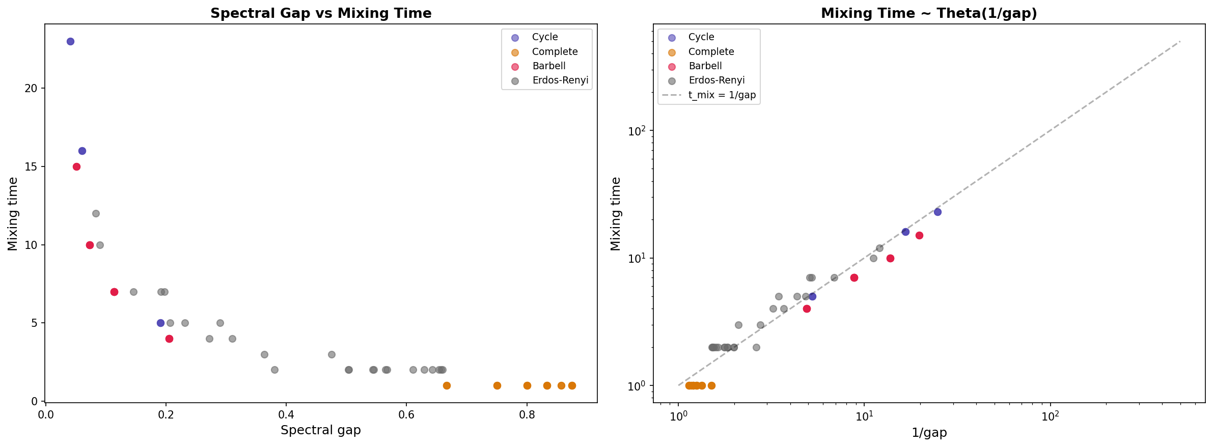
The spectral gap is the key quantity: it controls mixing time (), bounds hitting times, and characterizes Expander Graphs — sparse graphs that mix as fast as dense ones.
Roadmap. We build the theory in layers: define the walk and its transition matrix (§1), prove convergence to the stationary distribution (§2), quantify convergence speed via total variation and mixing time (§3–4), handle bipartite graphs with lazy walks (§5), develop hitting times and commute times (§6–7), and connect everything to applications (§8–9).
1. Markov Chains on Graphs
1.1 The Transition Matrix
A random walk on a graph with is a sequence of random variables taking values in , where at each step the walker moves to a uniformly random neighbor:
Definition 1 (Random Walk on a Graph).
A random walk on a graph is a Markov chain on the state space with transition probabilities : at each step, the walker moves from its current vertex to a uniformly random neighbor.
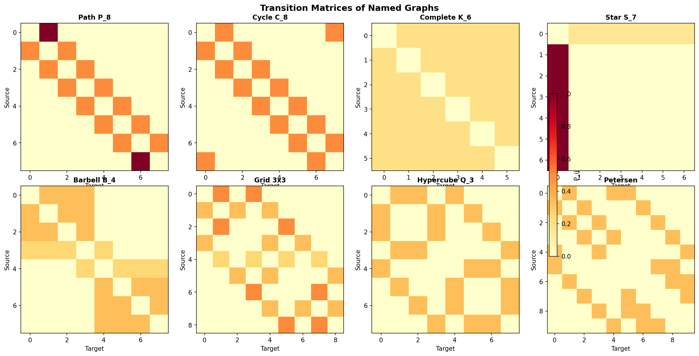
Definition 2 (Transition Matrix).
The transition matrix of the simple random walk on is:
where is the degree matrix. Each row of sums to 1 — is a (row) stochastic matrix.
The entry gives the probability of stepping from vertex to vertex in one step. The matrix gives -step transition probabilities: .
1.2 Irreducibility and Aperiodicity
Two properties determine the walk’s long-run behavior:
- Irreducible: Every vertex can be reached from every other vertex (equivalently, is connected).
- Aperiodic: The walk does not get trapped in a deterministic cycle. A connected graph has period 2 if and only if it is bipartite. All other connected graphs are aperiodic.
Combining these:
Definition 3 (Ergodic Chain).
A Markov chain is ergodic if it is both irreducible and aperiodic. For graph random walks, this means is connected and non-bipartite.
2. Stationary Distribution & Convergence
2.1 The Stationary Distribution
Definition 4 (Stationary Distribution).
A probability distribution is stationary for if . Equivalently, if the walk’s initial distribution is , it remains after any number of steps.
Theorem 1 (Stationarity of π).
The stationary distribution of the simple random walk on is where .
Proof.
We verify directly:
The degree in the numerator cancels, and since the column sum of the adjacency matrix equals the degree of vertex .
∎The stationary distribution assigns probability proportional to degree. High-degree vertices are visited more often — they are “easier to find” because more edges lead to them. On a -regular graph, all degrees are equal and — the uniform distribution.
Corollary 1 (Mixing of Regular Graphs).
On a -regular graph, the stationary distribution is uniform: .
2.2 Detailed Balance (Reversibility)
Theorem 2 (Detailed Balance (Reversibility)).
The simple random walk on any undirected graph is reversible: for all .
Proof.
The equality follows from the graph being undirected.
∎Remark (Reversibility and the Inner Product).
Detailed balance means the walk is time-reversible: a video of the walk looks the same played forwards and backwards (in distribution). Algebraically, reversibility is equivalent to being self-adjoint with respect to the inner product .
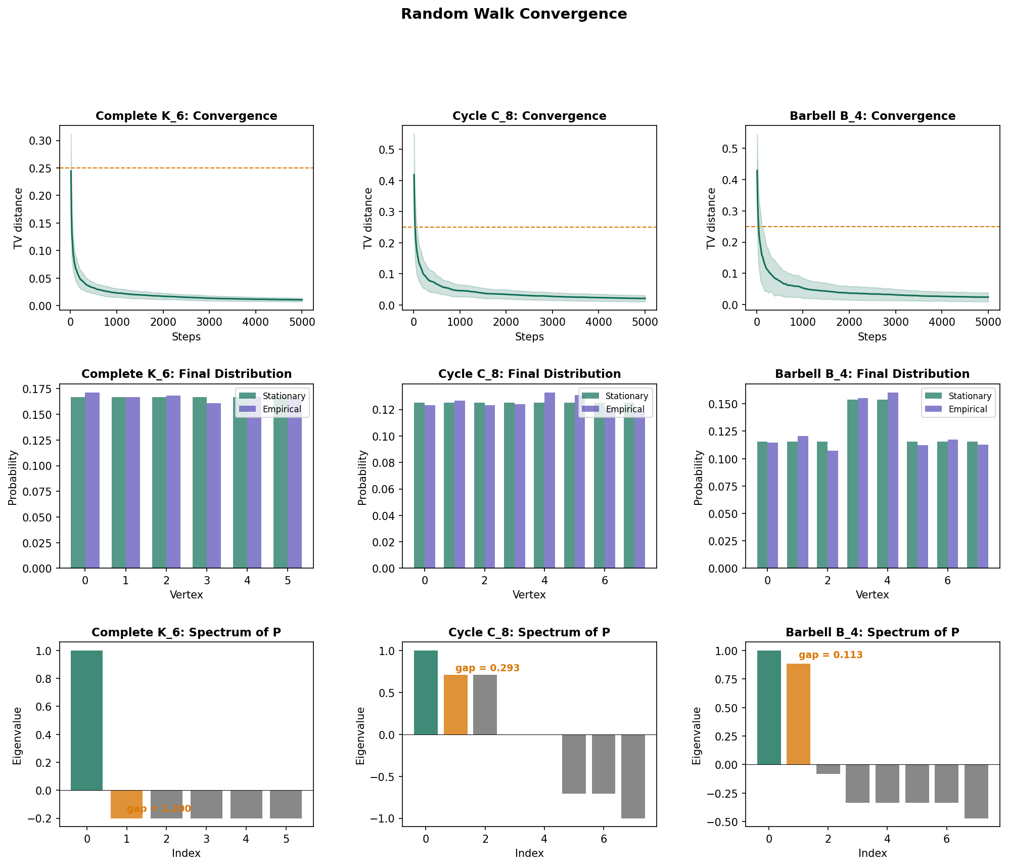
2.3 Convergence
Theorem 3 (Convergence Theorem).
If the random walk on is ergodic (connected, non-bipartite), then for any starting vertex :
Proof.
By the Perron–Frobenius theorem applied to the non-negative irreducible matrix : the largest eigenvalue is simple (by irreducibility), and aperiodicity ensures for all .
The spectral decomposition gives:
Since , each term as , so . That is, every row of converges to .
∎
3. Total Variation & Mixing Time
The convergence theorem says the walk eventually reaches stationarity, but how fast? We need a distance measure between distributions.
Definition 5 (Total Variation Distance).
The total variation distance between probability distributions and on is:
Total variation ranges from 0 (identical distributions) to 1 (distributions with disjoint support). It has a clean probabilistic interpretation: — the maximum difference in probability assigned to any event.
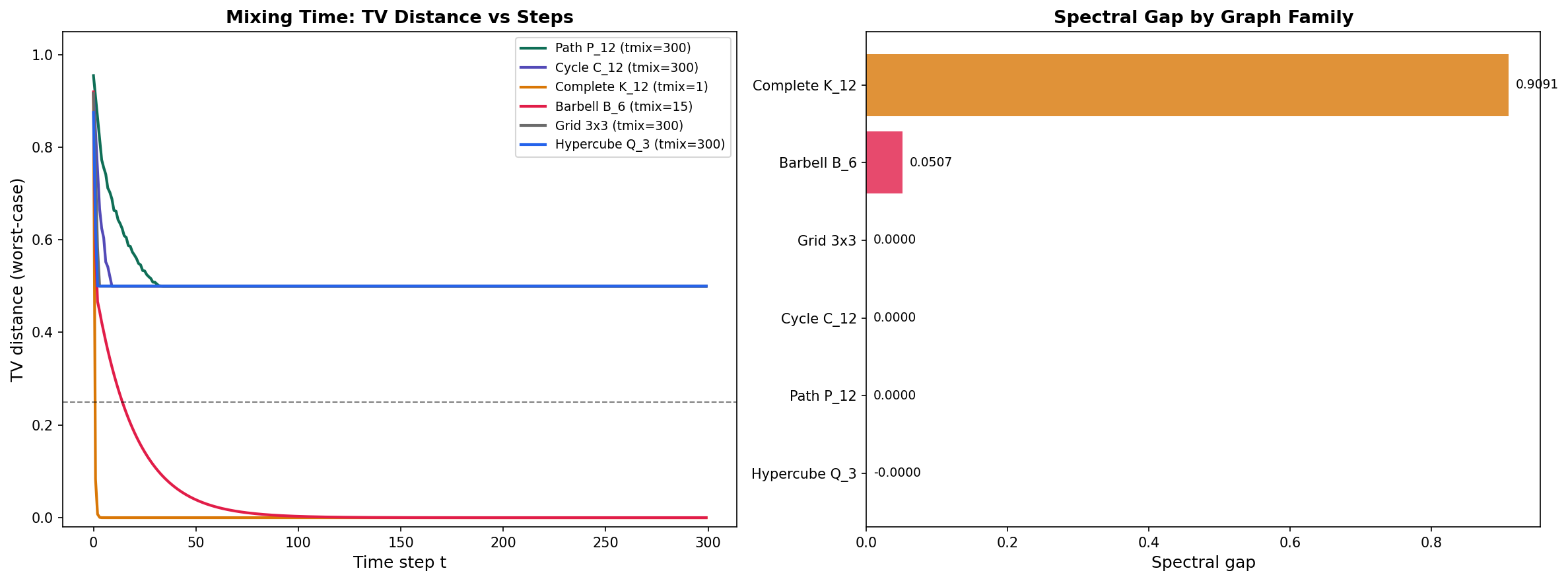
Definition 6 (Mixing Time).
The mixing time to accuracy is the worst-case time for the walk to get -close to stationarity:
By convention, .
Examples illustrating the range of mixing behaviors:
- Complete graph : . Every vertex is adjacent to every other — the walk mixes in a single step.
- Cycle : . The walk must diffuse around the ring.
- Path : . Similar to the cycle, but without the wraparound.
- Barbell : . The bridge is a bottleneck — the walk gets stuck in one clique.
- Hypercube : . Fast mixing despite sparsity — each vertex has degree out of vertices.
4. Spectral Analysis of Mixing
4.1 Spectral Decomposition of
Theorem 4 (Spectral Decomposition of P^t).
Let be the eigenvalues of , with corresponding right eigenvectors (normalized in ). Then:
Proof.
Since is similar to the symmetric matrix (via the Spectral Theorem), it has real eigenvalues and a complete eigenbasis. Write in the spectral decomposition:
where and are right and left eigenvectors. The term is (since and ). For ergodic chains, for , so each remaining term decays exponentially.
∎The rate of decay is controlled by , the second-largest eigenvalue in absolute value. This leads to:
4.2 The Spectral Gap
Definition 7 (Spectral Gap).
The spectral gap of the random walk is:
Corollary 2 (Spectral Gap Equals λ₂(𝓛)).
For non-bipartite graphs, and the spectral gap equals the second-smallest eigenvalue of the normalized Laplacian: .
This is the bridge between random walks and spectral graph theory: the same eigenvalue that measures algebraic connectivity in the Laplacian world controls mixing speed in the random walk world.
4.3 Mixing Time Bounds
Theorem 5 (Upper Mixing Time Bound).
Proof.
Apply Cauchy–Schwarz in . The total variation distance satisfies:
The norm of is bounded by using the spectral decomposition.
∎This gives the mixing time bound: .
Theorem 6 (Lower Mixing Time Bound).
Proof.
Consider the second eigenvector test function. For the worst-case starting vertex, the TV distance at time is at least . Setting this equal to and solving for gives the lower bound.
∎Summary: . The spectral gap is the dominant factor; the term accounts for graphs with extreme degree variation.
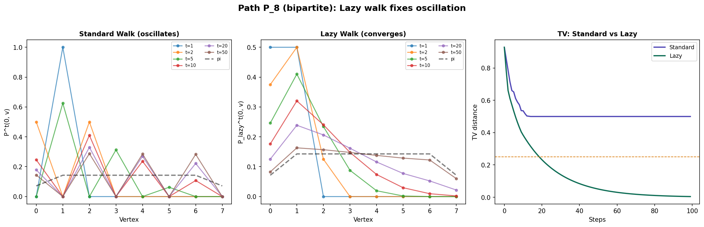
5. Lazy Random Walks
What happens on bipartite graphs? The path graph and the grid graph are bipartite, so has eigenvalue and the walk oscillates instead of converging. The distribution at even time steps differs from odd time steps. The fix is simple:
Definition 8 (Lazy Random Walk).
The lazy random walk has transition matrix:
At each step, the walker stays put with probability and moves to a random neighbor with probability .
Proposition 1 (Lazy Walk Spectrum).
If are eigenvalues of , then the eigenvalues of are .
Proof.
If , then:
So is an eigenvector of with eigenvalue .
∎Since , we have — no negative eigenvalues, no oscillation. The lazy walk converges even on bipartite graphs, at the cost of halving the spectral gap: .
6. Hitting Times & Commute Times
Mixing time measures convergence of the distribution to stationarity. Hitting times measure something complementary: how long it takes a single walk to reach a specific target.
Definition 9 (Hitting Time).
The hitting time from to is the expected first passage time:
with by convention.
Hitting times satisfy a linear recurrence: for .
Proposition 2 (Hitting Time via Fundamental Matrix).
For each target , the hitting times satisfy the linear system:
where is the transition matrix with row and column removed.
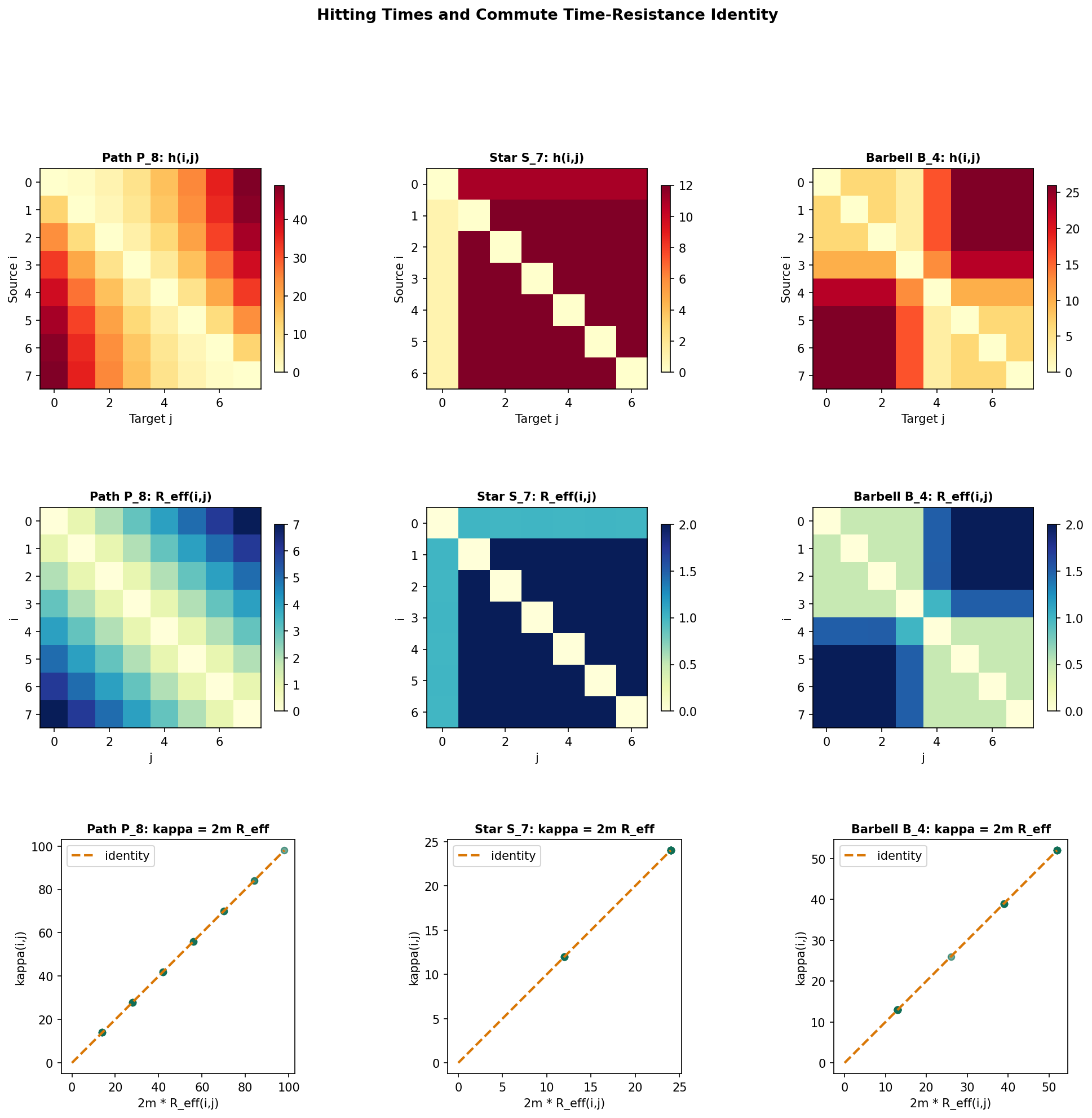
Hitting times are asymmetric in general: . On a star graph with 1 hub and leaves, any leaf reaches the hub in exactly 1 step (), but the hub must guess the right leaf: . To go from one leaf to another, the walker first steps to the hub (1 step) then searches for the target leaf ( steps on average), giving . The asymmetry reflects the graph’s branching structure.
Definition 10 (Commute Time).
The commute time between and is the expected round-trip time:
Unlike hitting times, commute times are symmetric: .
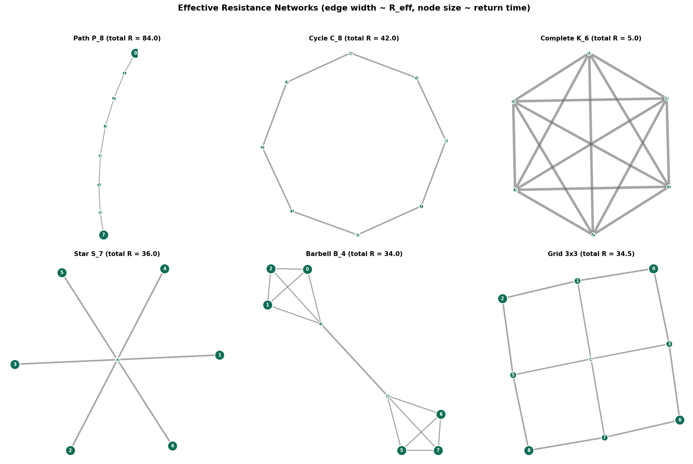
7. Effective Resistance & Electrical Networks
The connection between random walks and electrical networks is one of the most beautiful results in combinatorics. Replace each edge with a unit resistor, and the graph becomes an electrical circuit. The Laplacian is the conductance matrix: applying Kirchhoff’s laws gives .
Definition 11 (Effective Resistance).
The effective resistance between vertices and is:
where is the Moore–Penrose pseudoinverse of the Laplacian and is the -th standard basis vector.
Effective resistance is a metric on : it satisfies non-negativity, symmetry, and the triangle inequality. It behaves like physical resistance — adding edges decreases resistance (parallel paths), removing edges increases it.
Theorem 7 (Commute Time–Effective Resistance Identity).
where is the total number of edges.
Proof.
Express via the fundamental matrix : we have . Adding and using (after appropriate normalization), the entries telescope to give .
See Doyle & Snell (1984) for the complete derivation.
∎Properties of effective resistance:
- with equality if and only if .
- Symmetric: .
- Triangle inequality: .
- Rayleigh monotonicity: Adding edges can only decrease effective resistance.
Random Target Lemma: .
8. Applications: PageRank, DeepWalk, Label Propagation
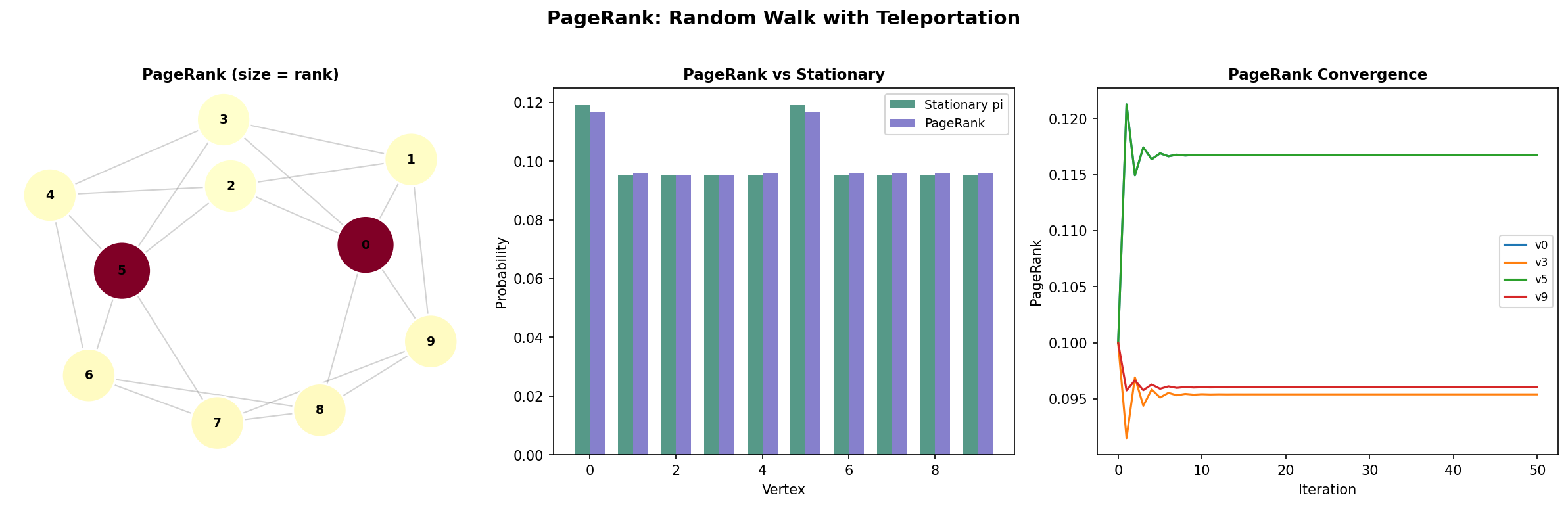
8.1 PageRank
PageRank (Page, Brin, Motwani & Winograd, 1999) models a web surfer who follows links randomly, but occasionally “teleports” to a uniformly random page:
with typically. The teleportation term is a rank-one perturbation that guarantees ergodicity — even if the original graph is disconnected or bipartite.
Remark (PageRank as Perturbed Random Walk).
The teleportation term guarantees a spectral gap of at least , so PageRank converges in iterations regardless of graph structure. This is why power iteration converges fast for PageRank — the teleportation creates an artificial spectral gap.
8.2 DeepWalk and node2vec
DeepWalk (Perozzi, Al-Rfou & Skiena, 2014) treats random walks as “sentences” and vertices as “words,” then applies the skip-gram model from NLP to learn vertex embeddings. The key insight: DeepWalk implicitly factorizes a matrix related to , connecting random walk statistics to low-rank matrix approximations studied in PCA & Low-Rank Approximation.
8.3 Label Propagation
Label propagation spreads known labels through the graph:
At convergence, each vertex’s label is a discounted average of its neighbors’ labels, weighted by the random walk transition probabilities. The mixing time determines how far labels spread — fast-mixing graphs propagate labels globally, while graphs with bottlenecks propagate locally.
Remark (Over-Smoothing in GNNs).
Stacking GCN layers applies to the feature matrix. By the convergence theorem, — all vertex features collapse to a single vector. This is over-smoothing: the random walk convergence theorem in disguise. The number of useful GNN layers should roughly match , the mixing time. Message Passing & GNNs develops solutions to this problem.
9. Computational Notes
Transition matrix construction. Given an adjacency matrix (as a NumPy array or scipy sparse matrix), the transition matrix is :
import numpy as np

def transition_matrix(A):
    """P = D^{-1}A for simple random walk."""
    D_inv = np.diag(1.0 / A.sum(axis=1))
    return D_inv @ A
Random walk simulation. Simulate a walk and track visit frequencies:
def simulate_walk(P, start, n_steps, rng=None):
    """Simulate a random walk, return visit counts."""
    rng = rng or np.random.default_rng()
    n = len(P)
    counts = np.zeros(n)
    v = start
    for _ in range(n_steps):
        counts[v] += 1
        v = rng.choice(n, p=P[v])
    return counts / n_steps
Mixing time estimation via spectral decomposition. Compute TV distance at each step without matrix exponentiation:
def mixing_profile(A, max_t=200):
    """TV distance at each step via spectral decomposition."""
    P = transition_matrix(A)
    deg = A.sum(axis=1)
    deg = np.where(deg == 0, 1, deg)  # guard against isolated vertices
    pi = deg / deg.sum()
    inv_sqrt_deg = 1.0 / np.sqrt(deg)
    evals, evecs = np.linalg.eigh(
        np.diag(inv_sqrt_deg) @ A @ np.diag(inv_sqrt_deg)
    )
    # evals of S = D^{-1/2}AD^{-1/2} equal evals of P
    tv = []
    for t in range(max_t + 1):
        max_tv = 0
        for x in range(len(A)):
            dist = np.zeros(len(A))
            for k in range(len(A)):
                dist += evals[k]**t * evecs[:, k] * evecs[x, k]
            dist = dist * np.sqrt(A.sum(axis=1)) / np.sqrt(A.sum(axis=1)[x])
            max_tv = max(max_tv, 0.5 * np.sum(np.abs(dist - pi)))
        tv.append(max_tv)
    return tv
Hitting time solver. Solve the linear system for all-pairs hitting times:
def all_pairs_hitting_times(A):
    """Solve (I - P_{-j}) h_j = 1 for each target j."""
    P = transition_matrix(A)
    n = len(A)
    H = np.zeros((n, n))
    for j in range(n):
        idx = [i for i in range(n) if i != j]
        P_red = P[np.ix_(idx, idx)]
        h = np.linalg.solve(np.eye(n-1) - P_red, np.ones(n-1))
        for k, i in enumerate(idx):
            H[i, j] = h[k]
    return H
Effective resistance. Compute via the Laplacian pseudoinverse:
def effective_resistance_matrix(A):
    """R_eff(i,j) via Laplacian pseudoinverse."""
    L = np.diag(A.sum(axis=1)) - A
    evals, evecs = np.linalg.eigh(L)
    # Pseudoinverse: invert nonzero eigenvalues
    L_pinv = sum(
        (1/lam) * np.outer(v, v)
        for lam, v in zip(evals, evecs.T) if lam > 1e-10
    )
    R = np.zeros_like(A, dtype=float)
    for i in range(len(A)):
        for j in range(i+1, len(A)):
            R[i,j] = R[j,i] = L_pinv[i,i] + L_pinv[j,j] - 2*L_pinv[i,j]
    return R
PageRank via power iteration. The standard implementation using networkx:
import networkx as nx

G = nx.karate_club_graph()
pr = nx.pagerank(G, alpha=0.85)

# Manual power iteration
A = nx.to_numpy_array(G)
P = transition_matrix(A)
n = len(A)
alpha = 0.85
P_pr = alpha * P + (1 - alpha) / n * np.ones((n, n))
r = np.ones(n) / n
for _ in range(100):
    r = r @ P_pr
10. Connections & Further Reading
Cross-Track and Within-Track Connections
| Topic | Connection |
|---|---|
| Graph Laplacians & Spectrum | complements . The spectral gap controls both algebraic connectivity and mixing time. |
| The Spectral Theorem | is similar to the symmetric matrix . The spectral decomposition of underlies every mixing bound. |
| Shannon Entropy & Mutual Information | decreases monotonically along the walk. The stationary entropy if and only if the graph is regular. |
| Measure-Theoretic Probability | Convergence in total variation = convergence in on the probability simplex. The ergodic theorem says time averages converge almost surely. |
| Concentration Inequalities | Chernoff bounds for sums along a Markov chain use the spectral gap to account for dependence between consecutive samples. |
| PCA & Low-Rank Approximation | DeepWalk/node2vec embeddings implicitly factorize random walk probabilities — a spectral approximation related to Laplacian eigenvectors. |
| Expander Graphs | Expander Graphs are the sparse graphs that mix the fastest — their spectral gap is bounded away from zero even as , giving mixing time. The expander walk sampling theorem extends the mixing perspective to derandomization. |
| Message Passing & GNNs | Over-smoothing in GNNs is the convergence theorem applied to feature propagation: layers ≈ , and collapses features. GNN depth should respect the mixing time. |
Key Notation
| Symbol | Name | Definition |
|---|---|---|
| Transition matrix | ||
| Stationary distribution | ||
| Spectral gap | ||
| Mixing time | Worst-case TV convergence to | |
| Lazy walk | ||
| Hitting time | Expected first passage time | |
| Commute time | ||
| Effective resistance |
Connections
- The transition matrix P = D⁻¹A is the complement of the random walk Laplacian L_rw = I − P. The eigenvalues of P are μᵢ = 1 − λᵢ(L_rw), so the spectral gap of the walk equals the algebraic connectivity λ₂ of the normalized Laplacian. graph-laplacians
- P is similar to D^{1/2} P D^{-1/2} = D^{-1/2} A D^{-1/2}, a real symmetric matrix. The Spectral Theorem guarantees real eigenvalues in [−1, 1] and an orthonormal eigenbasis, which underlies the spectral decomposition of P^t. spectral-theorem
- A random walk defines a sequence of random variables on the vertex set. Convergence in total variation is convergence in the L¹ norm on the probability simplex — a measure-theoretic statement about the walk's law. measure-theoretic-probability
- The KL divergence D_KL(P^t(x,·) ∥ π) decreases monotonically along the walk and reaches zero at stationarity. The stationary entropy H(π) = log n for regular graphs — maximum randomness. The spectral gap controls the rate of entropy production. shannon-entropy
- Chernoff-type bounds for sums of random variables along a Markov chain use the spectral gap to account for dependence — the walk mixes fast enough that consecutive samples are nearly independent. concentration-inequalities
- DeepWalk and node2vec learn vertex embeddings by running random walks and applying skip-gram (implicit low-rank matrix factorization). The embedding captures the random walk transition probabilities — a spectral approximation related to the Laplacian eigenvectors. pca-low-rank
References & Further Reading
- book Markov Chains and Mixing Times — Levin, Peres & Wilmer (2009) The standard textbook — covers mixing times, spectral methods, coupling, and hitting times with full proofs
- book Spectral Graph Theory — Chung (1997) Chapter 2 covers random walks on graphs and the connection between mixing and the normalized Laplacian spectrum
- paper The PageRank Citation Ranking: Bringing Order to the Web — Page, Brin, Motwani & Winograd (1999) PageRank = stationary distribution of a random walk with teleportation — the foundational application
- paper DeepWalk: Online Learning of Social Representations — Perozzi, Al-Rfou & Skiena (2014) Random walks for vertex embedding — the bridge from Markov chains to representation learning
- paper Faster Mixing via Average Conductance — Lovász & Kannan (1999) Sharper mixing time bounds via average conductance — extends Cheeger's inequality to the random walk setting
- book Random Walks and Electric Networks — Doyle & Snell (1984) The classic treatment of the equivalence between random walk quantities and electrical network quantities