Expander Graphs

Overview & Motivation

The complete graph $K_n$ is well-connected in every sense: every pair of vertices shares an edge, every subset has a massive boundary, and a random walk mixes in a single step. But $K_n$ has $\binom{n}{2}$ edges — a quadratic cost that becomes prohibitive for large $n$. Can we achieve the same qualitative connectivity with far fewer edges?

Expander graphs say yes. An expander is a graph that is simultaneously sparse (each vertex has bounded degree $d$, independent of $n$, so the total edge count is $O(n)$) and well-connected (every vertex subset $S$ with $|S| \leq n/2$ has a boundary at least proportional to $|S|$). This combination sounds paradoxical: how can a graph with only $O(n)$ edges avoid having bottlenecks? And yet expander families exist, can be constructed explicitly, and turn out to be optimal in a precise spectral sense.

Three equivalent perspectives capture the “no bottleneck” property:

1. Vertex expansion: Every set $S$ has many neighbors outside $S$ — the boundary $N(S) \setminus S$ is large relative to $|S|$.

2. Edge expansion (the Cheeger constant): Every set $S$ has many edges crossing to the complement $\bar{S}$ — the edge boundary $|E(S, \bar{S})|$ is large relative to $|S|$.

3. Spectral expansion: The second-largest eigenvalue $\lambda$ of the adjacency matrix (in absolute value) is bounded away from the degree $d$ — the spectral gap $d - \lambda$ is large.

Cheeger’s inequality links perspectives 2 and 3, showing they are quantitatively equivalent. The Expander Mixing Lemma makes expansion concrete: it controls the number of edges between any two vertex subsets in terms of $\lambda$, making the $(n, d, \lambda)$-expander formalism a workhorse for combinatorics and computer science. The Alon-Boppana bound establishes $\lambda \geq 2\sqrt{d-1} - o(1)$ as a universal floor, and Ramanujan graphs — which achieve $\lambda \leq 2\sqrt{d-1}$ — are the provably optimal expanders.

These results connect directly to the spectral theory we developed in the prerequisite topics. In Graph Laplacians & Spectrum, Cheeger’s inequality linked the Fiedler value $\lambda_2(L)$ to the minimum edge cut. In Random Walks & Mixing, the spectral gap $\gamma = 1 - \lambda_2(P)$ controlled the mixing time. Expanders are the graphs where both quantities are bounded away from zero uniformly in $n$ — the mixing time is $O(\log n)$ regardless of the graph’s size, and the minimum cut grows linearly with the subset size.

Why should ML practitioners care? Expanders appear throughout theoretical computer science and increasingly in machine learning:

• Derandomization: The expander walk sampling theorem shows that a random walk on an expander produces nearly independent samples, reducing the randomness needed by algorithms from $O(t \log n)$ to $O(\log n + t \log d)$ bits.
• Error-correcting codes: Bipartite expanders yield linear-time decodable codes (Sipser-Spielman expander codes).
• Network design: Communication networks, sensor networks, and distributed systems benefit from expander-like connectivity.
• Graph neural networks: Expansion controls information flow in message-passing architectures — $O(\log n)$ layers suffice to propagate information across the entire graph, but also cause over-smoothing.

Roadmap. We define the three expansion notions and compute them on named graphs (§1-2), prove their equivalence via Cheeger’s inequality (§3), derive the Expander Mixing Lemma with a full spectral proof (§4), establish the Alon-Boppana lower bound and define Ramanujan graphs (§5), construct explicit expanders from Cayley graphs and number theory (§6), prove the $O(\log n)$ mixing time bound (§7), and survey applications to CS and ML (§8-9).

---

1. Three Notions of Expansion

The central idea of expansion is that every small-to-medium vertex subset has a large boundary. Different notions formalize “boundary” differently. We will define all three, compute them on familiar graphs, and then prove they are equivalent for families of regular graphs.

1.1 Vertex Expansion

The most direct notion counts how many new vertices a set $S$ can reach in one step.

A graph has good vertex expansion if $h_V(G) \geq c$ for some constant $c > 0$ independent of $n$. This means every set $S$ of size at most $n/2$ has at least $c|S|$ neighbors outside $S$ — the graph has no isolated clusters.

1.2 Edge Expansion (the Cheeger Constant)

Instead of counting boundary vertices, we can count boundary edges.

The Cheeger constant measures the minimum “surface-to-volume ratio” of any subset — a direct analogy with isoperimetric inequalities in geometry. A set with small edge boundary relative to its volume is a bottleneck: information (or random walkers) trapped inside $S$ must pass through a narrow gate to reach $\bar{S}$. Expanders are graphs with no such bottlenecks.

1.3 Spectral Expansion

The third perspective replaces the combinatorial min over subsets with a single algebraic quantity: the second-largest eigenvalue.

The quantity $\lambda(G)$ is the largest eigenvalue in absolute value after the trivial eigenvalue $d$. The smaller $\lambda$ is, the better the expansion: the gap between $d$ and $\lambda$ — the spectral gap $d - \lambda$ — measures how far the graph’s spectrum deviates from the rank-1 pattern of the complete graph.

Why does the spectral gap control expansion? Recall from Graph Laplacians & Spectrum that the Laplacian eigenvalues $\mu_i$ of a $d$-regular graph satisfy $\mu_i = d - \lambda_i(A)$. So $\lambda_2(L) = d - \lambda_2(A)$, and a large spectral gap in $A$ means a large Fiedler value $\lambda_2(L)$ — the graph is hard to cut. The connection to Random Walks & Mixing is equally direct: the transition matrix $P = A/d$ has eigenvalues $\lambda_i(P) = \lambda_i(A)/d$, so the spectral gap of the walk is $\gamma = 1 - \lambda(G)/d$.

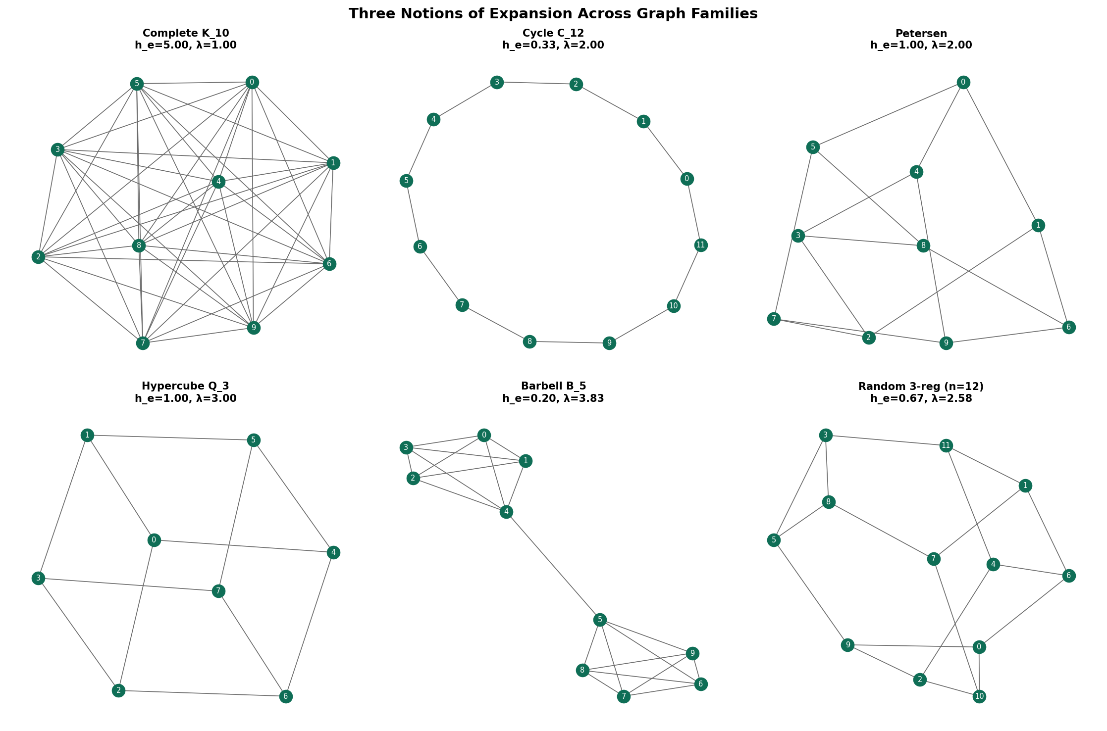
1.4 Examples: Expansion on Named Graphs

Let us compute all three expansion parameters for familiar graphs.

Complete graph $K_n$ ($d = n-1$). Every vertex is adjacent to every other, so for any $S$ with $|S| = k \leq n/2$:

• $\partial_V(S) = V \setminus S$, giving $h_V(K_n) = (n-k)/k \geq 1$.
• $|E(S, \bar{S})| = k(n-k)$, giving $h(K_n) = n - k \geq n/2$.
• The adjacency eigenvalues are $n-1$ (once) and $-1$ (with multiplicity $n-1$), so $\lambda(K_n) = 1$.

$K_n$ is an excellent expander spectrally ($\lambda = 1 \ll d = n-1$), but it is not sparse — the degree grows with $n$.

Cycle $C_n$ ($d = 2$). The cycle is a 2-regular graph. Taking $S$ to be a contiguous arc of $\lfloor n/2 \rfloor$ vertices:

• $|\partial_V(S)| = 2$ (the two endpoints of the arc), so $h_V(C_n) = 2/\lfloor n/2 \rfloor \to 0$.
• $|E(S, \bar{S})| = 2$, so $h(C_n) = 2/\lfloor n/2 \rfloor \to 0$.
• The adjacency eigenvalues are $2\cos(2\pi k/n)$ for $k = 0, \ldots, n-1$, so $\lambda_2 = 2\cos(2\pi/n) = 2 - O(1/n^2)$ and $\lambda(C_n) = 2 - O(1/n^2)$.

The cycle is not an expander in any sense: all three parameters degrade as $n \to \infty$.

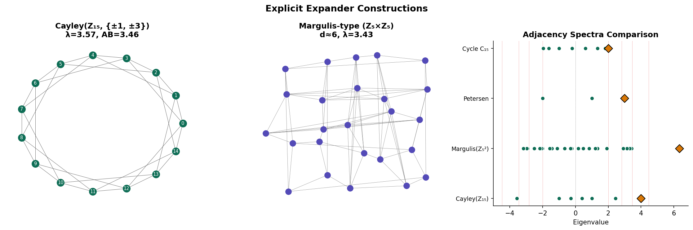
Petersen graph ($n = 10$, $d = 3$). This remarkable 3-regular graph has:

• $h_V = 1$ (every subset of size $\leq 5$ has at least as many external neighbors).
• $h(G) = 2$ (verified by exhaustive search over subsets).
• Adjacency eigenvalues: $3$ (once), $1$ (with multiplicity 5), $-2$ (with multiplicity 4). So $\lambda = 2$.

The Petersen graph is a good expander for its size. We will see shortly that $\lambda = 2$ actually meets the Ramanujan bound $2\sqrt{d-1} = 2\sqrt{2} \approx 2.83$ — it is a Ramanujan graph.

Hypercube $Q_k$ ($n = 2^k$, $d = k$). The $k$-dimensional hypercube has vertices $\{0,1\}^k$ with edges between strings differing in one bit. The adjacency eigenvalues are $k - 2j$ for $j = 0, \ldots, k$, with multiplicity $\binom{k}{j}$. So $\lambda_2 = k - 2$ and $\lambda(Q_k) = k - 2$.

The spectral gap is $d - \lambda = 2$, which is constant — the hypercube is an expander family. Its edge expansion is $h(Q_k) \geq 1$ (the edge-isoperimetric inequality for the cube), and the mixing time of a random walk is $\Theta(k \log k)$.

Barbell graph ($n = 2m$, irregular). Two complete graphs $K_m$ joined by a single edge. The edge connecting them is a severe bottleneck: $h(G) = 1/m \to 0$. The barbell is the canonical non-expander — a single edge cut isolates half the graph.

Graph	$n$	$d$	$h_V(G)$	$h(G)$	$\lambda(G)$	Expander?
$K_n$	$n$	$n-1$	$\geq 1$	$\geq n/2$	$1$	Yes (not sparse)
$C_n$	$n$	$2$	$\to 0$	$\to 0$	$2 - O(1/n^2)$	No
Petersen	$10$	$3$	$1$	$2$	$2$	Yes
$Q_k$	$2^k$	$k$	$\geq 1$	$\geq 1$	$k-2$	Yes (degree grows)
Barbell	$2m$	varies	$\to 0$	$\to 0$	$\to d$	No

Graph:PetersenHypercube Q₃Hypercube Q₄Cycle(n)Path(n)Barbell(k+k)Random 3-regularRandom 4-regularComplete(n)Cayley ℤₙ {±1,±2}

+ Add edge− Remove edge

Expansion Metrics

h_V(G)Vertex expansion

0.800

h(G)Edge expansion

1.000

λ(G)Spectral parameter

2.000

2√(d−1)

Ramanujan: ✓ Yes — \u03BB(G) = 2.000 ≤ 2.828 = 2√(d−1)

d = 3

---

2. The Relationship Between Expansion Notions

Before proving the deep equivalence via Cheeger’s inequality, we establish a direct relationship between vertex and edge expansion.

This tells us that vertex and edge expansion differ by at most a factor of $d$. For constant-degree graphs (the setting we care about for expander families), the two notions are equivalent up to a constant.

---

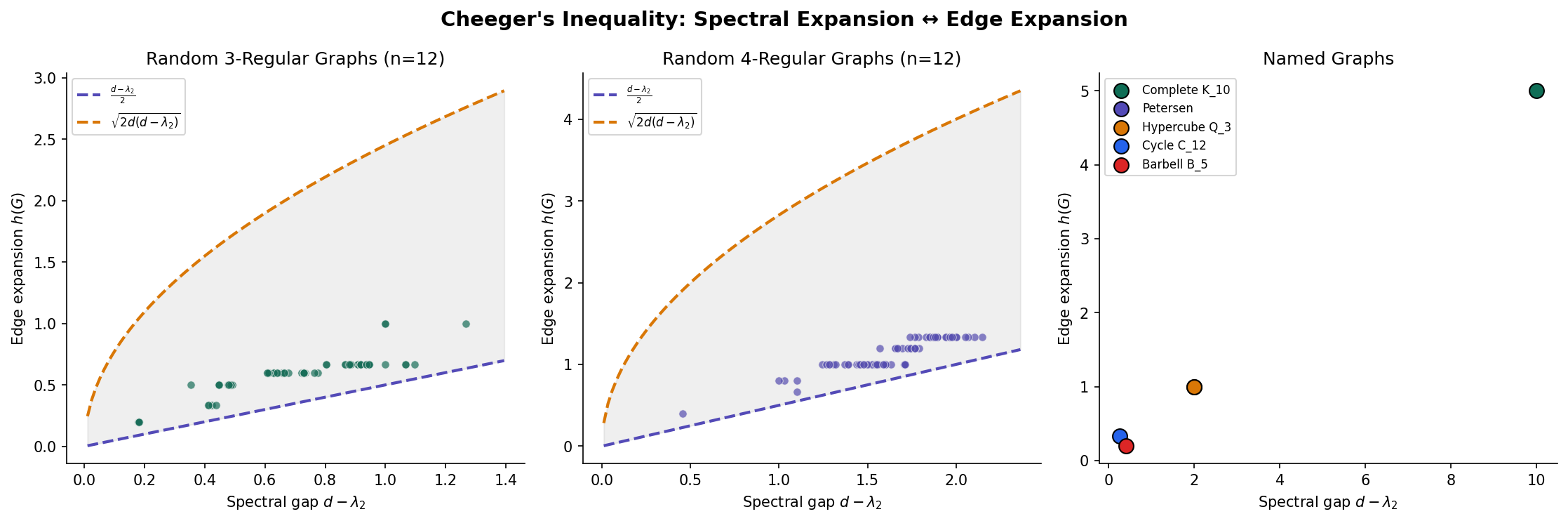
3. Cheeger’s Inequality: Linking Spectrum to Combinatorics

The crown jewel of spectral graph theory is Cheeger’s inequality, which asserts that the spectral gap and the Cheeger constant determine each other up to polynomial factors. We proved a version of this in Graph Laplacians & Spectrum; here we state and prove the version tailored to the adjacency matrix of regular graphs.

This equivalence is why we can speak of “expander families” without specifying which notion of expansion — for constant-degree regular graphs, all three notions agree up to polynomial transformations of the expansion parameter.

---

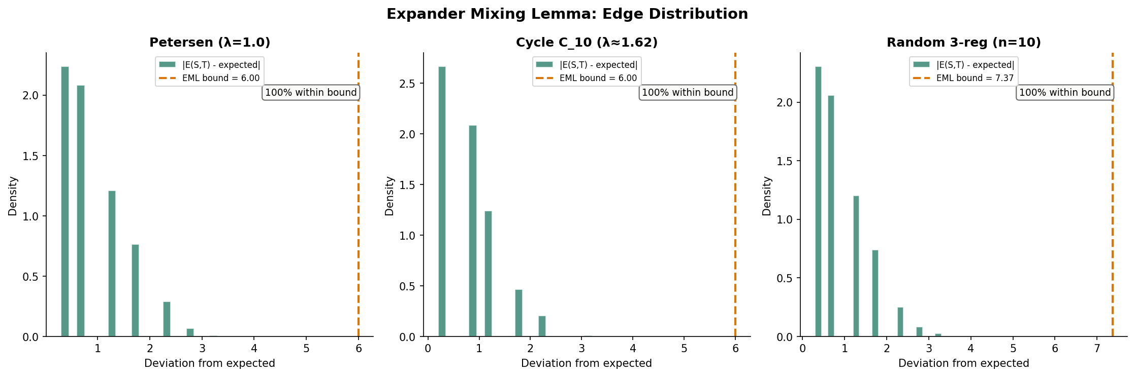
4. The Expander Mixing Lemma

The Expander Mixing Lemma (EML) is the most quantitatively useful consequence of spectral expansion. While the Cheeger constant controls cuts for the worst-case set $S$, the EML controls the number of edges between any two sets $S$ and $T$, making it a powerful tool for combinatorial arguments.

In a random $d$-regular graph (or equivalently, in a $d$-regular graph chosen uniformly from all edge configurations), the expected number of edges between two disjoint sets $S$ and $T$ is $d|S||T|/n$ — each of the $d|S|$ edge-endpoints in $S$ hits $T$ with probability roughly $|T|/n$. The EML says that in an $(n, d, \lambda)$-expander, the actual count deviates from this expected value by at most $\lambda\sqrt{|S||T|}$.

The EML is a multiplicative guarantee when $S$ and $T$ are not too small. If $|S| = |T| = \alpha n$ for some constant $\alpha$, the expected edge count is $d\alpha^2 n$ and the error bound is $\lambda \alpha n$. The relative error is $\lambda/(d\alpha)$, which is $O(\lambda/d)$ — small when $\lambda \ll d$.

4.1 Consequences of the EML

The EML has immediate combinatorial consequences:

Edge density. Setting $T = S$: the number of edges within $S$ satisfies $|E(S,S) - d|S|^2/n| \leq \lambda|S|$. The term $E(S,S)$ counts twice each edge inside $S$, so the actual edge count is $e(S) = E(S,S)/2$, and:

$\left|e(S) - \frac{d|S|^2}{2n}\right| \leq \frac{\lambda |S|}{2}$

This says internal edge density is close to $d|S|/(2n)$ per vertex — nearly what you would expect from a random graph.

Independence number. An independent set $S$ has $e(S) = 0$, so $d|S|^2/(2n) \leq \lambda|S|/2$, giving:

$|S| \leq \frac{\lambda n}{d}$

For an $(n, d, \lambda)$-expander with $\lambda/d$ small, the independence number is at most a $\lambda/d$ fraction of $n$. This is a non-trivial bound: it says expansion forces edges to spread evenly, making large independent sets impossible.

Chromatic number. Combining the independence number bound with a greedy coloring argument gives $\chi(G) \geq d/\lambda$ — expanders need many colors.

Graph:Petersen graphCycle(10)Random 3-regular(10)Random 4-regular(10)

Click adds to:ST

k:3

Random S, TClear selection

S (0)T (0)S \u2229 Tedges between S and T

---

5. Ramanujan Graphs and the Alon-Boppana Bound

We now ask: how small can $\lambda(G)$ be for a $d$-regular graph? A smaller $\lambda$ means better expansion, tighter EML bounds, and faster mixing. Is there a limit?

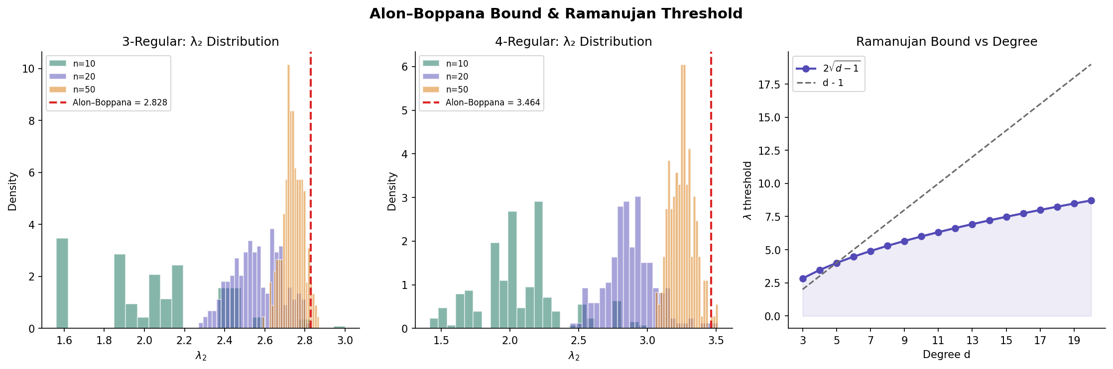
5.1 The Alon-Boppana Lower Bound

The answer is yes: there is a universal floor that no infinite family of $d$-regular graphs can beat.

The Alon-Boppana bound tells us that $2\sqrt{d-1}$ is an impassable barrier: no family of $d$-regular graphs can have $\lambda < 2\sqrt{d-1}$ for all but finitely many members. This leads to the definition of optimal expanders.

5.2 Ramanujan Graphs

Ramanujan graphs are the best possible expanders for their degree: they meet the Alon-Boppana bound with equality. The name honors the Indian mathematician Srinivasa Ramanujan, whose conjectures about modular forms (proved by Deligne) are the key ingredient in the original constructions.

5.3 Examples of Ramanujan Graphs

Petersen graph ($d = 3$, $n = 10$). The eigenvalues are $\{3, 1, 1, 1, 1, 1, -2, -2, -2, -2\}$. We need $\lambda(G) = \max(|1|, |-2|) = 2$. The Ramanujan bound is $2\sqrt{3 - 1} = 2\sqrt{2} \approx 2.83$. Since $2 \leq 2.83$, the Petersen graph is Ramanujan.

Complete graph $K_n$ ($d = n - 1$). The non-trivial eigenvalues are all $-1$, so $\lambda(K_n) = 1$. The Ramanujan bound is $2\sqrt{n-2}$. For $n \geq 3$, we have $1 \leq 2\sqrt{n-2}$, so every $K_n$ is Ramanujan. (This is expected — the complete graph is the best possible expander, but it is not sparse.)

Cycle $C_n$ ($d = 2$). The Ramanujan bound is $2\sqrt{1} = 2$. The second-largest eigenvalue is $\lambda_2 = 2\cos(2\pi/n) < 2$ for $n \geq 3$, so every cycle is technically Ramanujan. This may seem surprising, but recall that the cycle is not a good expander — the Cheeger constant $h(C_n) \to 0$. Ramanujan-ness at $d = 2$ is vacuous because $2\sqrt{d-1} = 2 = d$, so the condition imposes no constraint beyond regularity.

Complete bipartite graph $K_{n/2, n/2}$ ($d = n/2$). The eigenvalues are $n/2$, $0$ (with multiplicity $n-2$), and $-n/2$. Here $\lambda_n = -d$, which means $|\lambda_n| = d$. Under our definition, $\lambda(G) = \max_{i \geq 2}|\lambda_i| = d$, so $\lambda(G) = d$. However, the Ramanujan condition for bipartite graphs uses the nontrivial spectral parameter

$\lambda_{\mathrm{nt}}(G) := \max\{|\lambda_i(A)| : |\lambda_i| < d\}$

which excludes both the trivial eigenvalues $+d$ and $-d$. With this convention, $\lambda_{\mathrm{nt}}(K_{n/2, n/2}) = 0$, and $K_{n/2, n/2}$ is trivially Ramanujan (but again, not sparse). We use $\lambda_{\mathrm{nt}}(G)$ in the table below and in the Ramanujan check of the interactive visualizations.

Graph	$d$	$\lambda_{\mathrm{nt}}(G)$	$2\sqrt{d-1}$	Ramanujan?
Petersen	3	2	2.83	Yes
$K_5$	4	1	3.46	Yes
$K_6$	5	1	4.00	Yes
$C_n$	2	$2\cos(2\pi/n)$	2	Yes (vacuous)
Hypercube $Q_4$	4	2	3.46	Yes
Random 3-regular	3	$\approx 2\sqrt{2}$	2.83	Nearly

Degree d:

3456

n:30Ensemble:50100200

Computing ensemble spectra...

---

6. Explicit Constructions

One of the remarkable features of expander graphs is that they can be constructed explicitly — we do not need randomness to build them. This section describes two families of constructions: algebraic constructions from Cayley graphs and the number-theoretic LPS construction.

6.1 Cayley Graphs

Cayley graphs are a natural source of highly structured regular graphs. Their spectral properties are determined by the representation theory of the group $\Gamma$ — and for abelian groups, the eigenvalues have an explicit formula.

6.2 The Margulis-Gabber-Galil Construction

The first explicit expander family was constructed by Margulis (1973), with the spectral gap proved by Gabber and Galil (1981). It produces 8-regular graphs on $n^2$ vertices.

Construction. Let $n$ be any positive integer. Define the graph $G_n$ on the vertex set $\mathbb{Z}_n \times \mathbb{Z}_n$ (so $|V| = n^2$) with edges from $(x, y)$ to each of:

$(x \pm 1, y), \quad (x, y \pm 1), \quad (x + y, y), \quad (x - y, y), \quad (x, y + x), \quad (x, y - x)$

where all arithmetic is modulo $n$. Some of these eight neighbors may coincide, but in general the graph is 8-regular.

Why is this an expander? The generating set $S$ includes both “translation” moves (adding $\pm 1$ to a coordinate) and “shear” moves (adding one coordinate to the other). The translations provide local connectivity, while the shears — which act as hyperbolic rotations on $\mathbb{Z}_n^2$ — spread out any concentrated set of vertices rapidly. The spectral gap satisfies $\lambda(G_n) \leq 5\sqrt{2} \approx 7.07$, so the spectral gap $8 - \lambda \geq 8 - 5\sqrt{2} \approx 0.93$ is bounded away from zero.

6.3 The LPS Construction

The Lubotzky-Phillips-Sarnak (LPS) construction produces $(p+1)$-regular Ramanujan graphs for primes $p$. The construction uses deep number theory — specifically, Jacobi’s four-square theorem and Ramanujan’s conjecture on modular forms (proved by Deligne).

Sketch of the construction. Fix two distinct odd primes $p$ and $q$ with $p, q \equiv 1 \pmod{4}$. The LPS graph $X^{p,q}$ is the Cayley graph of $\mathrm{PGL}(2, \mathbb{F}_q)$ — the projective general linear group of $2 \times 2$ invertible matrices over the finite field $\mathbb{F}_q$ — with generating set determined by the $(p+1)$ representations of $p$ as a sum of four squares:

$p = a_0^2 + a_1^2 + a_2^2 + a_3^2$

where $a_0 > 0$ is odd and $a_1, a_2, a_3$ are even. Each representation yields a matrix in $\mathrm{PGL}(2, \mathbb{F}_q)$, and these matrices form a symmetric generating set of size $p+1$.

The Ramanujan property $\lambda(X^{p,q}) \leq 2\sqrt{p}$ follows from deep results: the non-trivial eigenvalues of the Cayley graph are expressed in terms of Hecke eigenvalues of automorphic forms on $\mathrm{GL}(2)$, and Ramanujan’s conjecture (now Deligne’s theorem) bounds these eigenvalues.

6.4 Constructing Cayley Graphs in Practice

Here is a Python implementation of Cayley graph construction for cyclic groups:

import numpy as np
from itertools import product

def cayley_graph_cyclic(n, generators):
    """
    Build the adjacency matrix of Cay(Z_n, S)
    where S = generators ∪ {-g mod n : g in generators}.
    """
    # Symmetrize the generating set
    S = set()
    for g in generators:
        S.add(g % n)
        S.add((-g) % n)
    S.discard(0)  # Remove identity

    A = np.zeros((n, n), dtype=int)
    for v in range(n):
        for s in S:
            w = (v + s) % n
            A[v, w] = 1
    return A, sorted(S)

def margulis_gabber_galil(n):
    """
    Build the Margulis–Gabber–Galil 8-regular expander on Z_n × Z_n.
    Returns adjacency matrix of size n^2 × n^2.
    """
    N = n * n
    A = np.zeros((N, N), dtype=int)

    def idx(x, y):
        return (x % n) * n + (y % n)

    for x in range(n):
        for y in range(n):
            i = idx(x, y)
            neighbors = [
                idx(x + 1, y), idx(x - 1, y),
                idx(x, y + 1), idx(x, y - 1),
                idx(x + y, y), idx(x - y, y),
                idx(x, y + x), idx(x, y - x),
            ]
            for j in neighbors:
                A[i, j] = 1
    return A

---

7. Random Walks on Expanders

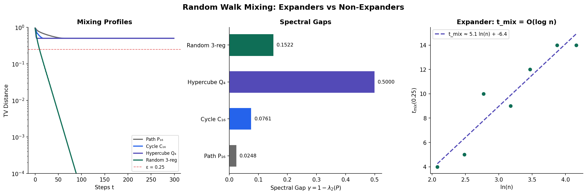
In Random Walks & Mixing, we proved that the mixing time of a random walk is controlled by the spectral gap: $t_{\mathrm{mix}} = O(1/\gamma \cdot \log n)$ where $\gamma = 1 - \lambda_2(P)$. For expanders, $\gamma$ is bounded away from zero, so the mixing time is $O(\log n)$ — logarithmic in the number of vertices.

7.1 Mixing Time on Expanders

7.2 Comparison of Mixing Times

The following table compares mixing times across graph families, highlighting how expansion controls convergence speed:

Graph Family	$n$	$d$	$\lambda(G)$	Spectral Gap $d - \lambda$	$t_{\mathrm{mix}}$
Path $P_n$	$n$	2	$2\cos(\pi/n)$	$O(1/n^2)$	$\Theta(n^2)$
Cycle $C_n$	$n$	2	$2\cos(2\pi/n)$	$O(1/n^2)$	$\Theta(n^2)$
Hypercube $Q_k$	$2^k$	$k$	$k-2$	$2$	$\Theta(k \log k)$
$(n, d, \lambda)$-Expander	$n$	$d$	$\lambda$	$d - \lambda = \Theta(1)$	$\Theta(\log n)$
Complete $K_n$	$n$	$n-1$	1	$n-2$	$\Theta(1)$

The path and cycle have vanishing spectral gap, so mixing takes polynomial time. The hypercube has a constant spectral gap (2) and mixes in $O(n \log n)$ where $n = \log_2 |V|$. Expanders achieve the optimal $O(\log |V|)$ mixing for sparse graphs.

---

8. Applications to Computer Science and Machine Learning

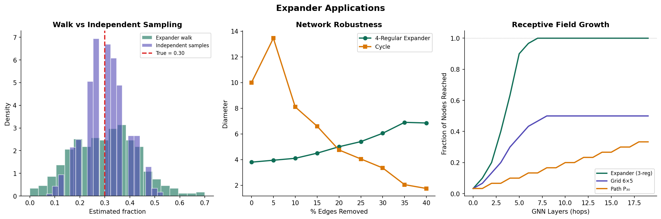
8.1 Expander Walk Sampling and Derandomization

The most celebrated application of expanders in theoretical computer science is derandomization: reducing the amount of randomness needed by a probabilistic algorithm. The key result is the expander walk sampling theorem.

This is a Chernoff-type concentration bound for dependent samples. In a standard Chernoff bound for $t$ independent samples, the exponent is $-\varepsilon^2 t / 2$. The expander walk version has an extra factor of $1 - \lambda/d$ (the spectral gap of the walk) — a mild penalty for dependence.

Why is this useful for derandomization? To sample $t$ independent vertices from $G$, you need $t \log n$ random bits. But a random walk of length $t$ on $G$ requires only $\log n$ bits (for the starting vertex) plus $t \log d$ bits (for the $t$ neighbor choices), totaling $\log n + t \log d$. When $d$ is a constant and $t = O(\log n)$, this is $O(\log n)$ — exponentially fewer random bits than independent sampling. The expander walk sampling theorem guarantees that the walk’s samples are “almost as good” as independent samples.

This principle underlies the Ajtai-Komlós-Szemerédi (AKS) sorting network, the Impagliazzo-Zuckerman extractor, and many other constructions in derandomization and pseudorandomness.

8.2 Error-Correcting Codes

Sipser and Spielman (1996) showed that bipartite expander graphs yield error-correcting codes with remarkable properties:

Construction. Start with a bipartite $(c, d)$-regular expander $G = (L \cup R, E)$ where $|L| = n$, $|R| = m$. Each right vertex $r \in R$ imposes a parity check: the bits indexed by $N(r) \subseteq L$ must sum to 0 modulo 2. The resulting code has:

• Block length $n$
• Rate $1 - m/n$ (approaches $1 - c/d$ for good expanders)
• Minimum distance proportional to $n$ (linear distance, from the expansion property)
• Linear-time decoding: the expansion guarantees a simple “flip” algorithm converges in $O(n)$ steps

The expansion property is the key: if a codeword has $\delta n$ errors for small enough $\delta$, the $\delta n$ erroneous bits have at least $(1 - \varepsilon)c \cdot \delta n$ unsatisfied check nodes (by vertex expansion), which is more than the $\varepsilon c \cdot \delta n$ checks that could be satisfied by accident. The decoder identifies and corrects errors by examining local check violations.

8.3 Network Robustness

Expander graphs are optimally robust networks: removing a constant fraction of vertices or edges still leaves a connected graph (in fact, a graph that is itself an expander). Formally:

• Vertex robustness: Removing any $\alpha n$ vertices from an $(n, d, \lambda)$-expander leaves a connected graph, provided $\alpha$ is smaller than a threshold depending on $d$ and $\lambda$.
• Edge robustness: Similarly, removing edges. The Cheeger constant lower bound guarantees that every cut has at least $h(G) \cdot |S| \geq (d - \lambda)/2 \cdot |S|$ edges, so creating a disconnection requires removing $\Omega(n)$ edges.

These properties make expanders ideal for communication networks, peer-to-peer systems, and distributed hash tables, where robustness to node failures is essential.

8.4 Graph Neural Networks and Over-Smoothing

---

9. Computational Notes

9.1 Computing Expansion Metrics

Here is a complete implementation for computing spectral expansion metrics and checking the Ramanujan property:

import numpy as np
from scipy import linalg

def expansion_metrics(A):
    """
    Compute spectral expansion metrics for a d-regular graph
    with adjacency matrix A.

    Returns a dictionary with degree, lambda (spectral expansion parameter),
    spectral gap, Ramanujan bound, and whether the graph is Ramanujan.
    """
    eigenvalues = np.sort(linalg.eigvalsh(A))[::-1]
    d = eigenvalues[0]

    # lambda = max |lambda_i| for i >= 2
    # For non-bipartite graphs, also exclude lambda_n = -d
    nontrivial = eigenvalues[1:]
    if np.isclose(nontrivial[-1], -d, atol=1e-8):
        # Bipartite: exclude -d as trivial
        nontrivial = nontrivial[:-1]

    lambda_val = np.max(np.abs(nontrivial))
    ram_bound = 2 * np.sqrt(d - 1)

    return {
        'degree': d,
        'lambda': lambda_val,
        'spectral_gap': d - eigenvalues[1],
        'ramanujan_bound': ram_bound,
        'is_ramanujan': lambda_val <= ram_bound + 1e-10,
        'eigenvalues': eigenvalues
    }

9.2 Verifying the Expander Mixing Lemma

def verify_eml(A, S_indices, T_indices):
    """
    Verify the Expander Mixing Lemma for subsets S and T.

    Returns the actual edge count E(S,T), the expected count d|S||T|/n,
    the EML bound lambda * sqrt(|S||T|), and whether the bound holds.
    """
    n = A.shape[0]
    metrics = expansion_metrics(A)
    d = metrics['degree']
    lam = metrics['lambda']

    # Count edges from S to T (ordered pairs)
    E_ST = sum(A[i, j] for i in S_indices for j in T_indices)

    expected = d * len(S_indices) * len(T_indices) / n
    bound = lam * np.sqrt(len(S_indices) * len(T_indices))
    deviation = abs(E_ST - expected)

    return {
        'E_ST': E_ST,
        'expected': expected,
        'deviation': deviation,
        'eml_bound': bound,
        'bound_holds': deviation <= bound + 1e-10
    }

# Example: Petersen graph
def petersen_adjacency():
    """Return the 10x10 adjacency matrix of the Petersen graph."""
    edges = [
        (0,1),(0,4),(0,5), (1,2),(1,6), (2,3),(2,7),
        (3,4),(3,8), (4,9), (5,7),(5,8), (6,8),(6,9), (7,9)
    ]
    A = np.zeros((10, 10), dtype=int)
    for i, j in edges:
        A[i, j] = A[j, i] = 1
    return A

A = petersen_adjacency()
metrics = expansion_metrics(A)
print(f"Petersen: d={metrics['degree']:.0f}, "
      f"λ={metrics['lambda']:.4f}, "
      f"Ramanujan bound={metrics['ramanujan_bound']:.4f}, "
      f"Ramanujan={metrics['is_ramanujan']}")
# Output: Petersen: d=3, λ=2.0000, Ramanujan bound=2.8284, Ramanujan=True

# Verify EML for S = {0,1,2}, T = {5,6,7,8,9}
result = verify_eml(A, [0,1,2], [5,6,7,8,9])
print(f"E(S,T)={result['E_ST']}, expected={result['expected']:.2f}, "
      f"deviation={result['deviation']:.2f}, bound={result['eml_bound']:.2f}, "
      f"holds={result['bound_holds']}")

9.3 Building and Analyzing Margulis-Gabber-Galil Expanders

def analyze_mgg_family(n_values):
    """
    Analyze the Margulis–Gabber–Galil expander family
    for several values of n, verifying the spectral gap
    stays bounded away from zero.
    """
    results = []
    for n in n_values:
        A = margulis_gabber_galil(n)
        metrics = expansion_metrics(A)
        results.append({
            'n': n,
            'vertices': n * n,
            'degree': metrics['degree'],
            'lambda': metrics['lambda'],
            'spectral_gap': metrics['spectral_gap'],
            'is_ramanujan': metrics['is_ramanujan']
        })
        print(f"MGG(n={n}): {n*n} vertices, d={metrics['degree']:.0f}, "
              f"λ={metrics['lambda']:.2f}, gap={metrics['spectral_gap']:.2f}")
    return results

# Example output (approximate):
# MGG(n=5): 25 vertices, d=8, λ=6.47, gap=1.53
# MGG(n=7): 49 vertices, d=8, λ=6.83, gap=1.17
# MGG(n=11): 121 vertices, d=8, λ=7.02, gap=0.98

For the full interactive analysis with additional graph families and larger experiments, see the companion notebook.

---

10. Connections and Further Reading

10.1 Connections to Other Topics

Topic	Connection
Graph Laplacians & Spectrum	Cheeger’s inequality links the Laplacian spectral gap to edge expansion. The Fiedler vector provides a spectral approximation to the minimum cut, and expanders are precisely the graphs where this cut is large for every subset.
Random Walks & Mixing	The mixing time of a random walk on an expander is $O(\log n)$, because the spectral gap $\gamma = 1 - \lambda/d$ is bounded away from zero. The expander walk sampling theorem extends this to a Chernoff bound for dependent samples.
Spectral Theorem	The EML proof decomposes indicator vectors in the eigenbasis of $A$. The Spectral Theorem guarantees orthonormality of this basis — the Cauchy-Schwarz step relies on this structure.
Concentration Inequalities	The expander walk sampling theorem is a Chernoff bound where the spectral gap replaces independence. Correlations between consecutive walk samples decay exponentially in the gap.
Shannon Entropy	The entropy rate of a random walk on a $d$-regular expander approaches $\log d$ — maximum entropy. Expansion ensures the walk explores the graph uniformly.
Message Passing & GNNs	Message passing is iterated Laplacian smoothing. On expanders, $O(\log n)$ layers suffice for global information flow but cause over-smoothing. The spectral gap quantifies this trade-off.

10.2 Notation Summary

Symbol	Meaning
$G = (V, E)$	Graph with vertex set $V$ and edge set $E$
$n = \vert V\vert$	Number of vertices
$d$	Degree (for regular graphs)
$A$	Adjacency matrix
$\lambda_i(A)$	$i$-th eigenvalue of $A$ (ordered $\lambda_1 \geq \cdots \geq \lambda_n$)
$\lambda(G)$	Spectral expansion parameter: $\max_{i \geq 2} \vert\lambda_i(A)\vert$
$h(G)$	Cheeger constant (edge expansion)
$h_V(G)$	Vertex expansion ratio
$P = D^{-1}A$	Random walk transition matrix
$\gamma = 1 - \lambda/d$	Spectral gap of the random walk
$t_{\mathrm{mix}}$	Mixing time in total variation
$E(S, T)$	Number of (ordered) edges from $S$ to $T$
$\partial_V(S)$	Vertex boundary: $N(S) \setminus S$
$2\sqrt{d-1}$	Alon-Boppana / Ramanujan bound