The Information Bottleneck

1. What problem does the information bottleneck solve?

1.1 Predictive but compact: the trade-off as a design principle

Representations sit between raw data and downstream tasks. A useful representation does two opposed things at once: it throws away what the task doesn’t need (so we aren’t swamped by noise), and it keeps what the task does need (so we can still answer the question). The information bottleneck principle formalizes exactly that opposition as a single optimization problem.

The setup names three random variables. The input $X$ is whatever the world hands us — a document, an image, a sensor trace. The target $Y$ is whatever we ultimately care about — a topic label, a class, a downstream measurement. The representation $T$ is the compressed object we want to learn, and we require $T$ to be a (possibly stochastic) function of $X$ alone. Formally, $T$ is conditionally independent of $Y$ given $X$:

$Y \;\to\; X \;\to\; T,$

which is the Markov chain we’ll be working inside for the rest of the topic. Concretely, $T$‘s distribution is fully specified by an encoder $p(t \mid x)$ — the only knob the IB principle gets to turn.

Two strategies fail immediately. If we set $T = X$, the encoder is the identity; we have compressed nothing and we have learned nothing. If we set $T$ to a constant, the encoder throws everything away; we have compressed perfectly and we have predicted nothing. Useful representations live in between, and the IB principle picks the trade-off explicitly via the Lagrangian

$\mathcal{L}_\beta\bigl(p(t\mid x)\bigr) \;=\; I(X;T) \;-\; \beta\, I(T;Y), \qquad \beta > 0. \quad\quad (1.1)$

The first term is the cost of remembering: how much information about $X$ leaks through the encoder. The second is the value of predicting: how much information about $Y$ the representation $T$ retains. The single scalar $\beta$ shifts where we want to land between the two failure modes. As $\beta \to 0$, only compression matters and the minimizer collapses to a constant. As $\beta \to \infty$, only prediction matters and the minimizer recovers the lossless representation. Everything interesting happens in between, on the IB curve — the Pareto frontier in the $(I(X;T),\, I(T;Y))$ plane traced out as $\beta$ sweeps.

We will rederive every piece of this picture over the next eleven sections. For now, it is enough to know that we have a single-parameter family of optimization problems and that the parameter has an interpretable meaning: $\beta$ is the bit-for-bit exchange rate between compression and prediction.

1.2 A motivating vignette: clustering documents by topic

The original Tishby–Pereira–Bialek paper grounds the principle in document clustering, which is still the cleanest first example. Imagine eight documents drawn from two hidden topics — call them “sports” and “finance.” Each document $x \in \{0,1,\ldots,7\}$ is summarized by a word-count signature, and the topic label $y \in \{0,1\}$ is what a downstream task cares about. A representation $T$ is a (soft) clustering: the encoder $p(t \mid x)$ says how strongly document $x$ is assigned to cluster $t$.

We give every document equal mass and arrange the topic structure as cleanly as possible: documents $0$ through $3$ come from topic $0$, documents $4$ through $7$ from topic $1$. The joint distribution $p(x,y)$ then has uniform mass $1/8$ on its eight-point support, and the marginals come out to $p(x) = 1/8$ for every document and $p(y) = 1/2$ for each topic. Quick consequences:

$H(X) = \log_2 8 = 3, \qquad H(Y) = \log_2 2 = 1, \qquad I(X;Y) = H(Y) = 1.$

The last equality uses that $Y$ is a deterministic function of $X$ on this construction, so $H(Y\mid X) = 0$ and $I(X;Y) = H(Y) - H(Y\mid X) = 1$.

Three reference clusterings stake out the corners of the IB plane:

Clustering	$I(X;T)$	$I(T;Y)$	What it does
$T = \text{const}$	$0$	$0$	Full compression. All documents in one cluster — predictiveness destroyed.
$T = Y$	$1$	$1$	Topic-aligned. Two clusters, one per topic — minimum compression that still captures all of $Y$.
$T = X$	$3$	$1$	Identity. Eight clusters, one per document — zero compression, but no additional predictiveness over $T = Y$.

The third row is the punchline: keeping all three bits of $X$ buys exactly the same one bit of $Y$-information as keeping only the one bit that says “which topic.” Compressing $X$ from three bits down to one bit is therefore free on this construction — the extra two bits of $X$ are pure noise from $Y$‘s point of view. The IB curve, traced over $\beta$, will recover this fact algorithmically without being told what $Y$ is in advance. We come back to this same eight-document table in §5 when we run the discrete IB algorithm on it.

Reference clusteringT = const (full compression)T = topic (T = Y)4 clusters, topic-pure pairsT = X (identity)Mis-aligned 2-cluster split

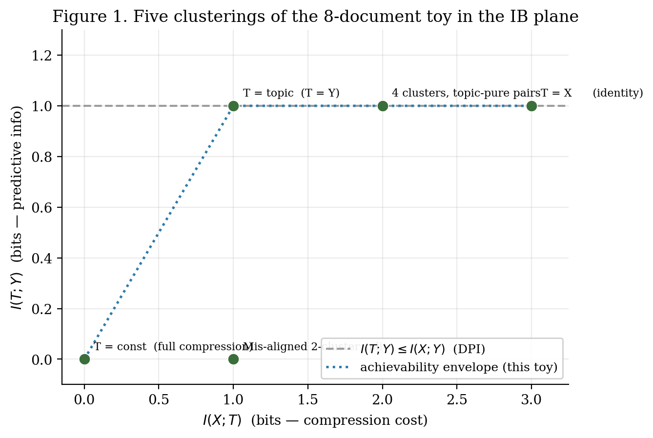
Two clusters aligned with the two topics. Captures all of Y at the smallest possible I(X;T) — sits on the optimal corner of the IB plane.

Assignment p(t | x)

I(X;T) = 1.000 bits

I(T;Y) = 1.000 bits

1.3 Why mutual information is the right currency

Why measure “informativeness” with mutual information rather than (say) classification accuracy, correlation, or one of the many divergences floating around in the ML literature? Four reasons make MI the natural choice for both axes of the IB plane.

Invariance to relabeling. $I(X;T)$ depends only on the joint distribution $p(x,t)$, not on how cluster names are assigned. Two clusterings that partition $X$ identically have the same mutual information regardless of whether we call the clusters "$\{0,1\}$" or ”$\{\text{sports}, \text{finance}\}$.” Compression should count statistical structure, not labels, and MI does this by construction.

A coding interpretation. Shannon’s source-coding theorem (the foundation we lean on from Shannon entropy) tells us that $I(X;T)$ is, asymptotically, the average number of bits per sample needed to communicate $T$ to a receiver who already knows $X$. So $I(X;T)$ has a literal units interpretation — bits. The compression term in the IB Lagrangian carries a cost in the same currency as the predictiveness term.

A clean entropy decomposition. Writing $H(X) = I(X;T) + H(X \mid T)$ splits the entropy of $X$ into “the bits about $X$ captured by $T$” and “the bits about $X$ lost in $T$.” Maximizing $I(X;T)$ is exactly minimizing what we lose; minimizing $I(X;T)$ is exactly maximizing what we throw away. The IB Lagrangian is asking us to throw away what is irrelevant and to keep what is relevant, both measured in the same units.

The data-processing inequality. For any Markov chain $T \leftarrow X \to Y$,

$I(T;Y) \;\le\; I(X;Y). \quad\quad (1.2)$

No matter what encoder we cook up from $X$, the representation $T$ cannot predict $Y$ better than $X$ itself can. This places a hard ceiling on the predictiveness side of the IB plane: the IB curve is bounded above by the constant $I(X;Y)$. It also tells us when compression is genuinely free. If $I(X;Y) \ll H(X)$ — that is, if $X$ has lots of bits unrelated to $Y$ — then there is plenty of room to compress without paying anything in predictiveness. Our document-clustering toy has $H(X) = 3$ and $I(X;Y) = 1$, so two of the three bits in $X$ are pure noise from $Y$‘s standpoint, and the IB algorithm will discard them as $\beta$ varies.

These four properties together — invariance, units, decomposition, the DPI ceiling — make $I(X;T)$ and $I(T;Y)$ the natural axes of the trade-off. The IB Lagrangian is, in a real sense, the most parsimonious functional you can write that respects all four.

1.4 Roadmap and what’s not in scope

The topic covers three substantive arcs.

Discrete IB (Tishby–Pereira–Bialek 1999), §§3–5. We derive the stationarity conditions on $\mathcal{L}_\beta$ by variational calculus on the encoder, obtain the three coupled updates for $p(t\mid x)$, $p(t)$, and $p(y\mid t)$, prove convergence of the iterative algorithm via a Lyapunov argument inherited from the Blahut–Arimoto algorithm in rate-distortion theory, and run the algorithm on the eight-document toy to trace out the IB curve.

Gaussian IB (Chechik–Globerson–Tishby–Weiss 2005), §§6–7. When $(X,Y)$ are jointly Gaussian, the IB problem has a closed-form solution: the optimal encoder is linear-plus-Gaussian-noise, and the optimal projection directions are the canonical-correlation directions of $\Sigma_X^{-1/2}\, \Sigma_{X\mid Y}\, \Sigma_X^{-1/2}$. The IB curve becomes piecewise-analytic, with phase transitions at critical $\beta_c$ values where new directions activate. This is the analytical sandbox where every quantity is exactly computable.

Variational IB and the deep-learning lift, §§8–10. The Alemi–Fischer–Dillon–Murphy 2017 variational lower bound on $-\mathcal{L}_\beta$ makes the IB Lagrangian tractable for encoders that are too high-dimensional to enumerate, including neural-network encoders. We will derive the bound, work through the reparametrization trick, and exercise the construction on a closed-form linear-Gaussian VIB sandbox. Then we take the deep-learning controversy head-on: Tishby–Zaslavsky 2015 and Shwartz-Ziv–Tishby 2017 argued that deep networks generically traverse a “fitting then compression” trajectory in the information plane; Saxe et al. 2018 showed that the compression phase disappears when the activation is ReLU instead of tanh, and may have been an artifact of how MI was estimated. We will present both sides faithfully.

Connections and limits, §§11–12. IB is mathematically adjacent to several other principles: rate-distortion (the closest parent — same Lagrangian template, different distortion), PAC-Bayes (which uses a KL term as a complexity penalty, structurally analogous to the $I(X;T)$ term), and InfoNCE in contrastive learning (which is provably an MI lower bound, so contrastive methods are implicitly doing IB-style optimization). We close with computational notes — logsumexp stability, plug-in MI estimator pitfalls — and a list of honest limits.

What we are not doing. We are not training a deep VIB on real image data; the under-60-second CPU runtime budget rules it out, and Alemi et al.’s MNIST numbers will be discussed but not reproduced. We are not adjudicating the deep-learning debate; we will present the controversy faithfully and let the reader form their own view. We are not building a full rate-distortion theory from scratch; that lives in rate-distortion, and we’ll cite forward to it at the relevant point in §11.

2. The information bottleneck Lagrangian

2.1 The setting and the Markov chain

Let $X$ be the input random variable, $Y$ the target, and $T$ the learned representation. We assume the joint distribution $p(x, y)$ is given. In §3 the iterative algorithm will use this distribution directly; in §12.2 we’ll discuss how to estimate it from a finite sample. The triple $(X, Y, T)$ satisfies the Markov property

$Y \;\to\; X \;\to\; T,$

equivalent to the conditional-independence statement $T \perp Y \mid X$. In words: $T$ is allowed to depend on $X$ only through $X$ itself, never directly through $Y$. This is exactly what it means for $T$ to be a (possibly randomized) function of $X$.

The single degree of freedom in the problem is the encoder

$p(t \mid x), \qquad t \in \mathcal{T}.$

We are free to choose the alphabet $\mathcal{T}$, including its cardinality. For the discrete IB of §§3–5 we take $|\mathcal{T}| = k$ for some user-specified $k$; for the Gaussian IB of §§6–7 we take $\mathcal{T} = \mathbb{R}^d$; for the variational IB of §§8–10 the alphabet is whatever the variational family supports.

Three derived distributions matter, and the IB algorithm of §3 will turn out to update exactly these three:

$p(t) \;=\; \sum_x p(x)\,p(t \mid x), \qquad p(x \mid t) \;=\; \frac{p(x)\,p(t \mid x)}{p(t)}, \qquad p(y \mid t) \;=\; \sum_x p(y \mid x)\,p(x \mid t). \quad\quad (2.1)$

The first is the cluster marginal. The second is the cluster-conditional distribution of $X$, by Bayes. The third is the cluster-conditional distribution of $Y$, computed using the Markov property $p(y \mid x, t) = p(y \mid x)$ — the encoder’s job is to forward whatever it knows about $X$, not to invent anything new about $Y$.

2.2 The variational problem

The IB problem has two equivalent forms, and it pays to be precise about both.

The constrained form. Fix a target predictiveness level $I_Y^* \in [0, I(X;Y)]$. The problem is

$\min_{p(t \mid x)} \; I(X; T) \quad \text{subject to} \quad I(T; Y) \ge I_Y^*, \quad \sum_t p(t \mid x) = 1 \; \forall x. \quad\quad (2.2)$

We want the most compressed representation whose predictiveness is at least $I_Y^*$. Sweeping $I_Y^*$ across its allowed range traces out the IB curve.

The Lagrangian form. Introduce a Lagrange multiplier $\beta \ge 0$ for the predictiveness constraint and, for now, handle the normalization constraints implicitly. The Lagrangian we will use from §3 onward is

$\mathcal{F}_\beta(p(t \mid x)) \;=\; I(X; T) \;-\; \beta\, I(T; Y), \qquad \text{minimized over normalized encoders.} \quad\quad (2.3)$

The Lagrangian form is a relaxation: for each $\beta$, the minimizer of $\mathcal{F}_\beta$ also solves (2.2) for some value of $I_Y^*$ (namely the value $I(T;Y)$ achieved by the minimizer), and the two forms generate the same Pareto frontier. We work with the Lagrangian form because its stationarity conditions differentiate cleanly — see §3.2.

A subtlety worth flagging now: the Lagrangian relaxation can miss points on the IB curve where the curve has a corner (i.e., where the right-hand and left-hand slopes disagree). At such points, no single $\beta$ produces that operating point as a Lagrangian minimum — only an open interval of $\beta$ values does, and the achievable point sits “between” the two corner branches. This will matter in §7 when we discuss Gaussian-IB phase transitions, where the curve has exactly such corners.

2.3 The IB curve in the information plane

Define the IB curve as the value function of (2.2):

$I_Y^*(R) \;:=\; \sup_{p(t \mid x)} \Bigl\{\, I(T; Y) \;:\; I(X; T) \le R \,\Bigr\}, \qquad R \in [0, \infty). \quad\quad (2.4)$

This is the upper Pareto boundary of the achievable region in the $(I(X;T), I(T;Y))$ plane — every operating point sits on or below it.

The IB curve is therefore a concave non-decreasing curve starting at the origin, climbing as $R$ grows, and saturating at $I(X; Y)$ once we can afford to encode a sufficient statistic. Past saturation, additional compression budget is wasted on bits of $X$ that don’t help with $Y$. The whole geometric content of the IB principle lives in the shape of this curve.

2.4 What β controls

The Lagrange multiplier $\beta$ in $\mathcal{F}_\beta$ admits a clean geometric reading: it is the reciprocal of the tangent slope of the IB curve at the operating point.

Suppose $p^*(t \mid x)$ minimizes $\mathcal{F}_\beta$ and achieves the point $(R^*, I_Y^*)$ on the IB curve, with $I_Y^* = I_Y^*(R^*)$. By the KKT conditions for problem (2.2), $\beta$ is the dual variable for the predictiveness constraint, and where the curve is differentiable the tangent at $(R^*, I_Y^*)$ has slope $1/\beta$:

$\left.\frac{d I_Y^*}{d R}\right|_{R = R^*} \;=\; \frac{1}{\beta}. \quad\quad (2.5)$

This identity organizes the $\beta$ knob into three regimes.

Small β (large slope, near origin). The compression term dominates the Lagrangian. In the limit $\beta \to 0^+$, the optimum collapses to $R^* = 0$ and $T = \text{const}$.

Large β (small slope, near saturation). The predictiveness term dominates. As $\beta \to \infty$, the optimum recovers a minimal sufficient statistic: $I_Y^* = I(X; Y)$ at the smallest $R$ that supports it.

The critical β_c. Between these regimes sits a sharp threshold. Let $\sigma_0 := \lim_{R \to 0^+} dI_Y^*/dR$ be the initial slope of the IB curve at the origin. For $\beta < 1/\sigma_0$, every nontrivial encoder achieves $\mathcal{F}_\beta > 0$, so the optimum is the trivial $T = \text{const}$. At $\beta_c := 1/\sigma_0$, a nontrivial branch of solutions emerges. For the discrete IB, $\beta_c$ depends on $p(x, y)$ and is generally found numerically by sweeping $\beta$. For the Gaussian IB, $\sigma_0$ equals the largest eigenvalue $\lambda_1$ of a canonical-correlation matrix, so $\beta_c = 1/\lambda_1$ — this is the first of several phase transitions worked out in §7.

A concrete preview makes the picture tangible. The scalar-Gaussian case ($X, Y \in \mathbb{R}$ jointly Gaussian with correlation $\rho$) admits the closed-form IB curve

$I_Y^*(R) \;=\; -\tfrac{1}{2}\log_2\bigl(1 - \rho^2\,(1 - 2^{-2R})\bigr),$

saturating at the predictiveness ceiling $I(X;Y) = -\tfrac{1}{2}\log_2(1 - \rho^2)$. The threshold value $\beta_c = 1/\rho^2$ is the value below which the trivial encoder is optimal. At $\rho = 0.8$, $\beta_c = 1.5625$, and the three tangent operating points referenced by the figure below land at $(0.254, 0.152)$ bits for $\beta = 1.8$, $(1.208, 0.529)$ bits for $\beta = 4$, and $(2.145, 0.674)$ bits for $\beta = 12$ — each with tangent slope $1/\beta$, confirming the KKT identity (2.5). We derive this scalar-Gaussian result formally in §6 and §7; the figure previews the general shape.

Correlation ρ = 0.80 (β_c = 1/ρ² = 1.562)

β = 4.00 (slope at operating point = 1/β = 0.250)

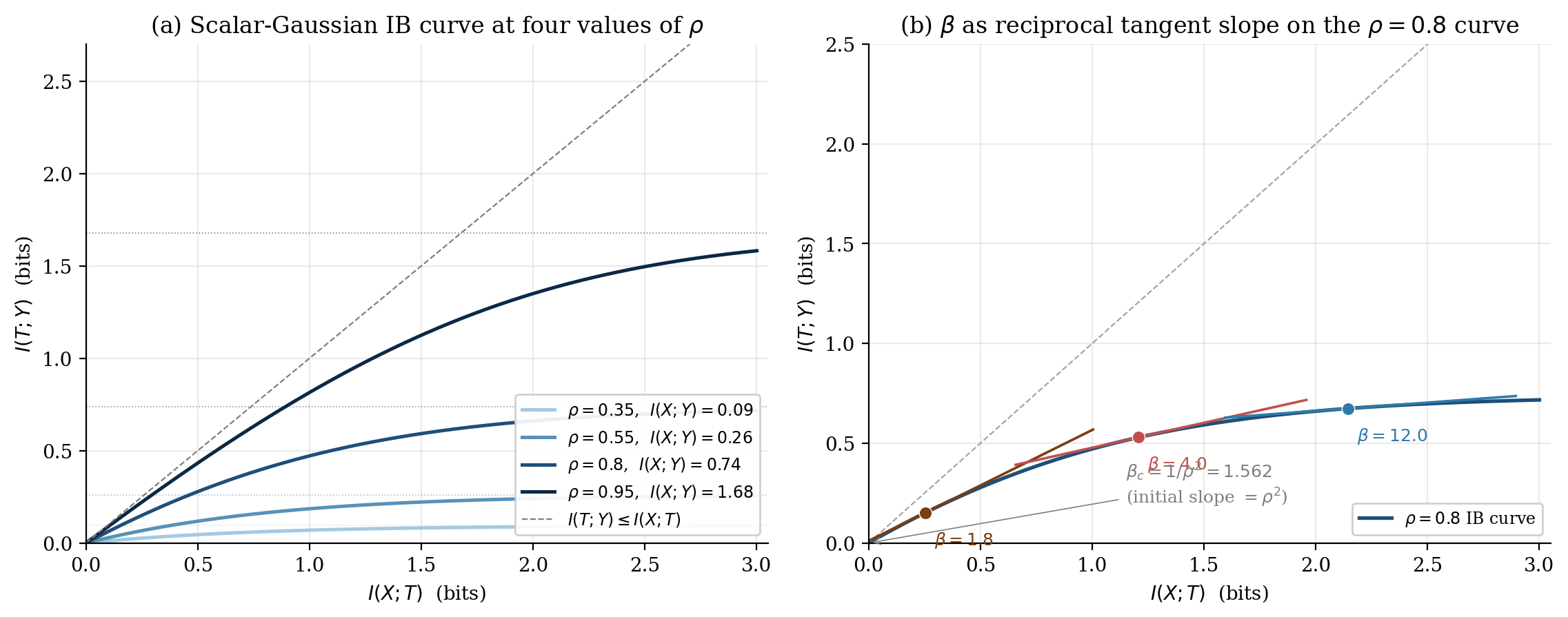
Drag β past β_c = 1/ρ² to escape the trivial encoder; the tangent line's slope is always 1/β, which is the KKT identity (2.5). At ρ = 0.8 the §2.4 reference operating points sit at (0.254, 0.152), (1.208, 0.529), and (2.145, 0.674) bits for β ∈ {1.8, 4, 12}.

This figure previews a result derived formally in §6 (the Gaussian closed form), framed for §2 as a concrete example that makes the curve shape and the $\beta$-as-slope interpretation tangible.

3. The IB fixed-point equations

3.1 Stationarity conditions on the Lagrangian

We are looking for encoders $p^*(t \mid x)$ that minimize the Lagrangian

$\mathcal{F}_\beta\bigl(p(t \mid x)\bigr) \;=\; I(X; T) - \beta\, I(T; Y) \quad\quad (3.1)$

subject to the normalization constraints $\sum_t p(t \mid x) = 1$ for every $x$. Augmenting with multipliers $\mu(x)$ gives the full Lagrangian

$\mathcal{L}_\beta \;=\; I(X; T) - \beta\, I(T; Y) + \sum_x \mu(x)\left[\sum_t p(t \mid x) - 1\right]. \quad\quad (3.2)$

At a stationary point we need $\partial \mathcal{L}_\beta / \partial p(t \mid x) = 0$ for every $(x, t)$ with $p(x) > 0$, together with the normalization constraint.

Equation (3.3) is the central formula of discrete IB. Read it as a soft-assignment rule: input $x$ is assigned to cluster $t$ with probability proportional to the cluster’s prior $p(t)$ times the exponential of $-\beta$ times the KL between the true target distribution at $x$, namely $p(y \mid x)$, and the cluster-conditional target distribution, $p(y \mid t)$. Two clusters whose target distributions are close to $p(y \mid x)$ both attract $x$; the one whose target distribution is closer wins more probability. The bandwidth of “closer wins” is set by $\beta$ — at small $\beta$ assignments are diffuse; at large $\beta$ each input goes almost entirely to its closest cluster.

The two other quantities $p(t)$ and $p(y \mid t)$ are not independent free parameters — they are determined by $p(t \mid x)$ through (2.1). So (3.3) is really a self-consistency equation: the encoder $p(t \mid x)$ defines the marginal and the decoder, which in turn feed back into the right-hand side. We will turn this self-consistency into the iterative algorithm in §3.3.

3.2 Derivation via variational calculus

We compute the two partial derivatives that show up in (3.2). Throughout we adopt the convention that $\log$ is the natural log (the conversion to bits is a global factor of $1/\ln 2$ that drops out of the stationarity condition).

The implicit-term-vanishes identity (3.9) expresses a structural feature of the IB problem: $p(y \mid t)$, viewed as a function of the encoder, is the “Bayes-optimal” estimate of $Y$ given $T = t$ averaged over the encoder’s induced distribution on $X$, so the gradient of any quantity computed from $p(y \mid t)$ that is “evaluated at its own optimal estimate” picks up no first-order correction. This is the same observation that makes EM monotone and that makes the IB algorithm Blahut–Arimoto-style monotone, which we’ll prove in §4.

3.3 The three coupled updates

A stationary point of $\mathcal{F}_\beta$ must satisfy three coupled self-consistency equations:

$$\begin{aligned} p(t \mid x) &\;=\; \frac{p(t)}{Z(x, \beta)}\, \exp\!\bigl[-\beta\, D_{\mathrm{KL}}(p(y \mid x) \,\|\, p(y \mid t))\bigr], \\[4pt] p(t) &\;=\; \sum_x p(x)\, p(t \mid x), \\[4pt] p(y \mid t) &\;=\; \frac{1}{p(t)} \sum_x p(y \mid x)\, p(x)\, p(t \mid x). \end{aligned} \quad\quad (3.13)$$

These are the IB equations. The natural way to attack a coupled fixed-point system like (3.13) is alternating substitution: hold two of the three quantities fixed, update the third, repeat. Concretely, fix some initial encoder $p^{(0)}(t \mid x)$ and iterate

$$\begin{aligned} p^{(n)}(t) &\;=\; \sum_x p(x)\, p^{(n)}(t \mid x), \\[2pt] p^{(n)}(y \mid t) &\;=\; \frac{1}{p^{(n)}(t)} \sum_x p(y \mid x)\, p(x)\, p^{(n)}(t \mid x), \\[2pt] p^{(n+1)}(t \mid x) &\;=\; \frac{p^{(n)}(t)}{Z^{(n)}(x, \beta)}\, \exp\!\bigl[-\beta\, D_{\mathrm{KL}}(p(y \mid x) \,\|\, p^{(n)}(y \mid t))\bigr]. \end{aligned} \quad\quad (3.14)$$

This is the iterative IB algorithm (Tishby, Pereira, and Bialek 1999). §4 proves that the algorithm decreases $\mathcal{F}_\beta$ monotonically and converges to a stationary point of (3.13); §5 runs it on the eight-document toy.

Three structural features of (3.13):

Labeling invariance. Permuting the cluster labels in $T$ leaves the IB equations invariant. Two clusters $t, t'$ with the same prior $p(t) = p(t')$ and the same conditional $p(y \mid t) = p(y \mid t')$ are indistinguishable — under (3.13) they will receive identical assignment probabilities from every $x$. This is the source of the bifurcation pattern in §5: clusters that are degenerate at low $\beta$ split into distinct clusters as $\beta$ crosses a phase-transition value.

The trivial fixed point. Setting $p(t \mid x) = q(t)$ (any $x$-independent distribution) makes the right-hand side of the first equation independent of $x$ as well. So the trivial encoder is always a fixed point — it is the unique fixed point for $\beta < \beta_c$, and loses stability at $\beta = \beta_c$.

The implicit data dependence. The IB equations involve $p(y \mid x)$, $p(x)$, and $p(x, y)$ only — they don’t use any external “distortion function.” This is the structural feature that distinguishes IB from rate-distortion (see §3.4).

3.4 Why these are a Blahut–Arimoto cousin

The IB iteration (3.14) inherits its template from the Blahut–Arimoto algorithm for computing rate-distortion functions (covered in rate-distortion theory). The BA algorithm minimizes the rate-distortion Lagrangian

$\mathcal{F}_s^{\mathrm{RD}}\bigl(p(\hat x \mid x)\bigr) \;=\; I(X; \hat X) + s\, \mathbb{E}\bigl[d(X, \hat X)\bigr], \qquad s > 0, \quad\quad (3.15)$

with stationarity condition

$p(\hat x \mid x) \;=\; \frac{p(\hat x)}{Z^{\mathrm{RD}}(x, s)}\, \exp\!\bigl[-s\, d(x, \hat x)\bigr]. \quad\quad (3.16)$

Compare side-by-side with the IB condition (3.3):

$p(t \mid x) \;=\; \frac{p(t)}{Z(x, \beta)}\, \exp\!\bigl[-\beta\, D_{\mathrm{KL}}(p(y \mid x) \,\|\, p(y \mid t))\bigr].$

Structurally identical. The role of the rate-distortion distortion $d(x, \hat x)$ is played in IB by

$d_{\mathrm{IB}}(x, t) \;=\; D_{\mathrm{KL}}\bigl(p(y \mid x) \,\|\, p(y \mid t)\bigr), \quad\quad (3.17)$

which we may call the predictive distortion — a measure of how badly the cluster-conditional $p(y \mid t)$ approximates the true conditional $p(y \mid x)$. Two clusters are “close” in the IB sense if they make similar predictions about $Y$, not if they look similar in input space. Compression is therefore task-aligned: it preserves bits useful for predicting $Y$ and discards everything else.

There is one crucial difference between IB and rate-distortion, however, which is the key technical reason IB is harder. In rate-distortion, the distortion $d(x, \hat x)$ is given as input — fixed before the algorithm starts. In IB, the predictive distortion $d_{\mathrm{IB}}(x, t)$ depends on $p(y \mid t)$, which depends on the encoder $p(t \mid x)$, which depends on the predictive distortion. The “distortion” emerges from the iteration itself. As a consequence:

• The rate-distortion Lagrangian $\mathcal{F}_s^{\mathrm{RD}}$ is convex in $p(\hat x \mid x)$ for fixed distortion, so BA converges to the global minimum.
• The IB Lagrangian $\mathcal{F}_\beta$ is not convex in $p(t \mid x)$, so the IB iteration converges only to a local stationary point — generally to one of many.

This non-convexity has consequences we’ll feel in §5: running the IB iteration with different random initializations finds different stationary points, and the global IB curve has to be traced by either (a) running many restarts at each $\beta$ and keeping the best, or (b) using $\beta$-annealing — solving at small $\beta$ first and warm-starting at the next $\beta$.

Despite the non-convexity, the IB iteration enjoys a clean monotonicity property — $\mathcal{F}_\beta$ decreases at every step — and convergence to a stationary point. We prove both in §4.

4. Convergence of the IB updates

4.1 The Lagrangian decreases at every step

The IB iteration (3.14) updates the encoder by a non-trivial coupled rule, so monotone decrease of $\mathcal{F}_\beta$ is not obvious from the update form alone. The clean proof goes through a wider three-argument functional — the same Csiszár–Tusnády construction that gives convergence of Blahut–Arimoto for rate-distortion and of EM for likelihood maximization.

Setup: the auxiliary functional. Treat the encoder $p(t \mid x)$, the cluster marginal $q(t)$, and the cluster decoder $r(y \mid t)$ as independent arguments. Define

$F\bigl[p, q, r\bigr] \;:=\; \sum_{x, t} p(x)\, p(t \mid x)\, \log \frac{p(t \mid x)}{q(t)} \;+\; \beta \sum_{x, t} p(x)\, p(t \mid x)\, D_{\mathrm{KL}}\bigl(p(y \mid x) \,\|\, r(y \mid t)\bigr). \quad\quad (4.1)$

The first sum looks like $I(X; T)$ but uses the auxiliary $q$ in the denominator. The second looks like the expected KL “predictive distortion” but uses the auxiliary $r$ as the cluster decoder. Both reduce to their actual-quantity versions when $q$ and $r$ equal the encoder’s induced marginal and decoder respectively.

The construction is worth lingering on: $F[p, q, r]$ is a Lyapunov-with-slack — it equals $\mathcal{F}_\beta(p)$ plus two KL-divergence penalties that vanish precisely when $q$ and $r$ are the encoder’s induced quantities. The IB iteration alternately tightens the slack and minimizes the loosened objective. This Csiszár–Tusnády pattern proves Blahut–Arimoto, EM, and CAVI convergence — IB specializes it to the predictive-KL distortion.

4.2 Boundedness and limit-point existence

Boundedness of $\mathcal{F}_\beta^{(n)}$. $I(X; T) \ge 0$ and $I(T; Y) \le I(X; Y)$ by DPI, so

$\mathcal{F}_\beta(p) \;\ge\; -\beta\, I(X; Y). \quad\quad (4.5)$

Monotone decrease plus a lower bound implies the sequence $\mathcal{F}_\beta^{(n)}$ converges to some limit $\mathcal{F}_\beta^{(\infty)}$.

Compactness. Iterates $p^{(n)}(t \mid x)$ live in the compact product of simplices $\prod_x \Delta^{|\mathcal{T}|-1}$. By Bolzano–Weierstrass, every subsequence has a convergent sub-subsequence.

Limit points are fixed points. The IB update map $\mathcal{T}_{\mathrm{IB}}$ is continuous on the simplex interior. If $p^{(n_k)} \to p^*$, then $\mathcal{T}_{\mathrm{IB}}(p^{(n_k)}) \to \mathcal{T}_{\mathrm{IB}}(p^*)$. By the equality case of Theorem 3, $p^* = \mathcal{T}_{\mathrm{IB}}(p^*)$.

4.3 What the algorithm converges to: stationary, not global

Theorems 3 and 4 give stationary-point convergence, not global-minimum convergence. Three observations.

Trivial vs nontrivial fixed points. The encoder $p(t \mid x) = q(t)$ (any $x$-independent distribution) is always a fixed point. For $\beta < \beta_c$ it is the unique fixed point and the global minimum. For $\beta > \beta_c$ the trivial fixed point becomes a saddle: small perturbations grow under iteration.

Symmetry-broken fixed points. Multiple equivalent solutions exist by cluster-label permutation — all give the same $\mathcal{F}_\beta$ value but trip up direct iterate comparisons.

Genuinely distinct local minima. Beyond labeling, the IB landscape can have multiple genuinely distinct stationary points at different $\mathcal{F}_\beta$ values. Random initialization picks between basins essentially at random.

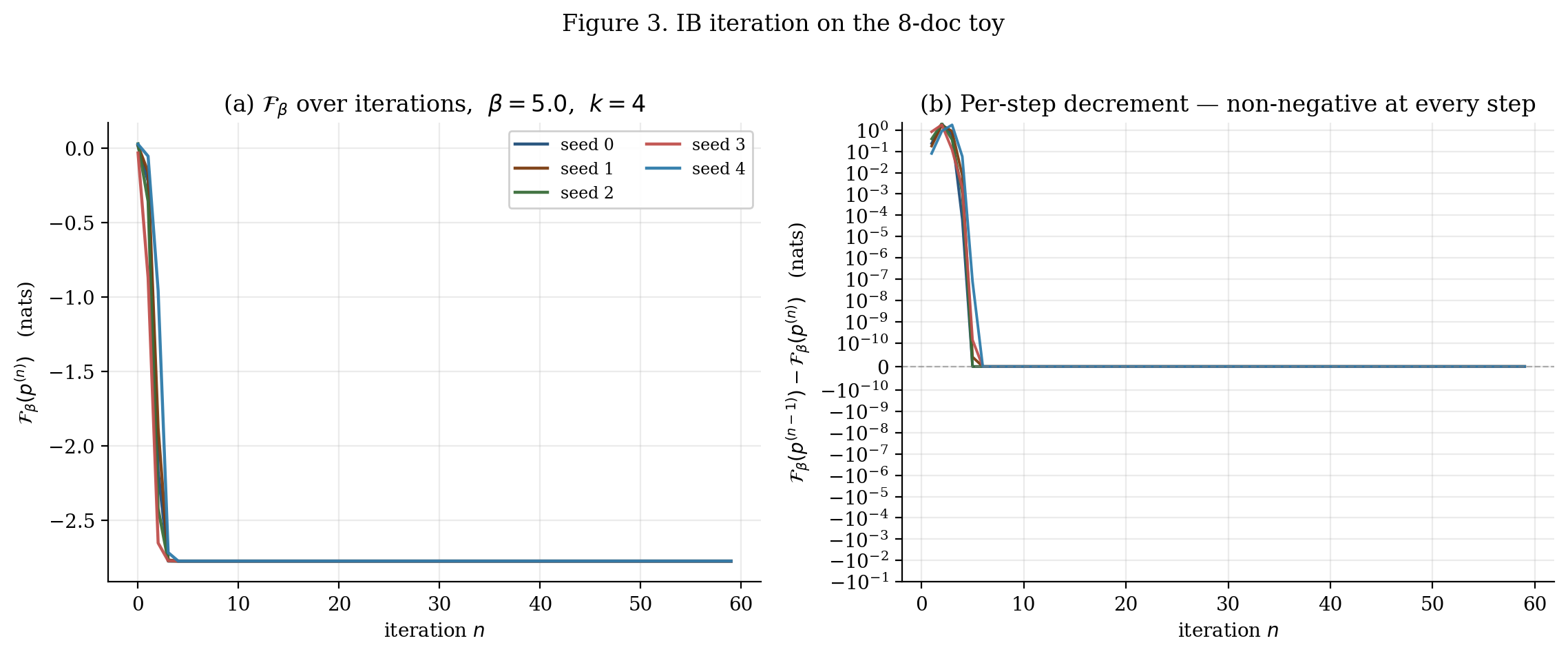
The numerical experiment in Figure 3 illustrates this: five random initializations at $\beta = 5$, $k = 4$ on the eight-document toy land at slightly different $\mathcal{F}_\beta$ values — some runs find the optimum, others get stuck.

4.4 The non-convexity hazard and annealing in β

Two practical remedies for the non-convexity exposed in Figure 3.

Random restarts. At each $\beta$ of interest, run the iteration from $M$ random initializations and keep the lowest $\mathcal{F}_\beta$ at convergence. Embarrassingly parallel. The failure mode is high $M$ — when the landscape has many basins, $M$ must scale with the number of basins.

β-annealing. Solve at a small $\beta_0$ first (where the landscape is convex, trivial encoder is the unique fixed point), then incrementally raise $\beta$, warm-starting each new $\beta$ from the previous $\beta$‘s converged encoder. The IB curve is continuous in $\beta$, so neighboring $\beta$ values have neighboring optimal encoders. Annealing traces a smooth path along the IB curve.

Annealing has a structural benefit beyond non-convexity: it makes the cluster bifurcations explicit. At small $\beta$, all clusters collapse onto the trivial fixed point. As $\beta$ crosses $\beta_c$, two clusters split apart. At larger $\beta$ thresholds, further splits occur — each phase transition activates an additional cluster. The annealing trace through the IB plane traces out the staircase of phase transitions that §5 makes visible for the discrete toy and §7 for the Gaussian closed form.

§5 implements both strategies on the eight-document toy and traces the full IB curve.

5. The discrete IB in practice

5.1 Initialization and random restarts

§4 left us with an algorithm that decreases $\mathcal{F}_\beta$ monotonically and converges to a fixed point — without guaranteeing the best fixed point. Three practical choices fill in the operational picture.

Encoder initialization. The IB iteration is a self-map on the simplex product $\prod_x \Delta^{|\mathcal{T}|-1}$. We start from a random softmax draw:

$p^{(0)}(t \mid x) \;=\; \frac{\exp\bigl(W_{x t}\bigr)}{\sum_{t'} \exp\bigl(W_{x t'}\bigr)}, \qquad W_{x t} \sim \mathcal{N}(0, \sigma^2). \quad\quad (5.1)$

Small $\sigma$ (say $\sigma \in [0.05, 0.5]$) yields a near-trivial initial encoder. The random-softmax form is easier to control numerically than near-uniform perturbations, and it keeps every cluster nonempty at initialization so that no $p^{(0)}(t) = 0$ propagates a $\log 0$ through the first update.

The escape-from-saddle problem. At any $\beta > \beta_c$, the trivial encoder $p(t \mid x) = q(t)$ is a saddle point of $\mathcal{F}_\beta$. An iterate that lands too close to it can take many iterations to escape. With $\sigma = 0$ exactly, the iteration is stationary and never moves. Always use $\sigma > 0$.

Random restarts. At each $\beta$ of interest, run from $M$ independent initializations and keep the lowest $\mathcal{F}_\beta$ at convergence. For small toys $M = 5$ to $20$ suffices.

β-annealing. Solve at a small starting $\beta_0$ first, then incrementally increase $\beta$, warm-starting each new $\beta$ from the previous $\beta$‘s converged encoder. Two practical wrinkles: (i) at each $\beta$ step, add a tiny random perturbation to the warm-start encoder to break exact saddle-point degeneracy, and (ii) the $\beta$ grid should be log-spaced and dense near suspected phase transitions to resolve their location.

From §5.3 onward: anneal forward across $\beta$ as the primary strategy, with random-restart sanity checks at selected $\beta$ to confirm we haven’t missed a lower-$\mathcal{F}_\beta$ branch.

5.2 A worked example on the eight-document toy

Before sweeping $\beta$, exhibit the algorithm on the running eight-document toy from §1.2 at fixed $\beta = 5$. Since $\beta_c = 1$ for this toy, $\beta = 5$ sits well past the first transition. With $k = 4$ clusters and random-softmax initialization at $\sigma = 0.5$, the iteration converges in roughly 17 iterations.

The trajectory has a characteristic shape: in the first few iterations, $\mathcal{F}_\beta$ drops sharply as the encoder finds the topic-aligned partition; over the next dozen iterations, $\mathcal{F}_\beta$ creeps toward its limit while the two “spare” clusters merge with the two topic clusters. By iteration 30, the per-step decrement is at machine precision.

The converged encoder uses only $\approx 2$ effective clusters (out of the 4 allocated), with the two spare clusters bleeding into the active ones. The converged $(I(X;T), I(T;Y))$ equals $(\ln 2, \ln 2) \approx (0.693, 0.693)$ nats — exactly the optimum achieved by the $T = Y$ encoder. The optimum $\mathcal{F}_\beta^* = (1 - \beta) \ln 2 = -4 \ln 2 \approx -2.7726$ nats matches the value found by four of the five seeds in Figure 3 (one seed gets stuck in a suboptimal local minimum that uses one cluster’s worth of effective capacity inefficiently).

5.3 Tracing the IB curve by sweeping β

The eight-document toy has only one phase transition because $H(Y) = 1$ bit caps the staircase. For a multi-transition example we introduce a richer toy — call it T3 for “three-topic graded purity”:

Six documents in three topics, with $p(x)$ uniform. Conditional $p(y \mid x)$ varies by document pair:

• Docs 0, 1: $p(y \mid x) = (0.85,\, 0.10,\, 0.05)$ — very topic-0 pure.
• Docs 2, 3: $p(y \mid x) = (0.10,\, 0.85,\, 0.05)$ — very topic-1 pure.
• Docs 4, 5: $p(y \mid x) = (0.15,\, 0.15,\, 0.70)$ — moderately topic-2 pure.

Three distinct conditional distributions, with the first two highly distinguishable (purity 0.85) and the third moderately distinct from the others (purity 0.70). For this construction the numerical values are $H(Y) = 1.088$ nats, $H(Y \mid X) = 0.618$ nats, hence $I(X;Y) = 0.470$ nats $(= 0.678$ bits$)$.

Setting $k = 4$ (one spare cluster to confirm self-disabling), we sweep $\beta$ across 40 log-spaced values in $[0.3,\, 100]$, annealing forward with warm-starts. The result is plotted in Figure 4: the IB curve in the $(I(X;T), I(T;Y))$ plane (left), and the same data plotted as $I(X;T)$ and $I(T;Y)$ vs $\beta$ (right). The plane plot shows the smooth, concave curve from origin to saturation; the $\beta$ plot exposes the two phase transitions as visible steepness changes — the first around $\beta \approx 4$ where the encoder starts to differentiate, and the second around $\beta \approx 11$ where the third cluster activates.

The saturation point of the curve sits at $(R^\dagger, I(X;Y)) = (\log 3,\, 0.470)$ nats $= (1.099,\, 0.470)$ nats, since 3 clusters suffice to encode a minimal sufficient statistic.

Two consistency checks. Random restarts at $\beta \in \{2,\, 5,\, 15\}$ confirm the annealing trace is the global optimum: 10 random initializations at each $\beta$ converge to within machine precision of the annealing value.

β = 19.43 (idx 29/40 · I(X;T) = 1.099 nats · I(T;Y) = 0.470 nats · K_eff = 3.78)

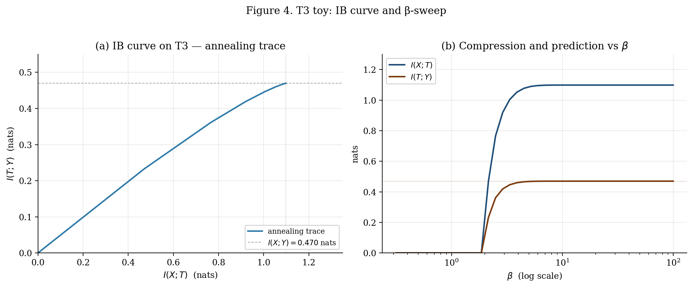
The sweep is β-annealed (each new β warm-starts from the previous β's converged encoder). Saturation point sits at (R†, I(X;Y)) = (log 3, 0.470) nats; the spare fourth cluster self-disables. Two phase transitions are visible in the right panel as steepness changes in I(T;Y).

5.4 Reading the trajectory: how clusters split with β

The IB curve in the left panel of Figure 4 is concave and continuous — phase transitions are invisible in that view. They become visible in two derived quantities, which we plot in Figure 5.

The effective cluster count. Define the perplexity of the cluster marginal:

$K_{\mathrm{eff}}(\beta) \;:=\; \exp\bigl(H(p(t))\bigr) \;=\; \exp\!\Bigl(-\!\sum_t p(t)\, \log p(t)\Bigr). \quad\quad (5.2)$

This is the “effective number of clusters” — equal to $k$ when $T$ is uniform over all $k$ clusters, equal to $1$ when $T$ collapses to a single cluster, and continuously interpolating in between when the cluster marginal is non-uniform. As $\beta$ grows, $K_{\mathrm{eff}}$ traces out a staircase: flat plateaus where the cluster structure is stable, separated by rapid climbs at the phase transitions where new clusters activate.

Cluster bifurcations as heatmaps. The right panel of Figure 5 shows the encoder $p(t \mid x)$ at four representative $\beta$ values, sampled to span the cluster-count regimes: pre-first-transition ($K_{\mathrm{eff}} \approx 1$), between transitions ($K_{\mathrm{eff}} \approx 2$), post-second-transition ($K_{\mathrm{eff}} \approx 3$), and at large $\beta$ (sharp assignments). Reading across the panels: at small $\beta$ all six documents are assigned to roughly the same cluster. At intermediate $\beta$, the encoder splits into two clusters separating docs 4–5 from the rest. At larger $\beta$, the topic-0 and topic-1 pairs separate. At very large $\beta$, the assignments are nearly one-hot — three discrete clusters, one per topic-pair.

Two structural observations. First, the order of bifurcations is not arbitrary: the first split separates the documents whose conditional distributions are most divergent. The cheapest predictive bit to encode first is the one that distinguishes the largest-divergence groups. Second, the fourth cluster we allocated self-disables: across all $\beta$, one cluster carries near-zero marginal probability $p(t) \approx 0$. IB uses only as many clusters as the structure of $p(y \mid x)$ supports.

The staircase pattern is the discrete analog of the phase transitions we will see in closed form for Gaussian IB in §7, where each canonical-correlation direction activates at a specific $\beta_c$ value determined by the spectrum.

β = 19.43 (idx 29/40 · K_eff = 3.78)

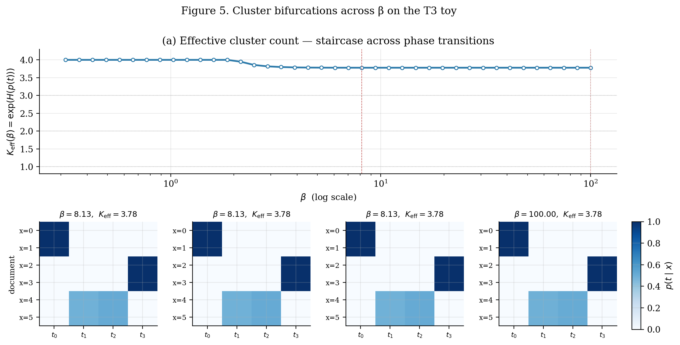
At small β, all six documents share one cluster (K_eff ≈ 1). Crossing the first phase transition splits the cluster structure — first the topic-2 pair separates from the topic-0/topic-1 group (purity 0.70 is the least correlated), then the topic-0 and topic-1 pairs separate at a higher β. The fourth allocated cluster self-disables. At large β, assignments approach one-hot and K_eff stabilizes near 3.

6. The Gaussian information bottleneck

6.1 The jointly-Gaussian setting and why it admits closed form

Through §5 the IB picture is operationally complete but every quantity is numerical. Switching to a jointly-Gaussian setting — the Chechik–Globerson–Tishby–Weiss 2005 setting — replaces iteration with matrix calculus. The Gaussian IB has a closed-form optimal encoder, an explicit expression for the IB curve as a piecewise-analytic function of $\beta$, exact locations for the phase transitions in terms of a spectrum, and a clean geometric reading via canonical-correlation analysis.

The setup. Let $X \in \mathbb{R}^p$ and $Y \in \mathbb{R}^q$ be zero-mean jointly Gaussian random vectors with covariance structure

$\Sigma_X = \mathbb{E}[X X^\top], \qquad \Sigma_Y = \mathbb{E}[Y Y^\top], \qquad \Sigma_{XY} = \mathbb{E}[X Y^\top] \in \mathbb{R}^{p \times q}. \quad\quad (6.1)$

We assume $\Sigma_X, \Sigma_Y$ are positive definite. The conditional covariance of $X$ given $Y$ has the Schur-complement form

$\Sigma_{X \mid Y} \;=\; \Sigma_X - \Sigma_{XY}\, \Sigma_Y^{-1}\, \Sigma_{YX}, \quad\quad (6.2)$

and $\Sigma_{X \mid Y} \preceq \Sigma_X$ in the positive-semidefinite order. The representation $T$ takes values in $\mathbb{R}^d$, where the dimension $d$ is determined from the spectrum below.

Why closed form is available. Two facts make the IB Lagrangian collapse to a covariance computation.

Gaussian mutual information. For jointly Gaussian $(U, V)$,

$I(U; V) \;=\; \tfrac{1}{2} \log \frac{|\Sigma_U|}{|\Sigma_{U \mid V}|}. \quad\quad (6.3)$

Mutual information depends only on second moments.

Linear-Gaussian preserves Gaussianity. If $T = A X + \xi$ where $A$ is deterministic and $\xi$ is Gaussian noise independent of $X$, then the joint $(X, T)$ and $(T, Y)$ are also jointly Gaussian. Restricting the encoder to be linear plus Gaussian noise makes the Lagrangian a function of the deterministic parameters $(A, \Sigma_\xi)$ alone.

6.2 The optimal encoder is linear plus Gaussian noise

The rigorous proof is in Chechik et al. 2005 (Theorem 1), with an entropy-power-inequality refinement in Painsky and Tishby 2017 that handles the equality cases more carefully. The intuition: for jointly-Gaussian $(X, Y)$, the predictive distortion $D_{\mathrm{KL}}(p(y \mid x) \,\|\, p(y \mid t))$ from (3.3) is the KL between two Gaussians when $T$ is also Gaussian, and that KL depends only on second moments of $(X, T, Y)$. The linear-Gaussian family spans the second-moment space, so the optimum lies in that family.

The parameterization. Standard formulas for Gaussian MI give:

$\Sigma_T \;=\; A\, \Sigma_X\, A^\top + \Sigma_\xi, \qquad \Sigma_{T \mid X} \;=\; \Sigma_\xi, \qquad \Sigma_{T \mid Y} \;=\; A\, \Sigma_{X \mid Y}\, A^\top + \Sigma_\xi. \quad\quad (6.6)$

$I(X; T) \;=\; \tfrac{1}{2} \log \frac{|A \Sigma_X A^\top + \Sigma_\xi|}{|\Sigma_\xi|}, \qquad I(T; Y) \;=\; \tfrac{1}{2} \log \frac{|A \Sigma_X A^\top + \Sigma_\xi|}{|A \Sigma_{X \mid Y} A^\top + \Sigma_\xi|}. \quad\quad (6.7)$

Combining and rearranging,

$\mathcal{F}_\beta(A, \Sigma_\xi) \;=\; \frac{1 - \beta}{2}\, \log \bigl|A \Sigma_X A^\top + \Sigma_\xi\bigr| \;+\; \frac{\beta}{2}\, \log \bigl|A \Sigma_{X \mid Y} A^\top + \Sigma_\xi\bigr| \;-\; \frac{1}{2}\, \log |\Sigma_\xi|. \quad\quad (6.8)$

Gauge freedom. The Lagrangian (6.8) is invariant under invertible linear transformations of $T$. To remove the gauge we normalize the noise covariance:

$\Sigma_\xi \;=\; I_d. \quad\quad (6.9)$

The remaining optimization is over $A \in \mathbb{R}^{d \times p}$ alone:

$\mathcal{F}_\beta(A) \;=\; \frac{1 - \beta}{2}\, \log \bigl|A \Sigma_X A^\top + I\bigr| \;+\; \frac{\beta}{2}\, \log \bigl|A \Sigma_{X \mid Y} A^\top + I\bigr|. \quad\quad (6.10)$

6.3 Reduction to a generalized eigenproblem

For symmetric $\Sigma$,

$\nabla_A \log\bigl|A \Sigma A^\top + I\bigr| \;=\; 2\,(A \Sigma A^\top + I)^{-1}\, A\, \Sigma. \quad\quad (6.11)$

Setting $\nabla_A \mathcal{F}_\beta(A) = 0$ gives

$(1 - \beta)\,(A \Sigma_X A^\top + I)^{-1}\, A\, \Sigma_X \;+\; \beta\,(A \Sigma_{X \mid Y} A^\top + I)^{-1}\, A\, \Sigma_{X \mid Y} \;=\; 0. \quad\quad (6.12)$

The diagonalization ansatz. Define

$M \;:=\; \Sigma_{X \mid Y}\, \Sigma_X^{-1} \;\in\; \mathbb{R}^{p \times p}. \quad\quad (6.13)$

$M$ has eigenvalues $\lambda_1 \le \lambda_2 \le \cdots \le \lambda_p$ in $(0, 1]$ (positive because $\Sigma_{X \mid Y}$ is PSD; at most $1$ because $\Sigma_{X \mid Y} \preceq \Sigma_X$). The right eigenvectors $v_i$ satisfy $\Sigma_{X \mid Y} v_i = \lambda_i \Sigma_X v_i$. Normalize in the $\Sigma_X$-inner-product: $v_i^\top \Sigma_X v_j = \delta_{ij}$.

Ansatz. Take

$A \;=\; \mathrm{diag}(\alpha_1, \ldots, \alpha_d)\; V^\top, \qquad V = [v_1\; v_2\; \cdots\; v_d]. \quad\quad (6.14)$

Plugging into (6.10), both $A \Sigma_X A^\top$ and $A \Sigma_{X \mid Y} A^\top$ become diagonal, and the Lagrangian decouples across directions:

$\mathcal{F}_\beta(\alpha_1, \ldots, \alpha_d) \;=\; \sum_{i=1}^d \biggl[\frac{1 - \beta}{2}\, \log(1 + \alpha_i^2) \;+\; \frac{\beta}{2}\, \log(1 + \alpha_i^2 \lambda_i)\biggr]. \quad\quad (6.15)$

Setting $u_i := \alpha_i^2$ and $\partial \mathcal{F}_\beta / \partial u_i = 0$,

$u_i^* \;=\; \alpha_i^{*\,2} \;=\; \frac{\beta(1 - \lambda_i) - 1}{\lambda_i}, \quad\quad (6.16)$

provided the right-hand side is non-negative — i.e., $\beta > 1/(1 - \lambda_i)$. Otherwise the directional minimum is at $\alpha_i^* = 0$ and direction $i$ is inactive.

Ansatz optimality. Is the diagonal-in-eigenbasis form (6.14) optimal among all $A$? Yes — by the von Neumann trace inequality applied to the simultaneous diagonalization of $\Sigma_X$ and $\Sigma_{X \mid Y}$ in the $\Sigma_X$-inner-product basis $\{v_i\}$. See Chechik et al. 2005 (Lemma 3.2) for the detailed argument.

Summary. The optimal Gaussian-IB encoder at $\beta$ is

$A^*_\beta \;=\; \mathrm{diag}(\alpha_1^*, \ldots, \alpha_d^*)\, V_d^\top, \qquad \alpha_i^{*\,2} \;=\; \max\!\biggl(0,\; \frac{\beta(1 - \lambda_i) - 1}{\lambda_i}\biggr), \quad\quad (6.17)$

where $V_d$ holds the $d$ smallest-eigenvalue eigenvectors of $M$. Each direction switches on at the critical

$\beta_{c,\, i} \;=\; \frac{1}{1 - \lambda_i}. \quad\quad (6.18)$

6.4 Reading the canonical-correlation spectrum

The eigenvalues $\lambda_i$ of $M = \Sigma_{X \mid Y}\, \Sigma_X^{-1}$ measure the fraction of $X$‘s variance unexplained by $Y$. $\lambda_i \to 1$ means direction $v_i$ is uncorrelated with $Y$; $\lambda_i \to 0$ means direction $v_i$ is strongly determined by $Y$.

Canonical correlations. The eigenvalues of $M$ are related to the canonical correlations between $X$ and $Y$:

$\lambda_i \;=\; 1 - \rho_i^2, \quad\quad (6.19)$

where $\rho_1 \ge \rho_2 \ge \cdots$ are the canonical correlations (sorted descending), with $\rho_i \in [0, 1]$. Substituting into (6.18):

$\beta_{c,\, i} \;=\; \frac{1}{\rho_i^2}. \quad\quad (6.20)$

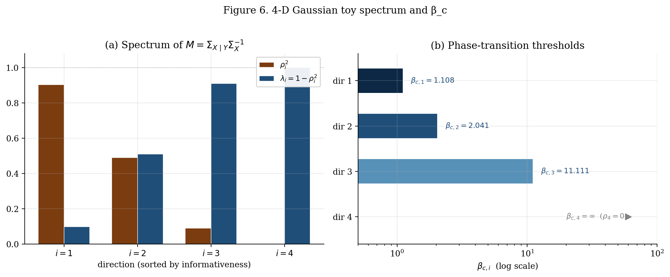
The IB phase transitions happen at the reciprocals of the squared canonical correlations, in order of decreasing $\rho_i$. The most-correlated direction activates first; $\rho_i = 0$ directions never activate. The IB algorithm finds exactly the CCA directions, in order of statistical informativeness — the same projections Hotelling 1936 derived from a correlation-maximization argument, here motivated by predictive compression instead.

The 4-D toy. We build a synthetic 4-D jointly-Gaussian example with designed canonical correlations $\rho = (0.95,\, 0.70,\, 0.30,\, 0)$. Each $\rho_i$ encodes a different “informativeness regime.” The phase-transition staircase comes out:

• $\beta < 1.108$: trivial encoder, $T = \text{const}$.
• $1.108 < \beta < 2.041$: one active direction $(\rho_1 = 0.95)$.
• $2.041 < \beta < 11.111$: two active directions.
• $\beta > 11.111$: three active directions; the fourth never activates.

The total $I(X;Y) = -\tfrac{1}{2}\sum_i \log(1 - \rho_i^2) = 1.548$ nats. A Monte Carlo verification with $n = 50{,}000$ samples recovers the canonical correlations to within $|\hat\rho - \rho| \le 0.0023$.

7. Phase transitions on the Gaussian IB curve

7.1 Critical β values determined by the spectrum

From §6, the optimal Gaussian-IB encoder at parameter $\beta$ is given by (6.17) with thresholds $\beta_{c, i} = 1/(1 - \lambda_i) = 1/\rho_i^2$. Sorting eigenvalues ascending gives an ordered sequence

$\beta_{c,\, 1} \;<\; \beta_{c,\, 2} \;<\; \cdots \;<\; \beta_{c,\, r}, \quad\quad (7.1)$

where $r = \mathrm{rank}(\Sigma_{XY})$. Directions with $\rho_i = 0$ never activate.

The first phase transition is at $\beta_{c, 1}$, not at $\beta = 1$. For general jointly Gaussian $(X, Y)$, the first transition is the inverse of the largest squared canonical correlation, which is in $(0, 1]$. So $\beta_{c, 1} \ge 1$ always, with equality iff $X$ and $Y$ share a perfectly correlated direction.

The activation order is by canonical correlation, not by the original coordinates. The CCA directions $v_i$ are linear combinations of the original components of $X$; they need not align with any coordinate axis. The IB principle is coordinate-free: it sees only the second-moment structure of $(X, Y)$, expressed through $\rho_1, \rho_2, \ldots$.

7.2 Closed-form curve and the C¹-but-not-C² distinction

Plugging (6.17) into (6.7) uses two algebraic identities:

$1 + \alpha_i^{*\,2} \;=\; \frac{(\beta - 1)(1 - \lambda_i)}{\lambda_i}, \qquad 1 + \alpha_i^{*\,2}\, \lambda_i \;=\; \beta\,(1 - \lambda_i). \quad\quad (7.2)$

For each active direction $i$:

$I(X; T_\beta)_i \;=\; \tfrac{1}{2} \log \!\biggl(\frac{(\beta - 1)(1 - \lambda_i)}{\lambda_i}\biggr), \quad\quad (7.3)$

$I(T_\beta; Y)_i \;=\; \tfrac{1}{2} \log \!\biggl(\frac{\beta - 1}{\beta\, \lambda_i}\biggr). \quad\quad (7.4)$

Summing over all active directions $i$ at parameter $\beta$:

$I(X; T_\beta) \;=\; \frac{1}{2} \sum_{i:\, \beta > \beta_{c,\, i}} \log\!\biggl(\frac{(\beta - 1)(1 - \lambda_i)}{\lambda_i}\biggr), \qquad I(T_\beta; Y) \;=\; \frac{1}{2} \sum_{i:\, \beta > \beta_{c,\, i}} \log\!\biggl(\frac{\beta - 1}{\beta\, \lambda_i}\biggr). \quad\quad (7.5)$

The IB curve is piecewise analytic in $\beta$: across each open interval $(\beta_{c,\, k},\, \beta_{c,\, k+1})$, exactly $k$ directions are active. At each phase transition, the activating direction contributes zero exactly at the threshold, so the curve is continuous in $\beta$.

The slope $dI(T;Y) / dI(X;T) = 1/\beta$ at every interior point. Differentiating (7.3) and (7.4):

$\frac{dI(X; T_\beta)_i}{d\beta} \;=\; \frac{1}{2\,(\beta - 1)}, \qquad \frac{dI(T_\beta; Y)_i}{d\beta} \;=\; \frac{1}{2\,\beta\,(\beta - 1)}. \quad\quad (7.6)$

The ratio is $1/\beta$ per direction. Summing over $k$ active directions multiplies both by $k$, leaving the ratio unchanged. The IB curve has tangent slope $1/\beta$ at every interior point, recovering (2.5).

Curvature jumps at each phase transition. From the chain rule and (7.6),

$\frac{d^2 I(T;Y)}{d I(X;T)^2} \;=\; -\frac{2\,(\beta - 1)}{k\,\beta^2}. \quad\quad (7.7)$

At each $\beta_{c,\, k+1}$, the curvature magnitude decreases by a factor of $k/(k+1)$ — the curve becomes less curved when a new direction activates. The IB curve is $C^1$ but not $C^2$: the tangent is everywhere continuous (slope $1/\beta$ on both sides of each transition), but the curvature jumps. This is why phase transitions are invisible in a smooth-looking plot of $I(T;Y)$ against $I(X;T)$ yet very visible in the $\beta$-parameterization: in the IB plane they show up only as a faint curvature change, while in the $\beta$-plot they are sharp kinks in the activation timing.

Saturation. As $\beta \to \infty$, $I(T_\beta; Y)_i$ saturates at $-\tfrac{1}{2}\, \log \lambda_i$ per active direction. Total:

$\lim_{\beta \to \infty} I(T_\beta; Y) \;=\; -\frac{1}{2} \sum_{i:\, \rho_i > 0} \log \lambda_i \;=\; -\frac{1}{2} \log \frac{|\Sigma_{X \mid Y}|}{|\Sigma_X|} \;=\; I(X; Y), \quad\quad (7.8)$

recovering the DPI ceiling exactly.

7.3 Dimension allocation: how each new direction turns on

The closed form decomposes $I(X; T_\beta)$ and $I(T_\beta; Y)$ by canonical-correlation direction, and that decomposition is plotted as a stacked area in Figure 8.

Activation is staged. Below $\beta_{c,\, 1}$, all bands are flat at zero. At each $\beta_{c,\, i}$, direction $i$‘s band starts climbing from zero.

Within an active region, contributions are unequal. For two simultaneously-active directions $i, j$:

$I(T;Y)_i \;-\; I(T;Y)_j \;=\; \tfrac{1}{2}\, \log(\lambda_j / \lambda_i),$

constant in $\beta$ once both are active. The IB doesn’t rebalance — it adds new directions while preserving the existing ordering between them.

Most-correlated direction dominates. For the 4-D toy:

• Direction 1 $(\rho_1 = 0.95)$: saturation $-\tfrac{1}{2}\log(0.0975) \approx 1.164$ nats — 75.2% of $I(X;Y)$.
• Direction 2 $(\rho_2 = 0.70)$: $\approx 0.337$ nats — 21.8%.
• Direction 3 $(\rho_3 = 0.30)$: $\approx 0.047$ nats — 3.0%.
• Direction 4: 0 (never activates).

This is the Gaussian-IB analog of “dominant principal component” in PCA, with one substantive difference: PCA ranks directions by $X$-variance; Gaussian IB ranks them by predictiveness of $Y$.

β = 20.00 (3 active directions · I(X;T) = 4.352 nats · I(T;Y) = 1.471 nats)

dir 1: ρ = 0.95, λ = 0.098, β_c = 1.11

dir 2: ρ = 0.70, λ = 0.510, β_c = 2.04

dir 3: ρ = 0.30, λ = 0.910, β_c = 11.11

dir 4: ρ = 0.00, λ = 1.000, β_c = ∞

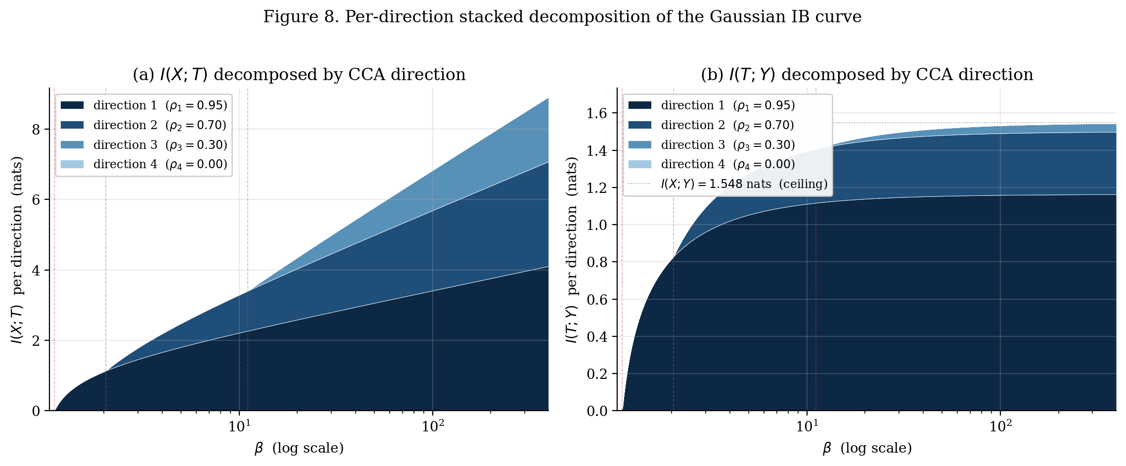
Direction 1 dominates the predictiveness budget: it saturates at −½ log λ_1 ≈ 1.164 nats (75.2% of I(X;Y)). Direction 2 contributes ≈ 0.337 nats (21.8%), direction 3 ≈ 0.047 nats (3.0%). Direction 4 (ρ_4 = 0) never activates.

7.4 Numerical verification on a 4-D toy

We check (7.3)–(7.5) by Monte Carlo. Protocol:

1. Sample $(X, Y)$ from the joint Gaussian designed in §6.4.
2. For each $\beta \in \{1.5,\, 2.5,\, 5.0,\, 15.0\}$, construct $A^*_\beta$ and sample $T = A^*_\beta X + \xi$.
3. Compute empirical $I(X; T)$ and $I(T; Y)$ using the Gaussian-MI formula on the empirical covariances.
4. Compare to the closed-form values from (7.5).

The four β land in different active-direction regimes — β = 1.5 (one active direction), 2.5 (two), 5.0 (two), 15.0 (three). Closed-form values, in nats:

β	I(X;T) (cf)	I(T;Y) (cf)
1.5	0.7661	0.6146
2.5	1.4981	0.9898
5.0	2.4789	1.2775
15.0	3.8944	1.4443

At $n_{\text{MC}} = 20{,}000$ samples, agreement is within $O(1/\sqrt{n}) \approx 10^{-2}$ nats — confirming both the encoder construction and (7.5) at once. The notebook prints the side-by-side comparison; max-abs-difference across the four β is below $6 \times 10^{-3}$ nats.

β = 5.00 (I(X;T) = 2.479 nats · I(T;Y) = 1.277 nats · 2 active directions)

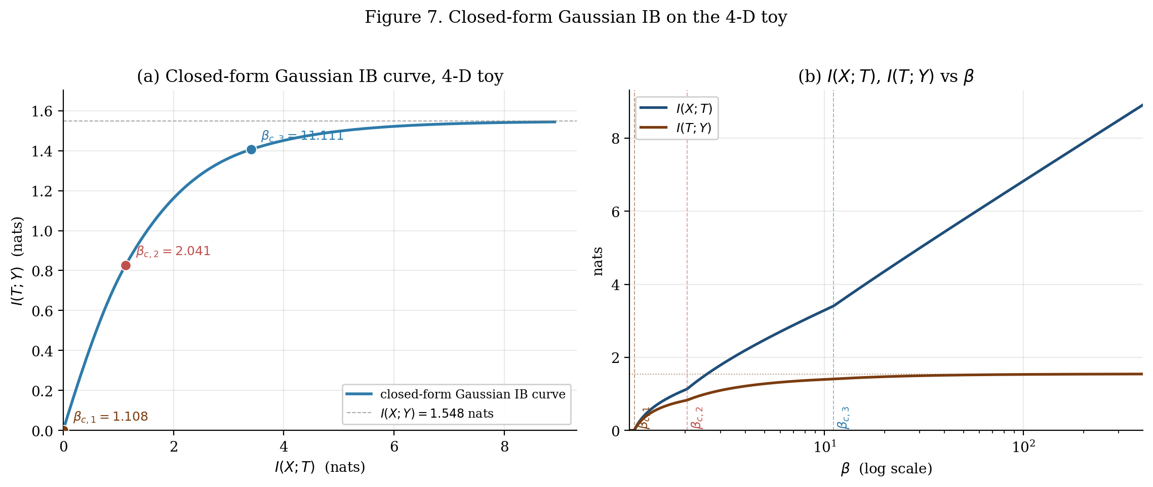
Phase transitions at β_c = (1.108, 2.041, 11.111) activate the three nonzero canonical-correlation directions. The fourth (ρ_4 = 0) never activates. Saturation at I(X;Y) = 1.548 nats. Try β = 1.5 → (0.766, 0.615), β = 2.5 → (1.498, 0.990), β = 5.0 → (2.479, 1.278), β = 15 → (3.894, 1.444) — the four §7.4 verification points.

8. Variational IB and the deep-learning lift

8.1 Why direct IB doesn’t scale to high-dimensional encoders

The §3 IB algorithm has two requirements that limit its reach in practice. First, every iteration uses the conditional $p(y \mid x)$ at every $x$ — that means we need the whole joint distribution $p(x, y)$ as input. Second, the encoder $p(t \mid x)$ is represented explicitly for every $x$. Both requirements break down when $X$ is high-dimensional continuous data.

We need two structural changes. First, amortize the encoder: instead of storing $p(t \mid x)$ for every $x$, parameterize it by a neural network $p_\theta(t \mid x)$ whose parameters $\theta$ are shared across $x$. Second, upper-bound the intractable terms in the IB Lagrangian by quantities estimable from samples.

This is what Alemi, Fischer, Dillon, and Murphy did in 2017, building on Achille and Soatto (information dropout), Kingma and Welling (VAE), and Tishby–Zaslavsky. The result, Variational Information Bottleneck (VIB), is the workhorse of the IB-in-deep-learning literature.

8.2 The Alemi–Fischer–Dillon–Murphy 2017 variational bound

Upper bound on $I(X; T)$. For any auxiliary distribution $q(t)$ over $\mathcal{T}$,

$I(X; T) \;=\; \mathbb{E}_x\bigl[D_{\mathrm{KL}}(p(t \mid x) \,\|\, q(t))\bigr] \;-\; D_{\mathrm{KL}}(p(t) \,\|\, q(t)) \;\le\; \mathbb{E}_x\bigl[D_{\mathrm{KL}}(p(t \mid x) \,\|\, q(t))\bigr], \quad\quad (8.1)$

with equality iff $q(t) = p(t)$. The practical choice — for tractability and for connecting to the VAE — is $q(t) = \mathcal{N}(0, I)$.

Lower bound on $I(T; Y)$. For any auxiliary $r(y \mid t)$,

$I(T; Y) \;\ge\; \mathbb{E}_{(t, y)}\bigl[\log r(y \mid t)\bigr] \;+\; H(Y), \quad\quad (8.2)$

with equality iff $r(y \mid t) = p(y \mid t)$.

Combining. The VIB upper bound on $\mathcal{F}_\beta$ (absorbing constants) is

$\mathcal{L}_{\mathrm{VIB}}\bigl(p_\theta, q, r_\phi\bigr) \;:=\; \mathbb{E}_x\bigl[D_{\mathrm{KL}}(p_\theta(t \mid x) \,\|\, q(t))\bigr] \;-\; \beta\, \mathbb{E}_{(x, y, t)}\bigl[\log r_\phi(y \mid t)\bigr]. \quad\quad (8.3)$

Compare to (3.1): same two-term structure (rate $+ \beta$-weighted distortion), but each term is now a bound rather than the exact MI.

Connection to the ELBO. Equation (8.3) is structurally identical to the negative variational evidence lower bound for a supervised latent-variable model: encoder $p_\theta(t \mid x)$, prior $q(t)$, decoder $r_\phi(y \mid t)$. VIB is VAE with the targets switched — instead of reconstructing $X$, predict $Y$. This identification (Alemi et al. 2017, §3) unlocked the full deep-learning toolkit for IB.

When is the bound tight? With $q$ free: $q = p(t)$. With $r$ free: $r = p(y \mid t)$. In practice $q$ is fixed at $\mathcal{N}(0, I)$, so the bound is strictly loose. The gap is $D_{\mathrm{KL}}(p_\theta(t) \,\|\, q(t))$ — the KL between the encoder’s induced marginal and the chosen prior. This becomes a regularization that pulls the encoder toward producing a Gaussian-marginal $T$.

8.3 Amortized encoders and the reparametrization trick

Diagonal-Gaussian amortized encoder. Parameterize

$p_\theta(t \mid x) \;=\; \mathcal{N}\bigl(t;\, \mu_\theta(x),\, \mathrm{diag}\bigl(\sigma_\theta^2(x)\bigr)\bigr), \quad\quad (8.4)$

with $\mu_\theta(x), \sigma_\theta(x) \in \mathbb{R}^d$ neural-network outputs sharing parameters across all $x$.

Reparametrization (Kingma and Welling 2014). Sampling $t \sim p_\theta(t \mid x)$ is differentiable in $\theta$ via

$t \;=\; \mu_\theta(x) \,+\, \sigma_\theta(x) \odot \epsilon, \qquad \epsilon \sim \mathcal{N}(0, I). \quad\quad (8.5)$

Stochasticity lives in $\epsilon$, independent of $\theta$ — gradients pass straight through.

Minibatch SGD. For dataset $\{(x_n, y_n)\}_{n=1}^N$,

$\widehat{\mathcal{L}}_{\mathrm{VIB}}(\theta, \phi) \;=\; \frac{1}{N} \sum_{n=1}^N \Bigl[D_{\mathrm{KL}}(p_\theta(t \mid x_n) \,\|\, q(t)) \;-\; \beta\, \mathbb{E}_{\epsilon}[\log r_\phi(y_n \mid \mu_\theta(x_n) + \sigma_\theta(x_n) \odot \epsilon)]\Bigr]. \quad\quad (8.6)$

The VIB training loop is almost identical to a VAE training loop, with one substitution: the decoder predicts $Y$ from $T$ instead of $X$ from $T$. Code-wise, switching from VAE to VIB is a one-line change.

8.4 A closed-form linear-Gaussian VIB sandbox

To pull the VIB framework off the SGD treadmill, restrict to the linear-Gaussian case: jointly Gaussian $(X, Y)$ from §6 setup, Gaussian encoder $p_\theta(t \mid x) = \mathcal{N}(A x, \Sigma_\xi)$, fixed Gaussian prior $q(t) = \mathcal{N}(0, I)$, and Gaussian decoder $r_\phi(y \mid t) = \mathcal{N}(B t, \Sigma_\eta)$.

Closed-form objective. Expanding (8.3):

$\mathcal{L}_{\mathrm{VIB}}(A, \Sigma_\xi, B, \Sigma_\eta) \;=\; \tfrac{1}{2}\bigl[\mathrm{tr}(\Sigma_T) - \log|\Sigma_\xi| - d\bigr] \;+\; \tfrac{\beta}{2}\, \mathrm{NLL}(B, \Sigma_\eta;\, A, \Sigma_\xi), \quad\quad (8.7)$

where $\Sigma_T = A \Sigma_X A^\top + \Sigma_\xi$. The optimal decoder is $B^* = \Sigma_{YX}\, A^\top\, \Sigma_T^{-1}$ and $\Sigma_\eta^* = \Sigma_{Y \mid T}$. After this inner optimization,

$\mathcal{L}_{\mathrm{VIB}}^*(A, \Sigma_\xi) \;=\; \underbrace{\tfrac{1}{2}\bigl[\mathrm{tr}(\Sigma_T) - \log|\Sigma_\xi| - d\bigr]}_{\text{rate (upper bound on } I(X;T) \text{)}} \;+\; \underbrace{\tfrac{\beta}{2}\, \log\bigl|\Sigma_Y - \Sigma_{YX}\, A^\top\, \Sigma_T^{-1}\, A\, \Sigma_{XY}\bigr|}_{\text{distortion (lower bound on } -I(T;Y) \text{)}}. \quad\quad (8.8)$

Gap to the true IB Lagrangian. The rate term overshoots $I(X; T)$ by exactly

$D_{\mathrm{KL}}\bigl(\mathcal{N}(0,\, \Sigma_T) \,\|\, \mathcal{N}(0,\, I)\bigr), \quad\quad (8.9)$

the KL from the encoder’s induced marginal to the unit-Gaussian prior. The gap vanishes only when $\Sigma_T = I$, which is generally not the IB optimum’s marginal.

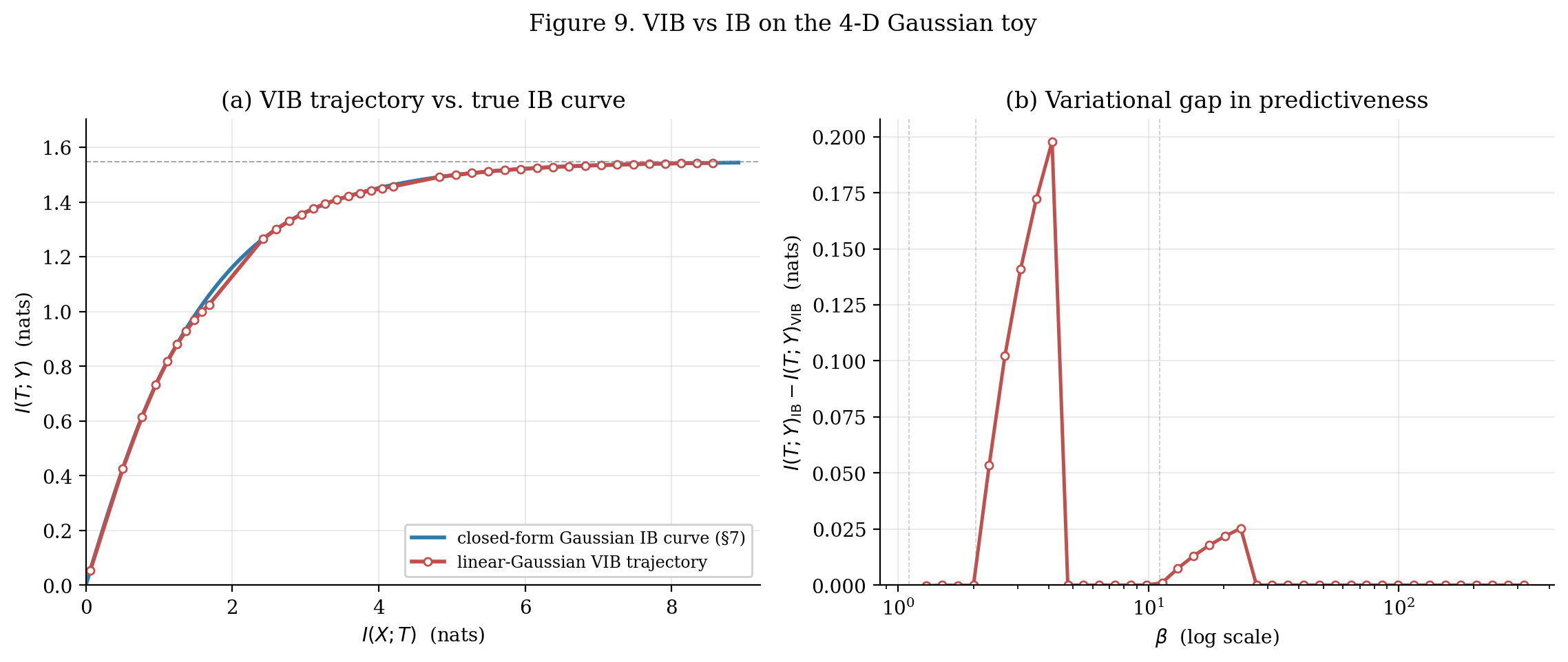
Numerical experiment. Optimize (8.8) over $(A, \Sigma_\xi)$ at 40 log-spaced $\beta$ on the 4-D toy from §6.4 with L-BFGS-B and $\beta$-annealing warm-starts. At each $\beta$, compute the actual $(I(X;T), I(T;Y))$ using §6’s closed-form Gaussian MI formulas — this evaluates the bound’s tightness, not its self-consistency.

The result: VIB trajectory traces a curve that stays inside (below and right of) the true IB curve, with the gap visible across all $\beta$. At small $\beta$ the gap is small (both near origin); at intermediate $\beta$ the gap is largest; at large $\beta$ both saturate at $I(T;Y) = I(X;Y)$.

Loading VIB precompute (40 L-BFGS-B optima)…

9. The fitting and compression controversy

9.1 The Tishby–Zaslavsky and Shwartz-Ziv–Tishby claim

The most-discussed application of the IB principle in deep learning has been a descriptive one: the claim that deep networks, when trained by SGD, traverse a characteristic trajectory in the information plane that explains why they generalize. Tishby and Zaslavsky proposed this picture in 2015; Shwartz-Ziv and Tishby formalized and experimentally documented it in 2017.

For a feedforward classifier with hidden layers $T_1, T_2, \ldots, T_L$, estimate $I(X; T_l)$ and $I(T_l; Y)$ from the training data each epoch and plot trajectories. Shwartz-Ziv and Tishby (on tanh-activated networks) observed every layer’s trajectory tracing two phases:

The fitting phase. Early in training, $I(X; T_l)$ and $I(T_l; Y)$ both grow. Diagonal climb in the IB plane.

The compression phase. Later in training, $I(T_l; Y)$ stays high while $I(X; T_l)$ decreases. Leftward bend in the plane. Interpretation: late-phase SGD performs a diffusion in weight space that compresses the representations.

Three claims rode this picture:

1. Compression is generic. Predicted for any deep classifier trained by SGD.
2. Compression explains generalization. Late SGD performs implicit IB-style regularization.
3. Deep nets implicitly do IB. Slogan packaging of (1) + (2).

The picture was provocative, visually compelling, and immediately influential. It also turned out to be contested.

9.2 The information-plane visualization

Setting aside the interpretive claims, the visualization — $(I(X; T_l),\, I(T_l; Y))$ over training — is a legitimate tool. Its catch is that computing it requires an MI estimator for high-dimensional continuous $T$.

Binning. Discretize $T$, plug-in. Sensitive to bin width and saturating activations.

$k$-NN-based (Kraskov–Stögbauer–Grassberger 2004). Principled, slow, biased in high dimensions.

Parametric / variational. Fit a model. Tractable when correctly specified; biased when not.

The choice of estimator can change the qualitative shape of the trajectory. This is the methodological wedge that Saxe et al. drove into the original picture.

9.3 Saxe et al. 2018: tanh vs ReLU and the compression artifact

Saxe, Bansal, Dapello, Advani, Kolchinsky, Tracey, and Cox (ICLR 2018) ran the experiment with two variations the original work hadn’t probed.

Activation function. Shwartz-Ziv–Tishby used tanh; Saxe et al. replicated with ReLU. With tanh, compression appeared; with ReLU, the compression phase disappeared. $I(X; T_l)$ grew monotonically throughout. Same architecture, same training, same dataset — qualitatively different trajectories depending on activation.

MI estimator artifact. Tanh activations saturate near $\pm 1$. During training, activation values cluster into the boundary bins. The binning estimator interprets this as information loss even though no real information has been lost. With ReLU (no saturation), no such clustering.

Analytical sandbox. Saxe et al. analyzed linear networks where MI is computable in closed form. In the linear-Gaussian setting, SGD shows no compression phase. This was the cleanest evidence that compression is not intrinsic to SGD on deep nets.

Their conclusion. The compression phase in the original experiments is artifactual — an interaction between tanh’s saturation and the binning estimator. Switch to ReLU or to closed-form MI, and the phase disappears. The two-phase trajectory is not a generic feature of SGD on deep networks.

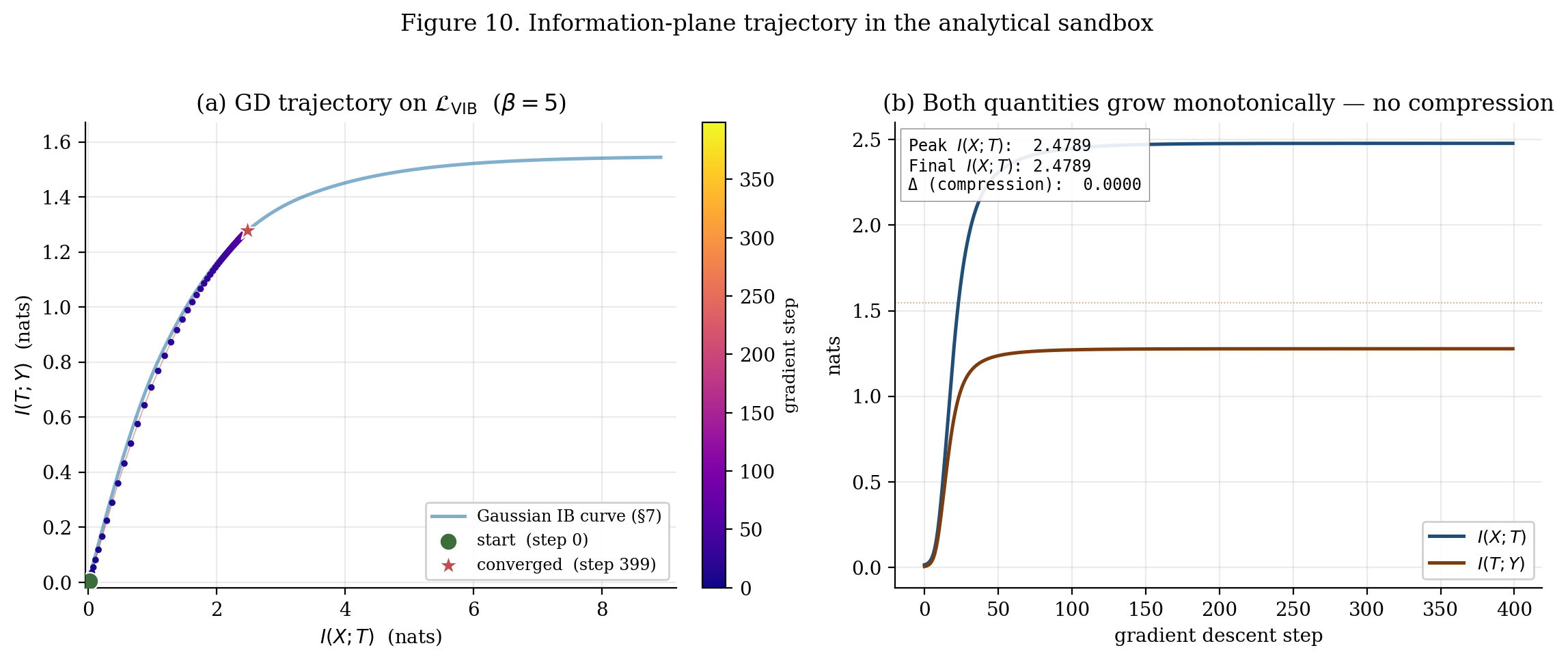
A short demonstration of the analytical case appears in Figure 10. We run gradient descent on the closed-form linear-Gaussian VIB objective from §8 at fixed $\beta = 5$, track the trajectory using the exact Gaussian MI formulas (no estimator), and observe: $I(X; T)$ and $I(T; Y)$ both grow monotonically. There is no compression phase. The “compression delta” — peak $I(X;T)$ minus final $I(X;T)$ — comes out to $0.0000$ nats on this run.

9.4 What the controversy leaves intact (and what it doesn’t)

What did not survive Saxe et al. 2018 and the work that followed:

• The claim that compression is a generic feature of SGD on deep networks.
• The claim that compression explains deep-network generalization.
• The packaging “deep learning is information bottleneck.”

What did survive:

• The information plane as a visualization tool. Plotting $(I(X; T_l), I(T_l; Y))$ over training remains useful for understanding what a network’s hidden representations are doing, with the caveat that the MI estimator matters.
• VIB as a regularizer. Alemi et al.’s MNIST experiments showed measurable robustness gains against adversarial examples, independent of any descriptive claim about implicit IB in unmodified SGD.
• The fitting phase. Uncontroversially observed by everyone.
• Compression as an inducible phenomenon. Saturating activations, stochastic noise injection (Achille and Soatto’s Information Dropout), explicit IB regularization (VIB) — all produce compression on purpose. Not automatic, but a useful design choice.

Goldfeld, van den Berg, Greenewald, Melnyk, Nguyen, Kingsbury, and Polyanskiy (NeurIPS 2019) showed that compression is closely tied to entropic regularization of the activations — either via discretization, or via injected noise. Compression observed in the information plane is real when it appears, but it appears as a consequence of specific structural choices, not as a universal SGD phenomenon.

Honest assessment. The IB principle is most useful held as a prescriptive Lagrangian rather than a descriptive theory of deep learning. The prescriptive reading (VIB, Information Dropout) is well-founded and has measurable benefits. The descriptive reading (deep nets implicitly do IB) was overreached and has been substantially walked back. The framework is sharp in its proper domain — clear $X$, clear $Y$, the need for a compressed $T$ that retains predictiveness — and weaker the further one pushes it past that domain.

10. IB beyond compression-vs-prediction

The IB Lagrangian’s two-term structure generalizes naturally to multi-term variants by adding mutual-information quantities with their own Lagrange multipliers. Three application stories illustrate this modularity.

10.1 Information dropout and the emergence of invariance

Achille and Soatto (2018) implement VIB via a multiplicative-noise injection on activations:

$T \;=\; f(W X) \,\odot\, \exp(Z), \qquad Z \sim \mathcal{N}\bigl(0,\, \sigma_\theta^2(X)\bigr), \quad\quad (10.1)$

with $\sigma_\theta(X)$ a learned, input-dependent noise scale. For ReLU activations, (10.1) implements a log-normal noise on the positive part of $T$. The objective is the VIB Lagrangian (8.3) with a log-normal prior.

The invariance claim. A representation $T$ is invariant to a nuisance factor $N$ when $T \perp N \mid Y$. Achille and Soatto show that minimizing the VIB Lagrangian with sufficient $\beta$ produces representations whose $X$-content is exactly the part of $X$ that predicts $Y$. Nuisances are squeezed out by the compression term. Invariance is a consequence of IB compression, not an extra ingredient.

The disentanglement claim. Under information dropout, components of $T$ become approximately independent conditional on $Y$, more sharply at higher $\beta$. The IB Lagrangian’s $\beta$ is, structurally, the $\beta$-VAE’s $\beta$ (Higgins et al. 2017) — they are the same quantity in different applications.

What the framing buys. Information dropout gives a one-line architectural change (multiplicative noise on activations) that implements VIB-style regularization. The IB principle used prescriptively — as a design tool — produces invariance and partial disentanglement automatically.

10.2 IB framings of fair representation learning

Moyer, Gao, Brekelmans, Galstyan, and Ver Steeg (2018) cast fair representation learning as a generalized IB problem with an explicit sensitive-attribute penalty.

Setup. $X$ is the input, $Y$ the prediction target, $S$ a sensitive attribute. The goal: $T$ that predicts $Y$ well, contains minimal info about $S$, and stays compact about $X$. The fair-IB Lagrangian:

$\mathcal{L}_{\mathrm{fair}}\bigl(p(t \mid x)\bigr) \;=\; \underbrace{I(X; T)}_{\text{rate}} \;-\; \underbrace{\beta_Y\, I(T; Y)}_{\text{utility}} \;+\; \underbrace{\beta_S\, I(T; S)}_{\text{leakage}}, \quad\quad (10.2)$

with two Lagrange multipliers controlling utility and leakage. The Pareto frontier sweeps a three-axis trade-off.

Variational treatment. Each MI term gets a variational bound following §8: upper bound on $I(X;T)$ via $\mathbb{E}[D_{\mathrm{KL}}(p(t \mid x) \,\|\, q(t))]$, lower bound on $I(T;Y)$ via an auxiliary decoder $r_Y$, upper bound on $I(T;S)$ via a second auxiliary decoder $r_S$. End-to-end trainable by SGD.

Comparison to adversarial fair-rep. The pre-Moyer-et-al. approach was adversarial: learn $T$ alongside a discriminator $D_S$, train $T$ to fool $D_S$. Minimax, GAN-style, training instability. The IB approach bounds $I(T;S)$ directly via its variational form — single-level minimization, no minimax. Empirically (UCI Adult, Heritage Health), IB matches or beats adversarial fair-rep with more stable training.

What the framing buys. Each new constraint is one variational term plus one $\beta$. Single-level optimization, end-to-end differentiable.

10.3 IB framings of privacy and the utility–leakage trade-off

Replace the sensitive attribute $S$ with all of the information we want to protect:

$\mathcal{L}_{\mathrm{priv}}\bigl(p(t \mid x)\bigr) \;=\; -\, I(T; Y) \;+\; \beta_S\, I(T; S), \quad\quad (10.3)$

(or with $X$ in the leakage slot for full anonymization).

Connection to differential privacy. DP gives worst-case guarantees (bounded $\log p(T \mid D)/p(T \mid D')$ for adjacent datasets); IB-privacy gives average-case guarantees (bounded $I(T; X)$ or $I(T; S)$). DP is stronger and has composition theorems; IB-privacy is more flexible — it produces a Pareto frontier rather than a single budget.

Operational interpretation. Issa, Wagner, and Kamath (2020) showed that $I(T; S)$ has a clean operational meaning: it is the expected log-ratio by which a Bayesian adversary’s posterior on $S$ improves after observing $T$. Minimizing $I(T; S)$ is literally minimizing the expected information gain an adversary obtains.

Practical use cases. Federated learning, synthetic data generation, selective-attribute privacy. The deep-learning machinery (VIB encoders, decoders, reparametrization) transfers directly.

A unifying observation. Each application here is one instance of a multi-term IB Lagrangian:

Application	Rate	Predictiveness	Other
Standard IB / VIB	$I(X;T)$	$\beta\, I(T;Y)$	—
Information dropout	$I(X;T)$ via mult. noise	$\beta\, I(T;Y)$	—
Fair-rep (Moyer et al.)	$I(X;T)$	$\beta_Y\, I(T;Y)$	$\beta_S\, I(T;S)$ leakage
Privacy	$I(X;T)$ anonymization	$\beta\, I(T;Y)$ utility	$\beta_S\, I(T;S)$ leakage

§11 places this template in its broader context.

11. Connections to other principles

11.1 IB and rate-distortion: the same Lagrangian template

The classical rate-distortion Lagrangian for source $X$ with distortion $d$:

$\mathcal{F}_s^{\mathrm{RD}}\bigl(p(\hat x \mid x)\bigr) \;=\; I(X; \widehat{X}) \;+\; s\, \mathbb{E}\bigl[d(X, \widehat{X})\bigr], \qquad s \ge 0. \quad\quad (11.1)$

The IB Lagrangian rewritten:

$\mathcal{F}_\beta\bigl(p(t \mid x)\bigr) \;=\; I(X; T) \;+\; \beta\, \bigl[I(X;Y) - I(T;Y)\bigr] \;-\; \beta\, I(X;Y). \quad\quad (11.2)$

IB is rate-distortion with the predictive distortion:

$d_{\mathrm{IB}}(X, T) \;=\; D_{\mathrm{KL}}\bigl(p(y \mid X) \,\|\, p(y \mid T)\bigr), \qquad \mathbb{E}[d_{\mathrm{IB}}(X, T)] \;=\; I(X;Y) - I(T;Y). \quad\quad (11.3)$

Where they differ. RD’s distortion is fixed before the algorithm runs. IB’s distortion depends on the encoder iterate through the induced $p(y \mid t)$. Two consequences:

1. RD Lagrangian is convex in $p(\hat x \mid x)$ for fixed distortion → BA converges globally. IB is not convex → BA finds local stationary points.
2. R(D) admits closed forms. Gaussian RD has $R(D) = \tfrac{1}{2} \log(\sigma^2 / D)$. Gaussian IB has a closed-form curve (§7) with a different distortion. Both curves are convex-decreasing.

Side-by-side numerical comparison at common rates and $\rho = 0.9$:

R (nats)	RD: $D = e^{-2R}$	IB: $D_{\mathrm{pred}}$
0.20	0.6703	0.6750
0.50	0.3679	0.4716
1.00	0.1353	0.2277
2.00	0.0183	0.0376

The IB distortion is larger at every rate — the price of using a self-emergent distortion that depends on $Y$ rather than a fixed Euclidean one.

Correlation ρ = 0.90 (I(X;Y) = 0.830 nats — the IB saturation rate)

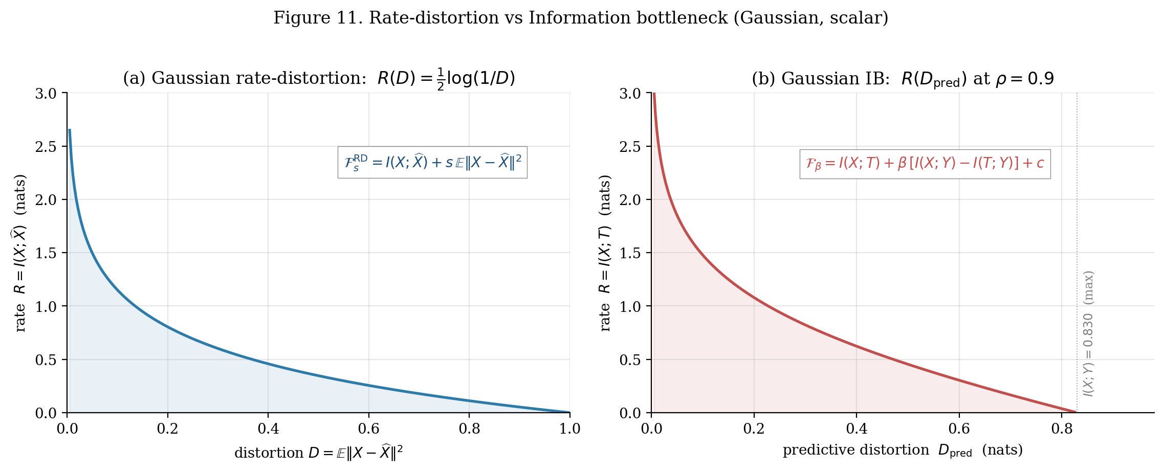
Both curves are convex decreasing in (D, R) — structurally identical shape. The substantive difference is the distortion's provenance: RD takes d(X, X̂) as input, fixed before the algorithm runs; IB derives D_pred = D_KL(p(y|x) ‖ p(y|t)) from the encoder iterate itself. The side-by-side at ρ = 0.9 reproduces the brief's §11.1 table: at R = 0.20, RD has D ≈ 0.670 vs IB D_pred ≈ 0.675; at R = 2.00, RD ≈ 0.018 vs IB ≈ 0.038.

The full rate-distortion theory is developed in rate-distortion; §11.1 here just makes the structural parallel explicit.

11.2 IB and PAC-Bayes: KL as a complexity penalty

PAC-Bayes (McAllester 1999; Catoni 2007) bounds generalization for stochastic learners. With probability $\ge 1 - \delta$ over draws of training set $S$:

$\mathbb{E}_{h \sim Q}\bigl[L(h)\bigr] \;\le\; \mathbb{E}_{h \sim Q}\bigl[\widehat{L}_S(h)\bigr] \;+\; \sqrt{\frac{D_{\mathrm{KL}}(Q \,\|\, P) + \log(1 / \delta)}{2 n}}, \quad\quad (11.4)$

where $Q$ is the data-conditional posterior and $P$ is a data-independent prior. The KL term is a complexity penalty.

Structural parallel with IB. The IB rate $I(X; T) = \mathbb{E}_x[D_{\mathrm{KL}}(p(t \mid x) \,\|\, p(t))]$ is a KL between a data-conditional encoder and its marginal. PAC-Bayes’s $D_{\mathrm{KL}}(Q \,\|\, P)$ is structurally analogous.

Russo–Zou / Xu–Raginsky. Russo and Zou (2016) and Xu and Raginsky (2017) gave a tight information-theoretic generalization bound: for stochastic algorithm $p(S, A)$ with sub-Gaussian loss,

$\bigl|\mathbb{E}\bigl[L(A) - \widehat{L}_S(A)\bigr]\bigr| \;\le\; \sqrt{\frac{2\, \sigma^2\, I(S; A)}{n}}. \quad\quad (11.5)$

The generalization gap is bounded by the mutual information between training set and learned hypothesis.

The unifying picture. A stochastic learning rule whose output depends only weakly on the input (in MI/KL terms) generalizes well. IB says the same thing for stochastic encoders. Same arithmetic, three framings. For VIB: bounding $I(X; T)$ during training literally controls a generalization gap, in the Russo–Zou–Xu–Raginsky sense.

11.3 IB and InfoNCE / contrastive learning

InfoNCE (van den Oord, Li, and Vinyals 2018) is the loss behind modern self-supervised representation learning. For positive pairs $(x_i, y_i)$ and $K - 1$ negatives,

$\mathcal{L}_{\mathrm{InfoNCE}}(\theta) \;=\; -\, \mathbb{E}\!\left[\log \frac{e^{f_\theta(x_i, y_i)}}{\frac{1}{K}\sum_{j = 1}^K e^{f_\theta(x_i, y_j)}}\right]. \quad\quad (11.6)$

The MI lower bound. For the optimal-discriminator score,

$I(X; Y) \;\ge\; \log K \;-\; \mathcal{L}_{\mathrm{InfoNCE}}(\theta^*). \quad\quad (11.7)$

Minimizing InfoNCE maximizes a tractable lower bound on $I(X; Y)$. Modern contrastive methods scale $K$ aggressively (SimCLR: 8192-sample batches; MoCo: even larger via momentum queues) to tighten this bound.

Connection to IB. Casting contrastive in IB notation: $X$ first view, $Y$ second view, $T = g_\theta(X)$ the representation. Contrastive learning maximizes a lower bound on $I(T; Y)$ — the predictiveness term in the IB Lagrangian.

What is missing: the compression term $I(X; T)$. Contrastive learning has no explicit rate penalty. The compression that emerges comes from the limited capacity of the representation (typically 128–256-dim projection heads). The bottleneck is structural rather than information-theoretic.

This makes contrastive learning a partial IB — the predictiveness half with architectural compression. Saunshi et al. (2019) closed the loop, showing that contrastive learning produces representations with downstream-classification generalization bounds structurally similar to PAC-Bayes-style bounds.

11.4 IB and the minimal sufficient statistic

The classical notion of sufficient statistic (Fisher 1922; Lehmann–Scheffé 1950) is the statistical-inference grandparent of IB.

Classical definition. A statistic $T = T(X)$ is sufficient for $Y$ given $X$ if $p(x \mid t)$ does not depend on $Y$ — equivalently, $I(T; Y) = I(X; Y)$. A statistic is minimal sufficient if it is sufficient and is a function of every other sufficient statistic.

The classical concept is binary. Sufficient or not. No continuous “how sufficient” scale.

IB makes sufficiency continuous. As $\beta \to \infty$, the IB optimum approaches the minimal sufficient statistic: $\lim_{\beta \to \infty} I(T_\beta^*; Y) = I(X; Y)$, and among sufficient statistics, the IB $\beta = \infty$ optimum has the smallest $I(X; T)$. The IB problem at finite $\beta$ is the lossy version of the classical sufficient-statistic problem, with $\beta$ as the lossiness knob.

This generalizes-the-classical the same way rate-distortion generalizes Shannon source coding:

Classical	Modern lossy version
Shannon source coding (lossless)	Rate-distortion
Sufficient statistic (classical)	Information bottleneck

Exponential-family sufficiency. For exponential-family $p(y \mid x) = h(y) \exp(\eta(x)^\top T_0(y) - A(\eta(x)))$, the natural parameter $\eta(X)$ is a finite-dimensional sufficient statistic. IB applied to such families produces finite-dimensional representations — the algorithm rediscovers the exponential-family structure. In the Gaussian case (§6), this is exact: the IB optimum at $\beta = \infty$ recovers the canonical-correlation projection, which is the linear-Gaussian minimal sufficient statistic.

The lineage.

Year	Contribution	Author(s)
1922	Sufficient statistics	Fisher
1948	Mutual information / source coding	Shannon
1950	Minimal sufficient statistics	Lehmann, Scheffé
1959	Rate-distortion theory	Shannon
1972	Blahut–Arimoto algorithm	Blahut; Arimoto (independently)
1999	Information bottleneck	Tishby, Pereira, Bialek
2005	Gaussian IB	Chechik, Globerson, Tishby, Weiss
2017	Variational IB	Alemi, Fischer, Dillon, Murphy

IB is, in this lineage, a 1999 modern reframing of a 1922 classical idea via Shannon’s information theory.

12. Computational notes and honest limits

12.1 Numerical stability of the IB updates

The IB iteration involves three operations that lose precision in standard float64, especially at large $\beta$. Implementing in log-space throughout is the fix.

Issue 1: the exponential. (3.3) involves $\exp(-\beta\, D_{\mathrm{KL}})$ which underflows when $\beta\, D_{\mathrm{KL}} > 700$. Use log-space:

$\log p^{(n+1)}(t \mid x) \;=\; \log p^{(n)}(t) - \beta\, D_{\mathrm{KL}}\bigl(p(y \mid x) \,\|\, p^{(n)}(y \mid t)\bigr) - \log Z(x, \beta), \quad\quad (12.1)$

with $\log Z(x, \beta) = \mathrm{logsumexp}_t[\log p^{(n)}(t) - \beta\, D_{\mathrm{KL}}]$ via scipy.special.logsumexp (or a hand-rolled max-stable version in TS).

Issue 2: zero-probability components. Extinct clusters during annealing have $p(t) = 0$; $\log 0 = -\infty$ propagates NaN. Clip: $\log p(t) \to \log \max(p(t),\, 10^{-300})$.

Issue 3: KL with vanishing summand. Use scipy.special.rel_entr(p, q) instead of computing $p \log(p / q)$ by hand. rel_entr returns $0$ when $p = 0$ and $+\infty$ when $p > 0,\, q = 0$.

Issue 4: convergence test. Compare $\mathcal{F}_\beta$ values, not encoders. Encoder distance is misleading near phase transitions where the cluster labeling can flip. Use relative-decrement $|\mathcal{F}_\beta^{(n)} - \mathcal{F}_\beta^{(n+1)}| < \epsilon \cdot |\mathcal{F}_\beta^{(n)}|$.

Implementation rule. Track $\log p(t \mid x), \log p(t), \log p(y \mid t)$ throughout. Carry out KLs, normalizations, marginalizations in log-space. Convert to probabilities only at final output. This is what the §5 viz components do — see T3IBCurveTracer.tsx and ClusterBifurcationCascade.tsx in the source.

12.2 Estimating MI on continuous data: plug-in pitfalls

The discrete IB algorithm assumed access to the joint $p(x, y)$. For continuous high-dimensional data — images, text, audio — we have samples. Every estimator has pathologies.

Binning (plug-in). Bias: positive (Roulston 1999) and bin-count-dependent. The Saxe et al. 2018 critique of Shwartz-Ziv–Tishby (§9.3) hinged on this — tanh saturation clusters activations into bins, dropping binned MI without any real information loss.

$k$-NN (Kraskov–Stögbauer–Grassberger 2004). $O(N \log N)$ per estimate; substantial negative bias in high dimensions (Belghazi et al. 2018); sensitive to $k$.

Variational bounds. MINE (Belghazi et al. 2018), InfoNCE (van den Oord et al. 2018). Training-time friendly, differentiable, scalable. Tightness depends on critic capacity; reliably tracks changes in MI; absolute values biased.

Recommendation.

Task	Estimator
Exploratory analysis, small data	$k$-NN
Training-time optimization (VIB and descendants)	Variational bounds
Descriptive claims about a network’s information plane	Be very careful — see Goldfeld et al. 2019 for guidance

12.3 Within-formalML siblings and forward pointers

Direct prerequisites.

• Shannon entropy — entropy, MI, source-coding interpretation.
• KL divergence — Pinsker, log-sum, conditioning identities.
• Rate-distortion theory — closest parent. BA-algorithm template inherited.

Soft prerequisites and structural cousins.

• Variational inference — §8.2’s bound is the same construction as the VAE ELBO.
• Representation learning — the geometric / contrastive counterpoint to IB.
• PAC-Bayes bounds — the generalization-bound family that IB’s rate term parallels.

Forward pointers.

• Bayesian neural networks — VIB as supervised Bayesian deep learning.
• Density-ratio estimation — InfoNCE = noise-contrastive density-ratio estimator.
• Normalizing flows — natural deeper-encoder family for VIB.
• Meta-learning — IB-style task representations (Achille et al. 2019).

12.4 Honest limits — what IB doesn’t tell you

1. IB doesn’t predict generalization in deep nets. The §9 controversy. The original “deep learning is IB” framing did not survive Saxe et al. Used prescriptively (VIB, Information Dropout), the framework has measurable transfer and robustness benefits; descriptively, it does not explain what SGD on unmodified networks is doing.

2. IB doesn’t tell you the optimal $\beta$ a priori. The Lagrange multiplier is application-dependent. No general procedure to pick “the right $\beta$” from data alone. In practice: cross-validate downstream performance, or target a specific rate or predictiveness.

3. IB requires either the joint $p(x, y)$ or a viable variational bound. For finite high-dim samples, neither is unproblematic. VIB’s bounds are loose by design — the encoder’s induced marginal is forced toward the prior, a deviation from the true IB optimum (§8.4 exhibited this on the Gaussian sandbox).

4. Non-uniqueness. Labeling degeneracy and genuinely distinct basins. Annealing helps; doesn’t eliminate. See Figure 3 for an explicit example on the 8-document toy.

5. The compression-prediction framing isn’t always the right one. Transfer learning across many tasks, pure self-supervised learning, learned-loss problems all push outside strict IB. Sometimes multi-constraint IB (§10) is the answer; sometimes a different framework.

6. Sample-complexity guarantees are weak. Russo–Zou / Xu–Raginsky (§11.2) gives MI-based generalization bounds, rarely tight in practice. VIB models typically outperform the bound; the gap is active research (Achille and Soatto 2018).

A closing thought. The IB principle is most useful held as a prescriptive Lagrangian rather than a descriptive theory of deep learning. It compresses, it predicts, and it has clean closed-form structure in the Gaussian setting that anchors intuition for general cases. Within its domain — clear $X$, clear $Y$, the need for a compressed $T$ that retains predictiveness — the IB and its variational descendants are sharp tools.