Always-Valid Inference
Time-uniform confidence sequences, e-processes, and the betting reformulation — sequential A/B testing without peeking penalties
1. Motivation — why fixed- confidence intervals fail under peeking
1.1 The peeking analyst
Picture an A/B test. We’ve decided to run it for 10,000 visitors, and we’ll form a 95% confidence interval for the lift at the end. After 1,000 visitors, we glance at the dashboard. The lift looks significant — the 95% CI excludes zero. We stop.
That action — peeking and stopping based on what we saw — quietly invalidates our confidence statement. The fixed- CI we relied on, say a Hoeffding band
promises exactly one thing:
That guarantee says nothing about holding simultaneously. The naïve union bound is vacuous for . We need a different kind of object — one whose coverage guarantee survives looking, deciding, and stopping.
1.2 A concrete optional-stopping demonstration
We’ll make this visceral. Generate i.i.d. — true mean . At each , form the fixed- Gaussian CI with . Adopt the aggressive-analyst stopping rule
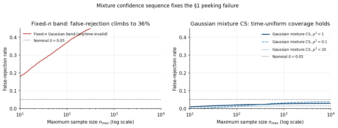
Across Monte Carlo replicates, the fraction of replicates stopping at some with the CI excluding the truth climbs from at to at , and would approach as . Drag the slider below to watch the failure rate grow with the analyst’s patience.
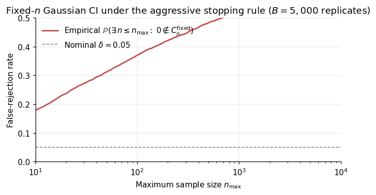
The pathology is not subtle. The fixed- band shrinks like , but fluctuates on the same scale by the CLT — so the band is exactly tight enough at any single and not tight enough to hold over all simultaneously.
1.3 The law of the iterated logarithm — a preview
The deepest reason the fixed- band fails under peeking comes from the law of the iterated logarithm (LIL), proved in Hartman and Wintner (1941) and sharpened by Strassen (1964). For i.i.d. mean-zero with variance , the partial sums satisfy
Translated to the running mean, infinitely often exceeds — a width that grows by a factor of over the fixed- band. The random walk revisits arbitrarily large -scaled deviations forever. Any band whose half-width is alone is eventually exited with probability one. The peeking analyst is a victim not of bad luck but of the law of large numbers’ fine print.
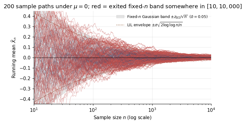
The LIL also tells us what kind of widening we’ll have to pay. Any honest confidence sequence must accommodate at least a factor. The modern boundaries of §§5–6 hit this rate up to constants; the formal discussion of the LIL as a lower bound is in §13.3.
1.4 What we want — time-uniform coverage
Definition 1.1 (Confidence sequence).
Let be a stochastic process adapted to a filtration , and let be a parameter of the data-generating distribution. A -confidence sequence for is a sequence of -measurable random sets satisfying
The “for all ” is the entire game. It promises that the event “every contains ” has probability — a statement about the full sample path, not about any individual .
Proposition 1.2 (Stopping-time equivalence).
is a -confidence sequence if and only if for every stopping time (taking values in ),
Proof.
() Fix a stopping time . On , there exists at least one finite index at which . Hence , and taking probabilities gives by (1.1).
() Define the exit time (with if no such ). Each is -measurable, so is a stopping time. On , by definition, so
by (1.2). Taking complements yields (1.1).
∎Time-uniform coverage and stopping-time validity are the same property. We use anytime-valid and time-uniform interchangeably, and say a procedure is anytime-valid if its guarantee holds under (1.2) for every stopping time, including stopping rules the analyst designs by staring at the data.
1.5 Roadmap
Arc A — Classical sequential analysis (§§3–4). Wald (1945, 1947) and Robbins (1970): the SPRT prototype and the method-of-mixtures structural template.
Arc B — Modern confidence sequences (§§5–6). Howard, Ramdas, McAuliffe, and Sekhon (2020, 2021): every fixed- Chernoff-style tail bound has a time-uniform analogue obtained by replacing Markov on the MGF with Ville on the supermartingale. Waudby-Smith and Ramdas (2024): the betting reformulation, with empirical-Bernstein confidence sequences matching LIL.
Arc C — e-values and e-processes (§§8–10). Vovk (1993, 2019), Vovk and Wang (2021), Grünwald, de Heide, and Koolen (2024): the formal definition of e-value, the duality between e-processes and anytime-valid tests, and the merging operations that handle multiple-testing without Bonferroni.
All three arcs reduce to the same one tool: Ville’s inequality applied to a nonnegative supermartingale. We develop that tool in §2.
2. From Markov to Ville — the supermartingale lift
We promised in §1 that the entire topic rests on one tool. This section delivers it. The fixed- Chernoff recipe — every tail bound on the reader has ever seen — comes from a single application of Markov’s inequality to a moment-generating function. The time-uniform version comes from a single substitution: replace that Markov step with Ville’s inequality, applied to the corresponding nonnegative supermartingale. The bounds are uniformly valid over all sample sizes simultaneously, at the cost of a factor that §13.3 will show is unavoidable.
2.1 Markov’s inequality and the fixed- Chernoff recipe
Lemma 2.1 (Markov's inequality).
For any nonnegative random variable and any ,
Markov bounds a tail probability by an expectation. The Chernoff recipe takes for some tilt :
Apply this to for i.i.d. with cumulant generating function . Independence factors the expectation, so , and Markov gives
Minimize over to get the Chernoff bound; specialize to get every named tail bound.
Example 1 (The sub-Gaussian case).
A random variable with mean is sub-Gaussian with variance proxy if for all . Plugging into (2.2), . Minimum over at equals . Inverting at level gives the fixed- Hoeffding CI
This is the band that failed under peeking in §1. It fails because the Markov step in (2.2) is a single- statement. To control the supremum over , we need an inequality that handles every at once.
2.2 Nonnegative supermartingales and Ville’s inequality
Definition 2.2 (Filtration, supermartingale).
A filtration on a probability space is an increasing sequence of -algebras , with for all . A real-valued process adapted to is a supermartingale if for all and
The supermartingale is nonnegative if almost surely for every .
Example 2 (The sub-Gaussian supermartingale).
For i.i.d. mean-zero sub-Gaussian with variance proxy , fix and define
Each trivially. The supermartingale property holds:
by the sub-Gaussian MGF bound. This is the Wald–Doob supermartingale — the canonical fixed- → time-uniform lift.
Theorem 2.3 (Ville's inequality (Ville 1939)).
Let be a nonnegative supermartingale with . Then for any ,
Same right-hand side as Markov (2.1), but the left-hand side controls the supremum of the process — every simultaneously. The same Markov budget buys a uniform statement over the whole sample path.
Proof.
We use Doob’s optional-stopping theorem for bounded stopping times (Theorem 2.5 below). Fix and define (with if no such ).
Each indicator is -measurable, so — making a stopping time. For any finite horizon , , so Theorem 2.5 gives .
On , and . On , . Hence
so , i.e. .
The events are increasing with union . Continuity of measure gives
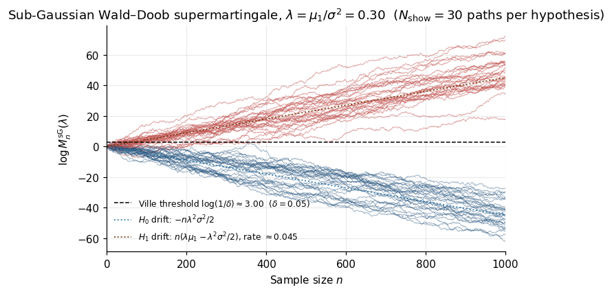
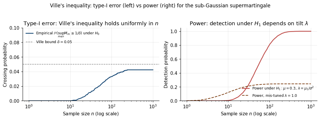
∎Empirical max crossing: H₀ = 0.039, H₁ = 1.000.
2.3 Doob’s optional-stopping theorem and stopping-time invariance
Definition 2.4 (Stopping time).
A random variable is a stopping time with respect to if for every .
The event “we’ve stopped by time ” is decidable from the first observations alone — no peeking into the future.
Theorem 2.5 (Doob's optional-stopping theorem (bounded stopping times)).
Let be a supermartingale and a stopping time with almost surely for some finite . Then
Proof.
The key combinatorial identity: for any ,
For , the indicators are for and otherwise, so the sum telescopes to . Taking expectations and using ,
by the supermartingale property. Summing over gives .
∎For unbounded the statement still holds for nonnegative supermartingales: — the uniform-integrability extension. We won’t need the unbounded version directly.
Corollary 2.6 (Stopping-time invariance of nonnegative supermartingales).
Let be a nonnegative supermartingale with . Then for any stopping time and any ,
Compare (2.8) with Proposition 1.2. Both characterize the property “guarantee holds for every stopping rule”. This is the structural reason supermartingales give anytime-valid inference.
2.4 The fixed- → time-uniform recipe
Step 1 — start with a fixed- Chernoff bound. Identify a class of distributions and an MGF upper bound such that for .
Step 2 — construct the Wald–Doob supermartingale. , , is a nonnegative supermartingale by Example 2.
Step 3 — apply Ville. , or equivalently
Step 4 — mix over to get an adaptive boundary. Replace the single- bound with for a mixing distribution . By Fubini, is a nonnegative supermartingale. Ville applies, giving the method-of-mixtures boundary of Robbins (1970).
This cookbook drives §§3–6. Every confidence sequence is steps 1–4 instantiated with a different MGF bound and mixing distribution.
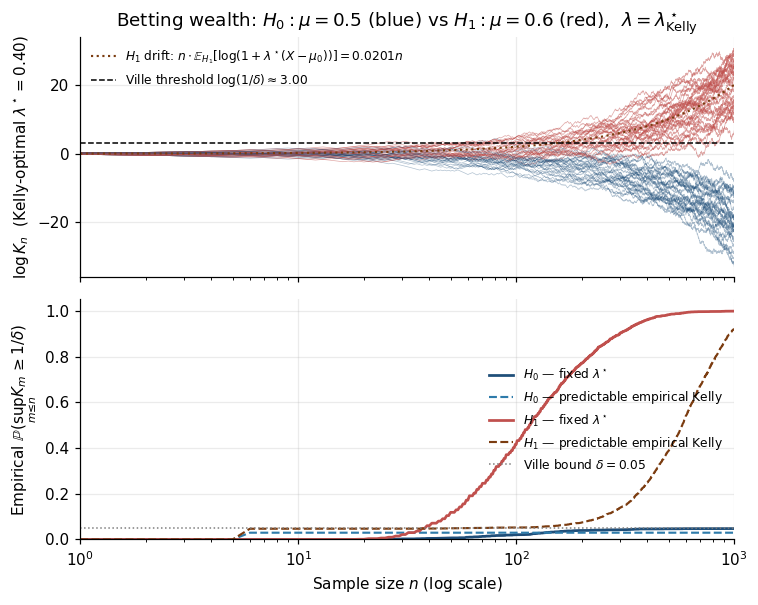
We close by validating the recipe numerically. Under , trajectories stay bounded by Ville. Under , exhibits linear positive drift , maximized at , giving the optimal log-growth — exactly the KL divergence between and . This is the first glimpse of the growth-rate-optimal property of §9.
3. The sequential probability ratio test (SPRT)
§2’s recipe is more easily appreciated through its first historical instance: Abraham Wald’s sequential probability ratio test, developed at Columbia’s Statistical Research Group in 1943 for wartime munitions inspection and declassified in Wald (1945, 1947). The SPRT is the prototype anytime-valid procedure — its statistic is a martingale under the null, Ville’s inequality gives the type-I error guarantee, and Wald’s identity gives the expected stopping time. The whole modern theory of e-processes is, structurally, the SPRT’s likelihood ratio reinterpreted as a betting wealth and generalized beyond simple-vs-simple testing.
3.1 Wald’s likelihood-ratio martingale
The SPRT addresses the simple-vs-simple hypothesis test vs for known densities. Wald’s central object is the likelihood ratio
Read as the betting odds in favor of after seeing . The logarithm turns this into a sum, with .
Lemma 3.1 (Likelihood-ratio martingale).
Let be densities with respect to , with on the support of . For i.i.d. and , is a nonnegative martingale with .
Proof.
Nonnegativity is automatic. For the martingale property,
Induction with closes the argument.
∎That this is a martingale (equality, not inequality) is the cleanest possible setup for the time-uniform lift.
Example 3 (Gaussian mean shift).
For and ,
Under , . Under , .
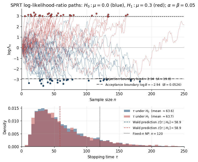
The SPRT chooses two thresholds and defines
with decision: reject if , accept if .
3.2 Boundary-crossing analysis and Wald’s identity
Type-I error. By Lemma 3.1 and Ville (Theorem 2.3),
Type-II error. The dual process is a nonnegative martingale under . Ville again:
Setting and controls both errors. Wald’s tighter approximation:
Theorem 3.2 (Wald's identity).
Let be i.i.d. with , and a stopping time with . Then
Proof.
The centered random walk is a martingale. Apply Doob’s optional-stopping theorem to : . Under the integrability hypothesis, dominated convergence extends to .
∎Under no-overshoot, under , giving
and analogously .
Example 4 (Gaussian SPRT — the efficiency win).
: , , . Plugging in, Wald’s identity gives , with empirical mean across Monte Carlo replicates. The fixed- Neyman–Pearson test at the same operating point needs — the SPRT detects in about half the samples.
![Bar chart comparing SPRT expected stopping time E[τ] against the fixed-n Neyman–Pearson sample size n_NP across effect sizes; SPRT is consistently ~50% of n_NP.](/images/topics/always-valid-inference/06_sprt_efficiency.png)
3.3 SPRT minimax optimality (Wald–Wolfowitz)
Theorem 3.3 (Wald–Wolfowitz (1948)).
Among all sequential tests with type-I error , type-II error , and finite expected stopping times, the SPRT achieves the minimum and simultaneously.
Proof sketch. Place a Bayes prior on plus per-observation sampling cost . The Bayes-optimal test, by dynamic programming on the posterior , depends only on whether exits a fixed interval — exactly the SPRT structure. Every SPRT corresponds to a Bayes-optimal test for some prior. Full development in Wald and Wolfowitz (1948), Lehmann and Romano (2005, ch. 4), Siegmund (1985, ch. II).
The simultaneous-minimization claim is remarkable: no procedure does better under one hypothesis without doing worse under the other. The 50% efficiency win of Example 4 is the best possible gain.
Caveat about scope. Theorem 3.3 covers simple-vs-simple. For composite alternatives, no single LR adapts to all — Robbins’s mixtures (§4) and the betting / predictable-mixture constructions (§6) recover anytime-validity at the price of giving up the simple-vs-simple optimum.
3.4 SPRT as the prototype e-process
Under , is a nonnegative martingale with . So by Ville. The rejection rule “reject when ” is anytime-valid at level — for every stopping rule.
This is the definition of an e-process (formalized in §8). The likelihood ratio is the prototype: a nonnegative process with unit expectation under the null, applied via Ville. Every modern anytime-valid construction inherits this structure.
Under , has linear positive drift — the largest possible growth rate among nonnegative -martingales. This is the growth-rate-optimal (GRO) property of Grünwald and Koolen (2022), formalized in §9. The Kelly-criterion betting interpretation (§6, §9) makes the identification precise: is the wealth of a gambler who knows exactly and bets log-optimally.
4. Robbins’ method of mixtures
The SPRT works for simple-vs-simple but in practice the alternative is almost never a single distribution. The A/B-test analyst doesn’t know whether the lift will be 0.1, 0.3, or 0.5 — only that it’s some unknown . The single- supermartingale of §2 is similarly fragile: tight at one sample size and one tilt, with the bound deteriorating rapidly away from those settings. Herbert Robbins (1970) proposed the structural fix — instead of choosing a single , integrate over a prior . The mixed object inherits the supermartingale property from its constituents (by Fubini), and the resulting confidence sequence adapts simultaneously to every in the support of .
4.1 Mixing over alternatives to adapt
Two related problems motivate the mixing trick: composite alternatives (the SPRT of §3 requires a specific ; a misspecified accumulates evidence at the wrong rate) and unknown sample size (the fixed- → time-uniform recipe noted that single- bounds are tight at one and loose elsewhere). The structural punchline: a single- test is fragile in two senses, and the same fix — average over — handles both.
4.2 The Robbins–Siegmund mixture supermartingale
Take a family of nonnegative supermartingales with each. Choose a probability measure on — the mixing prior. Define
Theorem 4.1 (Mixture supermartingale).
Assume is jointly measurable, , and each is a supermartingale w.r.t. with . Then is a nonnegative supermartingale with .
Proof.
Nonnegativity and unit initial expectation are immediate from Tonelli. Adapted-ness: each is -measurable; joint measurability + Fubini makes -measurable. Supermartingale property: by Fubini on the nonnegative integrand,
∎Theorem 4.1 + Ville (Theorem 2.3) gives . Every mixing prior produces an anytime-valid level- test.
There is a Bayesian–frequentist symmetry worth flagging. The integral (4.1) is exactly the marginal likelihood from a Bayesian model with prior . Yet our usage is purely frequentist: Ville’s inequality, not Bayes’s theorem, and the resulting type-I error guarantee holds unconditionally on . This is the safe testing perspective of Grünwald, de Heide, and Koolen (2024).
4.3 Conjugate Gaussian–Gaussian mixture and the closed-form boundary
The canonical example: with known , test vs composite . The sub-Gaussian Wald–Doob martingale is . Mix with .
The mixed integral combines exponents: . Completing the square in and integrating out gives the closed-form Robbins mixture
Applying Ville at threshold and inverting for the running mean (after translating from to general by replacing with ):
Theorem 4.2 (Gaussian-mixture confidence sequence).
Let with known. For any and ,
is a -confidence sequence for .
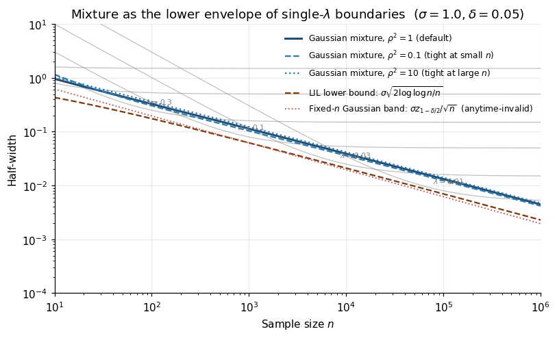
Three things to read off. (i) The boundary scales as for large — a factor over the fixed- Hoeffding bound. (ii) The parameter is a bias–variance dial: large tight at small , small tight at large . Optimal for design horizon gives the tightest CS near . (iii) The boundary (4.4) is the lower envelope of all single- boundaries (by Jensen on the log in (4.1)) — for every , the mixture is at worst a small constant factor wider than the best single- choice for that .
4.4 Why mixtures almost match the LIL rate
The Gaussian mixture boundary is ; the LIL lower bound is . The ratio is — at , . Closing the gap requires heavier-tailed mixing densities:
- Stitched discretized mixtures (Howard et al. 2020, §4). Discretize a geometric grid of design horizons , take a separate single- boundary tight at each , and union-bound them with weights . Matches LIL with explicit constants. No closed form.
- Predictable-mixture / betting boundaries (Waudby-Smith and Ramdas 2024). Replace fixed with a data-dependent (predictable) sequence . Formally tighter than any fixed-prior mixture and matches the LIL rate. Developed in §6.
For practical horizons (), the Gaussian-mixture’s – widening over LIL is a modest price for the closed-form expression (4.3), and most A/B-testing platforms ship it as default. The formal LIL lower bound is in §13.3.
5. The Howard–Ramdas–McAuliffe–Sekhon boundary atlas
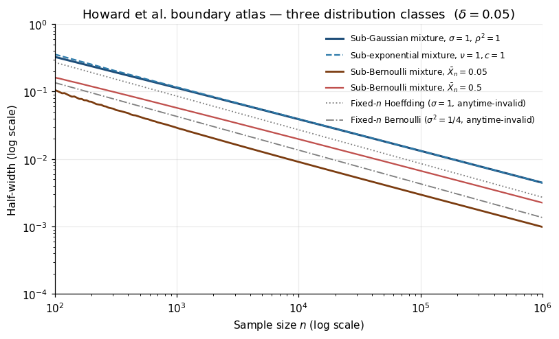
§§2–4 built one confidence sequence — the sub-Gaussian Robbins mixture. The systematic observation of Howard, Ramdas, McAuliffe, and Sekhon (2020), the paper that systematized the modern field, is that every fixed- Chernoff bound has a time-uniform analogue. This section catalogues the three boundary classes that cover essentially every applied use of AVI: sub-Gaussian, sub-exponential, sub-Bernoulli.
5.1 The Wald–Doob exponential supermartingale
For i.i.d. with , define the centered CGF . The Wald–Doob exponential martingale is
Lemma 5.1 (Sub-class supermartingale).
Let upper-bound on an interval : . Then is a nonnegative supermartingale with for every .
Proof.
Nonnegativity is immediate. One-step ratio:
since .
∎Recipe. Pick a distribution class → choose → build → mix over → apply Ville → invert.
5.2 Sub-Gaussian boundaries
For sub-Gaussian variance proxy , for all . The single- boundary is a straight line in the plane with intercept and slope . The Robbins mixture (4.4) sits along the lower envelope of all these lines, at the cost of a excess over LIL. This is the baseline anytime-valid boundary.
5.3 Sub-exponential boundaries via Bernstein tilting
Sub-Gaussian excludes Poisson, , exponential. The next-most-permissive class is sub-exponential.
Definition 5.2 (Sub-exponential).
A random variable with mean is sub-exponential with parameters if
is the variance scale, controls exponential-tail behavior. Setting recovers sub-Gaussian.
Examples. Centered Poisson is sub-exponential with ; centered has ; centered Exponential(1) has .
The time-uniform Bennett-mixture CS has asymptotic form
For , the tail correction is negligible.
Example 5 (Poisson CS).
: . — the anytime-valid analogue of the Wald rate-ratio CI.
5.4 Sub-Bernoulli boundaries via the binary KL function
For bounded with mean , the Bernoulli MGF gives a tighter bound than worst-case sub-Gaussian .
Lemma 5.3 (Bernoulli MGF bound).
If with ,
with equality iff is Bernoulli.
Proof.
is convex. For , . Take expectation.
∎Taking logs: . The fixed- Chernoff bound under this MGF is where is the binary KL function. This is tighter than sub-Gaussian Hoeffding (which uses ); the asymmetry of binary KL near or captures the rare-event regime correctly.
The Wald–Doob supermartingale is , a martingale under Bernoulli. Mixing in the Bayesian-updated -parametrization with gives the Beta-binomial marginal likelihood ratio
The CS is the set of where — implicit, computed by bisection.
Example 6 (A/B test for conversion lift).
: sub-Gaussian Hoeffding gives (relative half-width 86%, useless). Sub-Bernoulli mixture CS gives (relative half-width 36%). The sub-Bernoulli adapts to via the asymmetric KL.
5.5 Numerical comparison with fixed- Hoeffding
Setup: , , . Fixed- Hoeffding: .
| Fixed- Hoeffding | Sub-Gaussian mix (4.4) | Ratio | Sub-Bern. mix @ | Ratio | |
|---|---|---|---|---|---|
The sub-Gaussian mixture is – wider than fixed- Hoeffding — the cost of anytime-validity. Sample-size cost is –. The sub-Bernoulli at low conversion rates is tighter than fixed- Hoeffding via the binary KL.
Aggressive stopping rule; B = 1500 replicates per class.
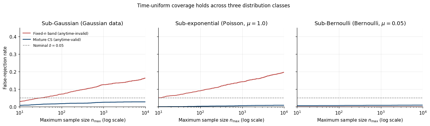
Practitioner verdict. For bounded data, sub-Bernoulli by default. For sub-Gaussian data, Robbins mixture (4.4). For Poisson//exponential, Bennett mixture (5.9) with correction (negligible for ).
6. Empirical-Bernstein and predictable mixtures — the betting reformulation
§5’s atlas got us most of the way, but two limitations linger. First, the sub-Gaussian and sub-exponential boundaries use worst-case variance proxies; for low-variance data the boundary is loose by a substantial factor (e.g., for Bernoulli at ). Second, the closed-form Gaussian-mixture has a residual excess over LIL. The reformulation that fixes both is due to Waudby-Smith and Ramdas (2024), built on game-theoretic probability (Vovk, Shafer) and Kelly’s (1956) information-theoretic gambling.
6.1 Variance adaptation as wealth accumulation
For small , expand . Replace the worst-case correction with the empirical per-step , giving the product form:
A cumulative product, not an exponential of a sum — the wealth process of a gambler betting fraction at each round.
Definition 6.1 (Betting wealth, fixed λ).
For i.i.d. with under and , the betting wealth process is (6.1) with .
Lemma 6.2 (Fixed-bet wealth is a martingale under H_0).
Under Definition 6.1, is a nonnegative martingale with .
Proof.
Nonnegativity is from the constraint. One-step ratio:
Multiplying by and induction with gives the claim.
∎Variance adaptation as the headline win. For Bernoulli at : , but worst-case sub-Gaussian . The boundary based on is wider than what the actual data warrant. The betting wealth recovers that factor automatically by using the actual deviations .
6.2 Predictable processes and Kelly bets
The fixed- wealth (6.1) is already a martingale. Lemma 6.2 has more to offer: the property survives when is a predictable process.
Definition 6.3 (Predictable bet schedule).
A sequence is predictable if is -measurable for each . The predictable-bet wealth process is
Theorem 6.4 (Predictable wealth is a martingale under H_0).
With predictable and positivity-preserving, is a nonnegative martingale with .
Proof.
By predictability, is -measurable, so
∎
Predictability preserves the unbiasedness while letting be learned from prior observations.
Definition 6.5 (Kelly-optimal bet).
Under alternative with , the Kelly-optimal bet is
Two reasons: (i) expected detection time is approximately where , so maximizing minimizes detection time; (ii) by the LLN, almost surely.
Closed-form Kelly for small bets. First-order expansion gives the approximation
For Bernoulli the exact closed form is — see (9.7) in §9.3. The two agree to leading order in .
Empirical Kelly. Plug in the running estimates:
Each depends only on , hence predictable.
6.3 Waudby-Smith–Ramdas (2024) bounded-variable boundaries
Waudby-Smith and Ramdas (2024) systematized the betting approach for bounded . The PrPl-EB schedule (predictable plug-in, empirical Bernstein):
Theorem 6.6 (Empirical-Bernstein CS (Waudby-Smith and Ramdas 2024, Theorem 2)).
For i.i.d. bounded on with mean and variance , the PrPl-EB CS satisfies , and asymptotically
LIL match with the true variance , not the worst-case bound. This closes both the LIL gap (cf. §13.3) and the variance-adaptation gap at once.
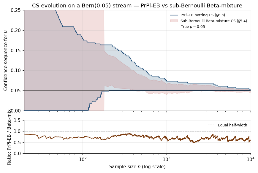
Example 7 (PrPl-EB beats Beta-mixture for low μ).
At : PrPl-EB half-width ; sub-Bernoulli Beta-mixture . A reduction.
6.4 Practical numerical computation
Log-space computation. Always store , never directly. Overflow at for GRO bets on well-separated data.
CS endpoint computation via bisection. is unimodal in ; CS endpoints are roots of via bisection. Tolerance suffices.
Clipping for positivity. for . Standard .
Forward-pointing. The betting wealth is the prototype of what §8 calls an e-process. The Kelly criterion is the prototype of §9’s growth-rate optimality. §10’s merging operations combine wealth processes from independent experiments.
8. e-values and e-processes
We’ve spent six sections building one object — a nonnegative (super)martingale with unit initial expectation that we plug into Ville — under three different names. In §3 it was Wald’s likelihood ratio. In §§4–5 it was a Robbins mixture. In §6 it was Waudby-Smith–Ramdas’s betting wealth. The structural identity, since Vovk (1993) and Vovk and Wang (2021), is the e-value / e-process. This section formalizes the concept, states the duality between e-processes and anytime-valid tests, catalogues the e-processes already built, and develops the bridge to p-values.
8.1 Definition — E[E] ≤ 1
Definition 8.1 (e-value).
Let specify . A nonnegative random variable is an e-value for if
“e” for “expectation-bounded” or “evidence.” The budget "" is the catch: under the null, can’t on average exceed . Spending that budget on the tail — making small — is the test design problem.
Lemma 8.2 (Markov's inequality gives the e-test).
For an e-value and ,
Proof.
Markov applied to with : .
∎(8.2) is the single-shot level- test: reject when .
Definition 8.3 (e-process).
A sequence of e-values adapted to is an e-process for if it is a nonnegative supermartingale under with .
An e-process is a predictable strategy for spending the unit budget over time.
8.2 From e-value to anytime-valid test via Ville
Theorem 8.4 (Anytime-valid test from an e-process).
For an e-process and any and stopping time ,
Proof.
Set inclusion plus Ville (Theorem 2.3) at threshold using .
∎Theorem 8.5 (e-process / anytime-valid-test duality (informal)).
Every sequence of -valued anytime-valid tests at level arises from an e-process via for some e-process .
Precise statement and proof in Howard et al. (2020, §2.3) and Ramdas et al. (2023, Theorem 4.1). Anytime-valid testing IS e-process testing.
8.3 The likelihood ratio as the canonical e-process
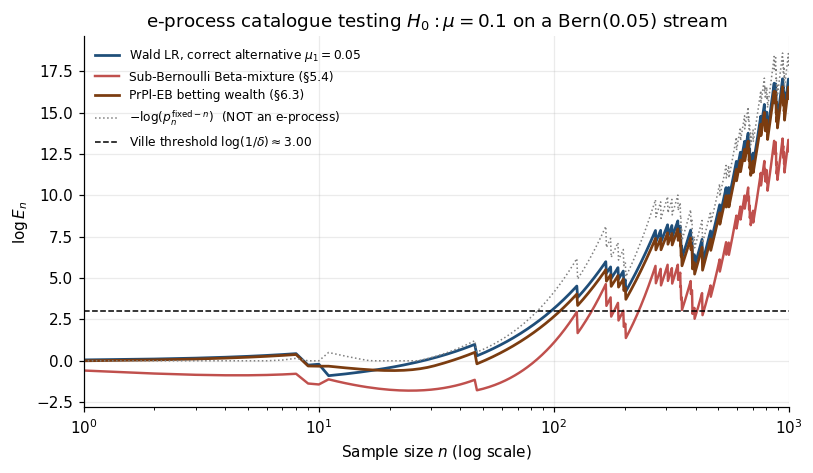
The constructions of §§3–6 are all e-processes:
- §3: Wald’s LR. by Lemma 3.1. ✓
- §§2, 4, 5: Wald–Doob supermartingales and mixtures. ✓ (sub-Gaussian, sub-exponential, sub-Bernoulli variants).
- §6: Betting wealth. ✓
The likelihood ratio is the canonical e-process; every other construction is a relaxation or generalization for the composite-alternative case.
Example 8 (Reading off the type-I error guarantee).
Sub-Bernoulli Beta-mixture e-process on conversion data: at , . By (8.4), the rejection rule “reject when ” has type-I error — for every stopping rule.
8.4 e-to-p calibration and the calibrator-of-calibrators
Definition 8.6 (p-value).
is a valid p-value for if for every .
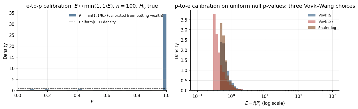
Lemma 8.7 (e-to-p calibration).
For an e-value , is a valid p-value.
Proof.
for , so by Lemma 8.2.
∎For an e-process, is a running anytime-valid p-value sequence.
The p-to-e direction is harder. The naive fails: for .
Definition 8.8 (p-to-e calibrator).
is a p-to-e calibrator if is an e-value whenever is a valid p-value.
Theorem 8.9 (Vovk and Wang 2021, calibrator characterization).
is a p-to-e calibrator iff is decreasing, upper semi-continuous, and . Admissible calibrators have and are generated by for concave with .
Proof in Vovk and Wang (2021, §2). Examples include the Vovk family for and the Shafer logarithmic .
Why the asymmetry. e-to-p is canonical (lossless); p-to-e is non-canonical (lossy). p-values are rank statements; e-values are magnitude statements. e→p collapses magnitude into rank; p→e tries to recover magnitude from rank (impossible without extra structure). Takeaway: start with an e-process and report e-values directly; convert to p-values for reader-friendliness only.
9. Growth-rate optimality, the Kelly connection, and universal e-processes
§8 named the e-process and showed every anytime-valid test is one. But it didn’t say which e-process is the right one. This section provides the optimality theory. The key concept is growth-rate optimality (GRO): the e-process that maximizes expected log-growth under the alternative is the fastest-detecting anytime-valid procedure. For simple-vs-simple, the GRO e-process is Wald’s likelihood ratio, and its growth rate equals the KL divergence — closing the loop from §3.4 to a sharp theorem. The same criterion has a 70-year-old gambling interpretation (Kelly 1956). For composite alternatives, universal e-processes match the alternative’s KL up to logarithmic regret, generalizing Cover’s (1991) universal portfolios.
9.1 GRO — definition and the optimization problem
Definition 9.1 (Growth rate of an e-process).
For e-process and alternative ,
For i.i.d. data and multiplicative-product e-processes , .
Definition 9.2 (Growth-rate-optimal e-process (Grünwald and Koolen 2022; Shafer 2021)).
Let denote the set of all e-processes for . The GRO e-process for testing against is
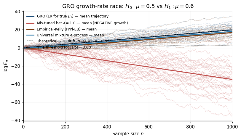
Why log-growth, not raw growth? has no upper bound (aggressive bets give arbitrary mean growth). But by LLN, almost surely under — maximizing log-growth corresponds to maximizing the typical detection rate.
9.2 KL divergence as the optimal growth rate
Theorem 9.3 (GRO theorem for simple-vs-simple).
For , with mutually absolutely continuous, is GRO with . For any other e-process , .
Proof.
Step 1: is an e-process by Lemma 3.1.
Step 2: .
Step 3: For any e-process with , by Jensen (concavity of ):
The Radon–Nikodym derivative , so
Hence .
∎The same KL divergence governs fixed- Chernoff exponents (Neyman–Pearson, Stein’s lemma) and anytime-valid growth rates. The LR achieves both simultaneously.
Operational consequence. Expected stopping time of the GRO rejection rule:
This is the §3.2 SPRT efficiency calculation reinterpreted: the SPRT achieves the minimum stopping time because the LR is GRO. The Wald–Wolfowitz theorem (§3.3) is the same statement in classical-statistics language.
9.3 The betting interpretation
Kelly’s setup: a gambler with bankroll . At each round, outcomes with true probabilities and “fair” odds . Per-round log-growth at portfolio :
Maximizing over gives the Kelly bet — bet proportional to true probability.
Theorem 9.4 (Kelly 1956 — optimal gambling growth rate).
The Kelly bet achieves , the maximum expected log-growth.
The bridge. Theorem 9.4 and Theorem 9.3 say the same thing in different languages:
| Anytime-valid testing | Kelly gambling |
|---|---|
| Null | Bookmaker’s odds |
| Alternative | True probabilities |
| e-process with | Wealth process at fair odds |
| GRO e-process (LR) | Kelly bet () |
An e-process for is the wealth of a gambler placing fair bets at the odds implied by . This is the test by betting perspective of Shafer (2021) and the game-theoretic probability program of Shafer and Vovk (2019).
Empirical Kelly and the §6 betting wealth. For Bernoulli with null and unknown alternative, the exact Kelly bet (solving (9.2) for simple Bernoulli alternatives) is
with Kelly growth rate equal to the binary KL: . The empirical Kelly substitutes for — the predictable plug-in rule (6.5).
Example 9 (Bernoulli Kelly explicit).
: . Kelly rate . Expected detection time at : — matches §6 simulation.
A note on over-betting. The §9 simulation also evaluates (over-aggressive). For Bernoulli vs Bernoulli, gives expected log-growth — negative. Over-betting beyond Kelly’s optimum is strictly worse than not betting at all; this is the Kelly criterion’s most counterintuitive consequence: under-aggressive () only loses efficiency, but over-aggressive ( for symmetric Bernoulli) actually loses wealth.
9.4 Universal portfolios as universal e-processes
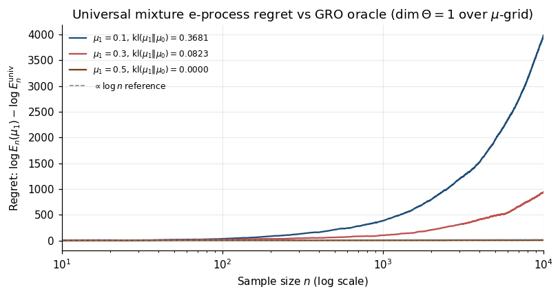
The GRO theorem assumes a known alternative. In practice the alternative is composite; no single e-process can be GRO simultaneously for every .
Cover (1991) addressed this for portfolio selection. Cover’s universal portfolio achieves uniformly over all return sequences.
Translation to e-processes. Replace “stock returns” with “per-observation betting wealth ratios.” The construction becomes the Robbins-mixture e-process
Theorem 9.5 (Universal e-process (mixture form, informal)).
Under regularity conditions on , for any ,
Proof via Laplace approximation. Full development in Cover (1991), Barron and Hengartner (1998), Grünwald and Koolen (2022, §4).
Structural significance. Universal e-processes generalize universal source codes (Cover and Thomas 2006, ch. 13) from information theory. A universal source code achieves the entropy rate of any source in a class up to overhead per symbol; a universal e-process achieves the KL-growth rate of any alternative in a class up to overhead per observation. The MDL principle (Grünwald 2007) recognizes both as instances of one principle.
For the practitioner: universal e-processes give honest, anytime-valid inference for composite alternatives without requiring parametric likelihood specification or prior. The cost is regret — at and , extra observations on top of the GRO oracle’s expected .
10. Merging e-values
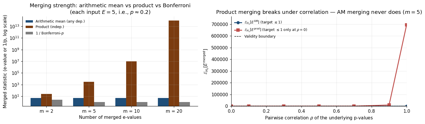
A single test rarely lives in isolation. A modern A/B-testing platform runs hundreds of concurrent experiments; a meta-analyst pools evidence from a dozen studies; a bandit tracks rewards across arms. The classical answer is Bonferroni on p-values — honest but punitively conservative. E-values handle the combination dramatically better. Arithmetic-mean merging is valid under arbitrary dependence. Product merging under independence is dramatically tighter than even the most efficient p-value combiner. Vovk and Wang (2021) prove that arithmetic mean is the dominant symmetric merger under arbitrary dependence.
10.1 Arithmetic mean — robust under arbitrary dependence
Theorem 10.1 (Arithmetic-mean merger).
Let be e-values for with arbitrary joint distribution. The arithmetic mean is an e-value for .
Proof.
Nonnegativity is immediate. By linearity:
Linearity does not require independence.
∎The dependence structure can be anything and the arithmetic mean remains valid. Compare with p-values: the smallest p-value is not generally a valid p-value (Bonferroni loses a factor of ); the arithmetic mean of e-values loses nothing.
Extending to e-processes. If are e-processes with arbitrary cross-dependence, is itself an e-process (Theorem 10.1 + Theorem 4.1). Anytime-valid meta-analysis with no dependence assumption.
Example 10 (A/B testing across user segments).
segment-level e-processes testing per-segment treatment effect. We want global anytime-valid test of “no effect in any segment.” Segments may be correlated (shared platform-level confounders). Arithmetic-mean process is anytime-valid for the global null — no Bonferroni, no covariance estimation.
10.2 Geometric mean and product — independence required
Theorem 10.2 (Product merger under independence).
Let be jointly independent e-values for . The product is an e-value.
Proof.
By independence, .
∎The product can be exponentially larger than the arithmetic mean. for : , . Independent observations let us multiply our beliefs.
Geometric mean is dominated. pointwise (AM–GM); no reason to prefer it.
10.3 The Vovk–Wang (2021) merging-function characterization
Definition 10.3 (E-merging function).
A symmetric is an e-merging function under arbitrary dependence if is an e-value whenever each is, regardless of joint distribution.
Theorem 10.4 (Vovk and Wang 2021, Proposition 3.1).
Every symmetric e-merging function under arbitrary dependence is dominated pointwise by the arithmetic mean:
Proof in Vovk and Wang (2021, §3). The arithmetic mean is the unique (up to dominated alternatives) optimal symmetric e-merging function under arbitrary dependence.
Weighted means with are also valid mergers; encode prior beliefs about study quality.
Contrast with p-value merging. The unique symmetric p-merging function under arbitrary dependence is Bonferroni. There is no p-value analogue of the arithmetic-mean merger that improves linearly in without independence assumptions. The asymmetry: e-value’s is a linear constraint (Jensen-friendly); p-value’s is a quantile constraint (adds up under worst-case dependence — Bonferroni).
10.4 When you should not Bonferroni
Bonferroni is right when (i) tests are fixed-sample, (ii) is small, (iii) external constraint demands p-values. For every other multiple-testing setting, e-value merging is dramatically better. Four headline cases:
Sequential multiple testing. Platform runs concurrent A/B tests, peeking at each. Bonferroni on fixed- p-values gives per-test — compounds with sequential widening. E-value alternative: maintain anytime-valid per test, merge via . Global type-I at is by Ville. No Bonferroni.
Online FDR control. LORD/SAFFRON for p-values; e-LOND/e-LORD (Wang and Ramdas 2022) for e-values. The e-value versions use the wealth-process structure directly; strictly more powerful under independence.
Meta-analysis with unknown correlation. Random-effects models assume distributional structure; e-value AM merger is assumption-free.
Bandit / off-policy evaluation. Adaptive sampling breaks standard CIs. Per-arm e-process CSs (Karampatziakis–Mineiro–Ramdas 2021) merged via AM give a global anytime-valid CS for the policy value.
Unifying message. e-values let you merge across studies, segments, and time without paying the Bonferroni penalty.
11. ML applications — A/B testing, bandits, and adaptive data
This section closes the loop to practice. Every modern A/B-testing platform ships an anytime-valid CS as the default stopping criterion. Every contextual-bandit deployment that needs honest evaluation uses off-policy e-processes. The shift, between roughly 2017 and 2022, replaced the fixed-horizon Wald test that had been standard for two decades.
11.1 Modern experimentation platforms
The commercial A/B-testing market has standardized on anytime-valid methodology:
| Platform | Anytime-valid construction | Reference |
|---|---|---|
| Eppo | Gaussian-mixture CS + PrPl-EB for binary | Eppo methodology docs |
| Statsig | Sequential probability ratio test + mixture CS | Howard et al. (2020) |
| Optimizely “Stats Engine” | Mixture sequential probability ratio test (mSPRT) | Johari, Pekelis, Walsh (2015); Johari et al. (2017) KDD |
| Microsoft EXP | Sequential tests + mixture CS, internal use | Deng et al. (2016) DSAA |
| LinkedIn Experimentation | mSPRT for binary, Gaussian-mixture for continuous | Xu et al. (2015) KDD |
| Netflix | Anytime-valid linear models / sequential causal | Lindon, Ham, Tingley, Bojinov (2022) |
| VWO | Bayesian sequential testing (posterior-CS) | VWO methodology docs |
All seven platforms ran fixed-horizon -tests as default in 2015. By 2022 all seven had transitioned to some form of anytime-valid reporting. The shift was driven by practitioner demand: analysts want to look at the dashboard daily and make calls in real time, and the fixed-horizon framework offered no honest way to do that. Johari, Koomen, Pekelis, and Walsh (2017) “Peeking at A/B tests” made the §1 peeking failure explicit.
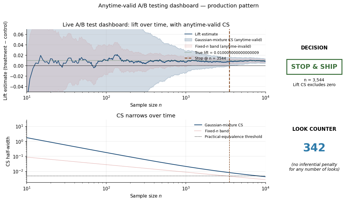
11.2 Anytime-valid stopping criteria in practice
The operational pattern across platforms looks essentially identical.
Step 1 — Specify the metric and inferential target. Lift in revenue per user, conversion rate, retention, etc. (two-sided) or (one-sided).
Step 2 — Choose the CS construction. Continuous: sub-Gaussian Robbins mixture (4.4). Counts: sub-exponential Bennett mixture (5.9). Binary: sub-Bernoulli Beta-mixture (5.14) for , PrPl-EB betting CS (6.6) for boundary means.
Step 3 — Pick the level and mixing parameter. . Mixing tuned for expected horizon .
Step 4 — Run and monitor. CS updates as observations stream in. Three actions: continue, stop-and-ship (CS excludes null favorably), stop-and-abandon (CS narrow enough to declare practical equivalence).
The crucial property: the stopping rule does not need to be pre-specified. Whether the analyst stops at or , the type-I error guarantee holds.
Quantifying the cost. §5.5 showed – sample-size cost vs fixed- at the same nominal width. Operationally: an experiment that “would have” reached power at with fixed-horizon typically needs with anytime-valid CS if run to the planned horizon. Savings come from not having to — strong effects detected at a fraction of . Platforms report 20–40% reduction in average experiment duration vs fixed-horizon baseline.
11.3 Off-policy confidence sequences for bandits
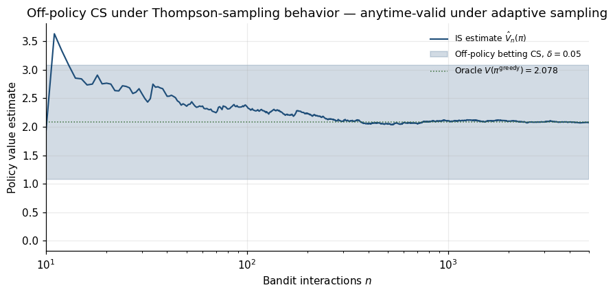
Modern recommendation systems use contextual bandits with adaptive sampling — action probabilities depend on history. Standard i.i.d. analysis breaks.
The standard OPE estimator:
Karampatziakis, Mineiro, and Ramdas (2021) constructed anytime-valid CSs for :
By Theorem 6.4 + Ville, this is anytime-valid. Works under arbitrary adaptive behavior policies — the behavior policy can depend on the entire history.
Example 11 (Continuous-monitoring contextual bandit).
News-recommendation system with 5-arm Thompson sampling bandit. Product team wants anytime-valid 95% CS for each arm’s expected CTR. Using (11.2) with importance weights from Thompson’s posterior, CS updates at each impression. After 100,000 impressions, CSs of width ≈ 0.02 around each arm — honest decisions about which arms to retire. The bandit’s exploration probabilities changing in real time does not invalidate the CSs.
11.4 Causal-effect-under-policy-shift extensions
Bibaut, Petersen, Vlassis, Dimakopoulou, and van der Laan (2021) “Sequential causal inference in a single world of connected units” handles time-evolving populations: treatments assigned over time (possibly adaptively), target causal estimand changes as population shifts, anytime-valid inference for the current estimand. Combines doubly-robust estimation (outcome models + propensity scores) with §6 betting-wealth machinery. Under standard rate conditions ( for nuisance), the CS is anytime-valid for time-varying causal estimands.
Three increasingly difficult scenarios: (i) static treatment + outcome drift; (ii) static treatment + covariate drift; (iii) adaptive treatment policy. The third subsumes the bandit case and extends to confounders, IVs, and Athey–Imbens-style econometric extensions.
11.5 Common pitfalls
Pitfall 1 — Treating fixed- CIs as “almost” anytime-valid. Wrap fixed- Gaussian band in “stop after ” rule. The §1.2 simulation: , , empirical false-rejection at . Fixed- band is not anytime-valid for any .
Pitfall 2 — Miscalibrating the mixing prior. gives tightest CS near . Fix: tune to expected stopping time, or use PrPl-EB (parameter-free, self-tunes).
Pitfall 3 — Confusing CS coverage with sample-mean accuracy. CS is an interval estimate for the population parameter — not a prediction interval for the sample mean’s future trajectory.
Pitfall 4 — Neglecting multi-test merging from §10. concurrent A/B tests at per-test → family-wise error if naively interpreted. Right fix: arithmetic-mean merging (Theorem 10.1) for global test; e-LOND/e-LORD for FDR control.
Pitfall 5 — Reporting CS at horizon without context. CS at single is wider than fixed- CI by . Report CS width with operational context — the CS bought the right to stop at any , including much earlier if evidence accumulated quickly.
Unifying message: anytime-validity is a property of the inference procedure, not a label slapped on a fixed- statistic.
12. Computational notes
Four implementation concerns recurred across §§3–11. Collected here as a reference.
12.1 Numerical stability at large
Always compute e-processes in log-space. Betting wealth overflows Float64 () at on well-separated data. Universal fix: log_K_n = np.cumsum(np.log1p(lambdas * (X - mu))) — stable to .
Log-sum-exp for mixture e-processes. : shift by before exponentiating. scipy.special.logsumexp.
Cumulative-max for “ever-crossed” computations. np.maximum.accumulate(E_traj, axis=1) for the running supremum in vectorized time.
Positivity-preserving clip. for . Standard .
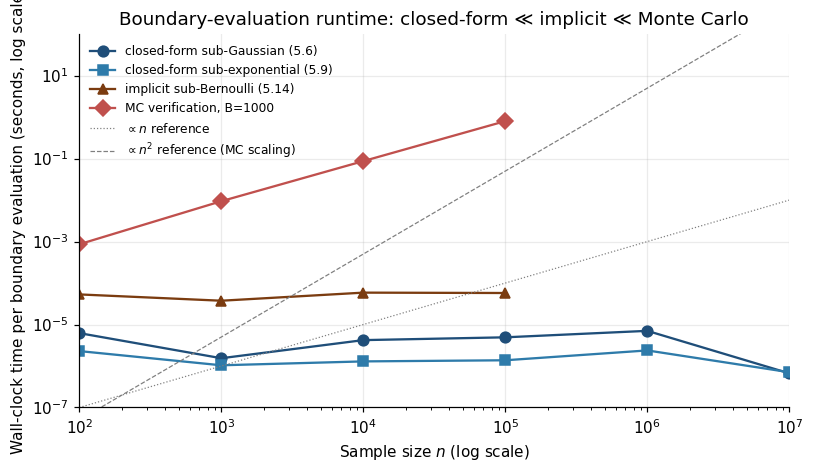
12.2 Closed-form vs Monte Carlo boundary evaluation
Closed-form (sub-Gaussian (4.4), sub-exponential (5.9)): pre-compute boundary as function of . per . Right call for production A/B-testing.
Implicit + bisection (sub-Bernoulli (5.14), PrPl-EB (6.6)): roots of via bisection. per .
Streaming update pattern. Maintain fixed grid of candidate values, update each in per new observation. Per-observation cost .
12.3 Special-function inversions
scipy.special.betalnfor sub-Bernoulli Beta-mixture (5.14). Overflow-safe.scipy.special.lambertw(z, k=0).realfor sub-exponential boundary equations .- Inverse binary KL via
brentqon . scipy.stats.norm.ppf(1 - \delta/2)for fixed- Gaussian quantile reference.
12.4 Reproducibility
Use np.random.default_rng(seed), not np.random.seed(). Per-experiment RNG with explicit state.
Seed-locked verification. Print MC summaries; numbers should reproduce exactly on fresh kernel run.
Numerical-determinism caveats. Float arithmetic is bit-deterministic; parallel BLAS reductions may reorder summations ( variation in -term sums). Below MC noise floor for these simulations.
13. Connections and limits
We close by situating AVI in the broader formalML landscape and surveying what the framework can’t yet do.
13.1 AVI vs PAC-Bayes — the same Ville step, two applications
The most striking structural identity in this topic: AVI and PAC-Bayes Bounds use the same supermartingale + Ville machinery for different applications.
PAC-Bayes: with prior and posterior , the bound
via Donsker–Varadhan + Markov on an exponential PAC-Bayes supermartingale.
AVI: with null and e-process , the bound via Markov on Wald–Doob’s supermartingale + GRO with rate .
The two differ in application: PAC-Bayes is generalization (loss of a randomized predictor); AVI is testing (type-I error of a sequential test). The mathematical engine — Markov + supermartingale + KL change-of-measure via Donsker–Varadhan — is identical. The Donsker–Varadhan inequality is the central tool in both proofs:
A reader who has done pac-bayes-bounds and this topic has met the same theorem twice. That unification is the central contribution of the game-theoretic probability program (Shafer and Vovk 2019).
13.2 AVI vs selective inference — different conditioning events
The structural cousin one track over is Selective Inference (T6). Both address the same family of practitioner failures with different conditioning.
Selective inference handles model-selection-induced peeking. After lasso, condition on the polyhedral selection event . Truncated-Gaussian pivot (Lee, Sun, Sun, Taylor 2016).
Always-valid inference handles time-induced peeking. After A/B test, condition on stopping-time event . Robbins mixture (§4) and PrPl-EB betting (§6).
| Selective inference | Always-valid inference |
|---|---|
| Selection event Ay ≤ b (polyhedral) | Stopping-time event τ ≤ n (data-adaptive) |
| Truncated-Gaussian pivot | Time-uniform Ville bound |
| Conditional CI given selection | Anytime-valid CS over stopping rules |
| Power loss as price of post-selection honesty | Sample-size cost as price of optional-stopping honesty |
Complementary, not competing. A platform that runs an experiment, performs feature selection, and reports a CI should use both.
13.3 The LIL lower bound and the constant gap
The §1.3 preview promised LIL as the asymptotic floor. The formal Hartman–Wintner (1941) statement:
Stopping-time lifting gives: no -confidence sequence can have half-width smaller than for all simultaneously. Proof via the LIL almost-sure envelope crossing any narrower-than-LIL band at some random stopping time.
Asymptotic picture across the three regimes:
- Fixed- Hoeffding (anytime-invalid): — pure .
- Gaussian-mixture CS (4.4): — extra .
- PrPl-EB betting CS (6.6, LIL-matching): — extra .
- LIL lower bound: (the hard floor).
At , ; unavoidable cost over fixed- is in width, in sample size. PrPl-EB hits this exactly; Gaussian mixture pays an extra at (total width, sample size). PrPl-EB is conjectured to be constant-optimal (Waudby-Smith and Ramdas 2024); formal proof open.
13.4 Composite nulls, nuisance parameters, and the frontier
The framework as developed handles simple and parametric-composite alternatives elegantly. Active frontier:
Composite nulls. requires . Grünwald, de Heide, Koolen (2024) “Safe testing” provides the framework. Larsson, Ramdas, Ruf (2024) give explicit constructions via online learning.
Nuisance parameters. Doubly-robust estimators + betting machinery: Bibaut et al. (2021) for causal nuisance.
Continuous-time AVI. Discrete- replaced by càdlàg supermartingales. Applications: high-frequency financial monitoring, physiological signal analysis.
Distribution-free / adversarial AVI. Cutkosky and Mhammedi (2024) — anytime-valid bounds under no distributional assumption, only an “online learning expert” structure.
Bayesian–frequentist hybrids. Variational posterior calibration via e-values: use Bayesian prediction, get frequentist coverage.
Multiple testing under arbitrary dependence. Wang and Ramdas (2022) e-LOND and e-LORD — online FDR procedures using e-process arithmetic; strictly more powerful than p-value-based equivalents.
13.5 Forward-pointers and the close
T6 Causal Inference Methods — doubly-robust + betting machinery (Bibaut et al. 2021) gives anytime-valid CIs for causal estimands under adaptive treatment.
T5 Bayesian Inference — §4.2 Bayes–frequentist correspondence — Robbins mixtures are Bayesian marginal likelihoods, interpreted frequentistically via Ville. Safe testing formalizes this duality.
T5 Variational Inference — e-value calibration of variational posteriors (Grünwald frontier).
T5 Sequential Monte Carlo — SMC importance-sampling weights have anytime-valid extensions via e-processes.
Closing. The AVI framework is the answer to the §1.1 question: how do we make honest inference under peeking? The classical fixed-horizon framework gives no answer — the §1.2 simulation showed false-rejection climbing to under peeking. AVI replaces the fixed-horizon assumption with anytime-validity, at the modest cost of a – sample-size widening. For modern data analysis — sequential A/B testing, multi-armed bandits, adaptive clinical trials, online causal inference, real-time monitoring of any kind — AVI is the right framework, and the e-process is the right primitive.
The conceptual scaffolding is small enough to hold in one’s head. A nonnegative supermartingale with unit initial expectation, run through Ville’s inequality. That single object — built as a Wald likelihood ratio, a Robbins mixture, a sub-class Wald–Doob supermartingale, or a Waudby-Smith–Ramdas betting wealth — handles every anytime-valid construction. The frameworks that look distinct (PAC-Bayes, selective inference, online FDR, off-policy evaluation, safe testing) use the same machinery with different problem-specific decorations.
What the practitioner gets is the operational right to peek. Dashboard checked at any cadence, experiment stopped at any sample size, decisions made based on current CS endpoints — all without inflating type-I error. The cost is the planned sample size at any single horizon, paid in exchange for the ability to stop early when evidence is overwhelming, which on average more than compensates. The platforms in §11.1 have all made this trade, and the §1 peeking analyst is no longer a problem to solve but a user whose intuitive workflow the framework was designed to support.
The mathematical machinery has been with us since Wald (1945) and Robbins (1970). What changed in the 2020s is the recognition — across academia (Howard et al. 2020, Waudby-Smith and Ramdas 2024) and industry (Optimizely, Eppo, Statsig, et al.) — that anytime-validity is the right default for modern data analysis, and that the supermartingale + Ville machinery is the right tool for delivering it. This topic was written from inside that recognition.
Connections
- AVI lifts every fixed-n Chernoff bound to a time-uniform analogue via Ville's inequality on the corresponding Wald–Doob supermartingale (§2.4). The sub-Gaussian, sub-exponential, and sub-Bernoulli boundary atlas of §5 IS the time-uniform extension of the Chernoff machinery developed there. concentration-inequalities
- Both topics use the same supermartingale + Ville + Donsker–Varadhan machinery for different applications: PAC-Bayes for generalization of randomized predictors, AVI for type-I error of sequential tests. The §13.1 structural identity makes this explicit — a reader who has done both has met the same theorem twice. pac-bayes-bounds
- The growth-rate-optimal (GRO) e-process for testing H_0: f_0 vs H_1: f_1 has expected log-growth equal to KL(f_1 || f_0). Theorem 9.3 identifies KL as the Cramér rate function in fixed-n large deviations AND the Kelly-optimal log-growth rate in anytime-valid testing — the same divergence governs both. kl-divergence
- Structural cousin one track over: both address post-hoc inference failures with different conditioning. Selective inference conditions on a polyhedral selection event Ay ≤ b; AVI conditions on stopping-time events τ ≤ n. The §13.2 comparison table makes the complementarity explicit. selective-inference
- The supermartingale framework (filtrations, adapted processes, Doob's optional-stopping theorem, Ville's inequality) is the measure-theoretic substrate. Every confidence-sequence construction in this topic instantiates the same template — choose a Wald–Doob supermartingale, mix it, apply Ville. measure-theoretic-probability
References & Further Reading
- paper On the Law of the Iterated Logarithm — Hartman & Wintner (1941) American Journal of Mathematics 63(1): 169–176. The almost-sure lim sup that makes peeking unavoidable.
- paper An invariance principle for the law of the iterated logarithm — Strassen (1964) Z. Wahrscheinlichkeitstheorie 3(3): 211–226. The sharp LIL constant.
- book Étude critique de la notion de collectif — Ville (1939) Gauthier-Villars, Paris. The original supermartingale-maximal inequality.
- paper Sequential Tests of Statistical Hypotheses — Wald (1945) Annals of Mathematical Statistics 16(2): 117–186. The SPRT, founding the field.
- paper Optimum Character of the Sequential Probability Ratio Test — Wald & Wolfowitz (1948) Annals of Mathematical Statistics 19(3): 326–339. The minimax-optimality theorem cited in §3.3.
- paper A New Interpretation of Information Rate — Kelly (1956) Bell System Technical Journal 35(4): 917–926. The log-optimal betting rule developed in §9.3.
- paper Confidence Sequences for Mean, Variance, and Median — Darling & Robbins (1967) PNAS 58(1): 66–68. First confidence-sequence constructions.
- paper Some Nonparametric Sequential Tests with Power One — Darling & Robbins (1968) PNAS 61(3): 804–809. Companion to the 1967 paper.
- paper Statistical Methods Related to the Law of the Iterated Logarithm — Robbins (1970) Annals of Mathematical Statistics 41(5): 1397–1409. The method-of-mixtures paper developed in §4.
- paper A Nonlinear Renewal Theory with Applications to Sequential Analysis II — Lai & Siegmund (1979) Annals of Statistics 7(1): 60–76. Refinements of Wald's identity and the SPRT efficiency theory.
- paper Universal Portfolios — Cover (1991) Mathematical Finance 1(1): 1–29. The construction lifted to §9.4 universal e-processes.
- paper A Logic of Probability, with Application to the Foundations of Statistics — Vovk (1993) JRSS B 55(2): 317–341. Game-theoretic probability and the early e-value concept.
- paper Time-uniform Chernoff bounds via nonnegative supermartingales — Howard, Ramdas, McAuliffe & Sekhon (2020) Probability Surveys 17: 257–317. The supermartingale-tooling paper underlying §§2 and 5; arXiv:1808.03204.
- paper Time-uniform, nonparametric, nonasymptotic confidence sequences — Howard, Ramdas, McAuliffe & Sekhon (2021) Annals of Statistics 49(2): 1055–1080. The confidence-sequence atlas cited in §§1.1, 4, 11.1; arXiv:1810.08240.
- paper Estimating means of bounded random variables by betting — Waudby-Smith & Ramdas (2024) JRSS B 86(1): 1–27. The PrPl-EB construction developed in §6.
- paper E-values: Calibration, combination, and applications — Vovk & Wang (2021) Annals of Statistics 49(3): 1736–1754. The calibrator and merging characterizations cited in §§8.4, 10.3.
- paper Safe testing — Grünwald, de Heide & Koolen (2024) JRSS B 86(5): 1091–1128 (with discussion). The safe-testing framework underlying composite-null AVI.
- paper Testing by betting: A strategy for statistical and scientific communication — Shafer (2021) JRSS A 184(2): 407–431. The test-by-betting perspective developed in §9.
- paper Log-optimal anytime-valid E-values — Grünwald & Koolen (2022) International Journal of Approximate Reasoning 141: 69–82. The GRO theorem and its log-optimal interpretation.
- paper Game-theoretic statistics and safe anytime-valid inference — Ramdas, Grünwald, Vovk & Shafer (2023) Statistical Science 38(4): 576–601. The standard survey reference for the field as of 2023.
- paper Always Valid Inference: Bringing Sequential Analysis to A/B Testing — Johari, Pekelis & Walsh (2015) arXiv. Deployed as Optimizely Stats Engine, Jan 2015.
- paper Peeking at A/B tests: Why it matters, and what to do about it — Johari, Koomen, Pekelis & Walsh (2017) Proc. 23rd ACM SIGKDD (KDD '17): 1517–1525. The §1 peeking pathology made explicit.
- paper Continuous Monitoring of A/B Tests without Pain: Optional Stopping in Bayesian Testing — Deng, Lu & Chen (2016) IEEE DSAA 2016. Microsoft EXP's deployment of sequential testing; arXiv:1602.05549.
- paper From Infrastructure to Culture: A/B Testing Challenges in Large Scale Social Networks — Xu, Chen, Fernandez, Sinno & Bhasin (2015) Proc. 21st ACM SIGKDD (KDD '15): 2227–2236. LinkedIn's experimentation platform paper.
- paper Anytime-Valid Linear Models and Regression Adjusted Causal Inference in Randomized Experiments — Lindon, Ham, Tingley & Bojinov (2022) Netflix's AVI methodology paper.
- paper Off-Policy Confidence Sequences — Karampatziakis, Mineiro & Ramdas (2021) Proc. 38th ICML, PMLR 139. The off-policy CS construction used in §11.3; arXiv:2102.09540.
- paper Sequential causal inference in a single world of connected units — Bibaut, Petersen, Vlassis, Dimakopoulou & van der Laan (2021) arXiv. The causal extension cited in §11.4.
- paper False discovery rate control with e-values — Wang & Ramdas (2022) JRSS B 84(3): 822–852. The e-LOND/e-LORD online-FDR procedures referenced in §§10.4, 11.5.
- paper Logarithmic Regret Algorithms for Online Convex Optimization — Hazan, Agarwal & Kale (2007) Machine Learning 69(2–3): 169–192. The Online Newton Step underlying AGRAPA.
- paper The numeraire e-variable and reverse information projection — Larsson, Ramdas & Ruf (2024) arXiv. Composite-null e-process constructions referenced in §13.4.
- paper Fully Unconstrained Online Learning — Cutkosky & Mhammedi (2024) NeurIPS 2024. The distribution-free / adversarial AVI frontier of §13.4.
- paper Exact post-selection inference, with application to the lasso — Lee, Sun, Sun & Taylor (2016) Annals of Statistics 44(3): 907–927. The selective-inference precedent compared against in §13.2.
- book Testing Statistical Hypotheses, 3rd ed. — Lehmann & Romano (2005) Springer Texts in Statistics. Ch. 4 develops the Wald–Wolfowitz minimax-optimality result.
- book Sequential Analysis: Tests and Confidence Intervals — Siegmund (1985) Springer Series in Statistics. Ch. II covers the SPRT in detail.
- book Probability with Martingales — Williams (1991) Cambridge UP. The standard textbook for martingale convergence and the optional-stopping theorem.
- book Game-Theoretic Foundations for Probability and Finance — Shafer & Vovk (2019) Wiley. The game-theoretic probability program underlying §§9 and 13.
- book High-Dimensional Statistics: A Non-Asymptotic Viewpoint — Wainwright (2019) Cambridge UP. Concentration-inequality machinery the fixed-n half of every result in §5 reduces to.
- book Elements of Information Theory, 2nd ed. — Cover & Thomas (2006) Wiley-Interscience. Ch. 13 (Universal Source Coding) is the information-theoretic side of the §9.4 universality argument.
- book The Minimum Description Length Principle — Grünwald (2007) MIT Press. MDL as the information-theoretic principle behind universal e-processes.