Selective Inference

1. Motivation

Most of statistical theory implicitly assumes the hypothesis was chosen before the data arrived. We pick a coefficient to test, we pick a model to fit, we pick an estimand to report — and then we look at the sample. The neat duality between point estimates, confidence intervals, and p-values that powers Stat 101 holds because that ordering holds: the hypothesis is fixed, the data is random, and the sampling distribution of the test statistic is a well-defined object.

Modern ML practice violates that ordering constantly. We fit a lasso on a thousand candidate features, look at the active set, and report confidence intervals on the selected coefficients. We screen a million SNPs against a phenotype, take the top hundred, and ask whether they’re real. We sit on top of an A/B-testing platform that runs ten thousand experiments a quarter and want to know how many of last quarter’s “winners” are actually wins. In each case the hypothesis was chosen by looking at the data, and the textbook guarantees — coverage, size, Type-I error, FWER, FDR — silently break.

Selective inference is the body of techniques that puts the guarantees back. It does so by being explicit about what was selected and how, and by re-deriving the sampling distribution conditional on the selection event itself. That single move — condition on what the selection procedure returned — turns out to support three otherwise quite different bodies of work: post-selection conditional inference (Lee, Sun, Sun & Taylor 2016) and debiased high-dimensional inference (Zhang & Zhang 2014; van de Geer, Bühlmann, Ritov & Dezeure 2014; Javanmard & Montanari 2014); finite-sample false-discovery control via knockoffs (Barber & Candès 2015; Candès, Fan, Janson & Lv 2018); and online FDR control via wealth processes (Foster & Stine 2008; Javanmard & Montanari 2018; Ramdas, Yang, Wainwright & Jordan 2018). This topic walks through all three.

1.1 The garden of forking p-values

The cleanest way to see the problem is to watch a familiar procedure fail on a familiar problem. Take a low-dimensional regression — $n = 100$ observations, $p = 20$ features, an identity design covariance, and a true coefficient vector $\beta^\star \in \mathbb{R}^{p}$ that is zero everywhere except on its first three entries, where it equals $1.5$. Standard regression theory says: fit OLS on all 20 features, get $\hat\beta$, and the 95% Wald interval $\hat\beta_j \pm 1.96 \cdot \mathrm{SE}(\hat\beta_j)$ covers $\beta_j^\star$ with probability $0.95$ for each $j$. That works. It works because the model — all twenty features — was fixed before the data arrived.

Now run the modern version. Fit the lasso with cross-validated $\lambda$, look at the active set $\hat S = \{j : \hat\beta_j^{\text{lasso}} \ne 0\}$, refit OLS on the selected features only, and report the Wald CIs from that fit. This is the workflow practitioners actually use — sklearn even ships it as a one-liner. The active set picks out, on average, around five to eight features per replicate: typically the three real signals plus several noise features that happened to correlate with $y$.

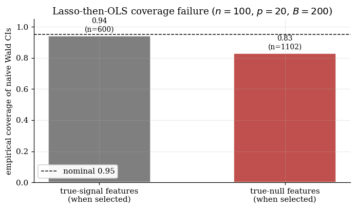
The CIs from this workflow look like normal CIs. They’re symmetric around the OLS-on-$\hat S$ point estimate, they have the usual $\pm 1.96$ structure, and they print out alongside a column labeled “95% CI” that nothing in the software flags as suspect. Their empirical coverage, however, isn’t $0.95$. Over $B = 200$ Monte Carlo replicates of this DGP, the signal-feature CIs cover their target with empirical probability $0.940$ — close to nominal, because the signal-to-noise ratio is high enough that the OLS-on-$\hat S$ estimate on a strong signal is approximately unbiased even after selection. But the null-feature CIs (features 4 through 20, when one of them sneaks into the active set on a particular replicate) cover their target — which is $\beta_j^\star = 0$ — with empirical probability $0.828$. The aggregate effect: a coverage rate that lands at $0.868$ on this toy.

The structural reason is selection bias on null features. The lasso selects feature $j$ precisely when $|X_j^\top (y - X_{-j}\hat\beta_{-j})|$ is large; the OLS-on-$\hat S$ coefficient on $j$ then inherits the conditional distribution of $X_j^\top y$ given that this quantity was large. For null features this conditional distribution is bimodal — concentrated away from zero on both sides — which is fundamentally different from the unimodal Gaussian the naive CI assumes. The CI is centered on a noisy estimate that’s never near zero conditional on selection, and on a non-trivial fraction of replicates it misses zero. Figure 1.1 quantifies the aggregate effect on the running toy.

This is the loss-of-coverage phenomenon that selective inference is designed to repair. The fix that conditional inference will deliver in §4 is structural: replace the unconditional sampling distribution of $\hat\beta_j$ with its conditional distribution given the selection event $\{\hat S = S\}$, and the resulting CI achieves nominal coverage. We’ll prove that in §4. For now, §1 just establishes the failure.

1.2 Three families of fixes

Selective inference is not a single procedure; it’s a programme. The procedures the topic covers cluster into three families, distinguished by what they condition on and what guarantee they deliver:

Conditional / post-selection inference (§§2–5). Condition on the realized selection event itself — for the lasso, the active-set and sign pattern $\{\hat S, \hat z\}$. The Lee–Sun–Sun–Taylor pivot delivers exactly nominal conditional coverage for any linear functional of $y$, including the partial OLS coefficients in the selected model. The debiased lasso of Zhang–Zhang / van de Geer et al. / Javanmard–Montanari delivers asymptotically nominal coverage in $p \gg n$ without conditioning, by computing a bias-corrected estimator whose CLT survives the selection bias.

Knockoff filters (§§7–9). Don’t condition; instead, construct fake “knockoff” features $\tilde X$ designed to be exchangeable with the real features under any null. Use this exchangeability to build a statistic per feature whose null distribution is sign-flip symmetric, then threshold on that distribution to control FDR. The finite-sample FDR guarantee holds at all $(n, p, q)$, with no asymptotic approximation.

Online FDR (§§10–11). When tests arrive in a stream — A/B platforms, continuous deployment, sequential genomics screens — neither BH nor conditional inference work directly because future tests aren’t yet visible. The α-investing / LORD / SAFFRON family solves this by tracking an α-wealth process: each test deducts from the wealth, each rejection deposits a payout, and a supermartingale argument bounds the running FDR by $\alpha$ at every stopping time.

The three families are not redundant. Each addresses a different practical bottleneck — small-but-non-trivial $p$ with a selection procedure (post-selection), $p \gg n$ with honest CIs needed (debiased), large-$p$ feature selection with finite-sample FDR (knockoffs), and streaming tests (online). The reader should leave §1 with one map and three distinct destinations; the §-by-§ exposition fills in each route.

1.3 What “selective inference” means precisely

The phrase admits several meanings in the literature; we’ll be specific. By “selective inference” we mean inference about a data-dependent estimand — a parameter, functional, or hypothesis that is itself a function of the sample. This is the unifying definition that covers all three families. In conditional post-selection inference, the estimand is the partial-OLS coefficient in the model selected by the lasso, and that model depends on $y$. In debiased high-dimensional inference, the estimand is a fixed coefficient, but the bias correction depends on a lasso fit. In the knockoff filter, the estimand is the set of features satisfying $X_j \not\perp Y \mid X_{-j}$, and the report (which features get flagged) depends on the data. In online FDR, the estimand is a sequence of null hypotheses, and the test schedule depends on the wealth process, which depends on the prior tests’ outcomes.

The parallel to semiparametric inference is structural and worth naming explicitly: semiparametrics asks for $\sqrt n$-valid inference about a low-dimensional functional in the presence of an infinite-dimensional nuisance estimated from data; selective inference asks for valid inference about a functional whose identity depends on data. Both topics live in the seam between “parameter is fixed, data is random” and “parameter and data are both random in a coupled way,” and both depend on a careful accounting of what randomness the inference is conditioning on. Where semiparametrics needs orthogonality of the influence function with respect to the nuisance score, selective inference needs an explicit description of the selection event whose probability the inference conditions on.

1.4 Roadmap and prerequisites

The topic proceeds in three arcs. §§2–5 cover post-selection and debiased inference: the LSST framework (§2), the polyhedral selection event for the lasso (§3), the truncated-Gaussian pivot (§4), and the debiased lasso (§5). §§6–9 cover knockoffs: the BH/Storey baseline (§6), the fixed-X knockoff filter and its supermartingale FDR proof (§7), the model-X generalization (§8), and the practical knockoff-construction linear algebra (§9). §§10–11 cover online FDR: the procedures (§10) and the wealth-process supermartingale proofs (§11). §12 lands the topic in ML applications, §13 collects computational notes, and §14 maps the connections to nearby topics and the limits of the framework.

The recommended prerequisites are high-dimensional regression for the lasso KKT conditions and debiased-lasso machinery, concentration inequalities for the martingale tail bounds that drive the online-FDR proofs, and ideally semiparametric inference for the conceptual frame on data-dependent estimands. From the sister site, formalStatistics’s Multiple Testing and False Discovery is the substrate selective inference generalizes — this topic discharges three forward-pointers from that page in a single ship.

2. The selection-event framework

§1 showed what goes wrong when we condition on the data twice — once implicitly through the selection procedure, once explicitly through the inference step — without accounting for the first conditioning. §2 sets up the framework that fixes it. The fix is conceptually simple: replace the unconditional sampling distribution of the test statistic with its distribution conditional on the selection event. The work of the rest of the topic is to make that conditional distribution computable.

This section sets the framework abstractly. §3 instantiates it on the lasso, §4 derives the truncated-Gaussian pivot that delivers the exact conditional CDF, §5 handles the high-dimensional case where exact conditioning is not available.

2.1 Hypotheses chosen by the data

Fix a sample space $\mathcal{Y}$ (think $\mathbb{R}^n$ for the regression setting). A selection procedure is a measurable map

$\mathcal{S}: \mathcal{Y} \to \mathcal{H},$

where $\mathcal{H}$ is a (countable, for simplicity) set of outcomes — model indices, active sets, threshold rules, anything we might run on the data before reporting a result. For the lasso at a fixed regularization $\lambda$, $\mathcal{S}(y) = (\hat S(y), \hat z(y))$ — the active set and sign pattern. For forward stepwise truncated at $K$ steps, $\mathcal{S}(y)$ is the ordered sequence of selected features. For the BH procedure at level $q$, $\mathcal{S}(y)$ is the set of rejected hypotheses.

Each outcome $s \in \mathcal{H}$ partitions the sample space into two pieces: the selection event

$E_s := \{y \in \mathcal{Y} : \mathcal{S}(y) = s\},$

and its complement. Conditioning on $E_s$ means restricting attention to the realizations that would have produced this particular selection outcome. The marginal sampling distribution of $Y$ — the one that classical inference uses — averages over all selection outcomes; the conditional sampling distribution $Y \mid \mathcal{S}(Y) = s$ averages only over realizations that hit $E_s$. The two coincide when $\mathcal{S}$ is constant (no selection — classical inference) and diverge otherwise. The size of the gap is what makes selective inference necessary.

A useful mental picture: $\mathcal{Y}$ is partitioned into selection cells $\{E_s\}_{s \in \mathcal{H}}$; the procedure stamps every observed realization with the label $s$ of whichever cell it lands in. Classical inference treats the whole sample space as the support of $Y$. Selective inference restricts to the cell we landed in and asks what the test statistic does inside that cell.

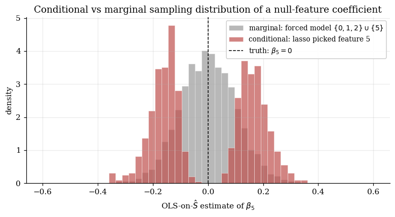
Numerical demonstration. On the §1 low-dim toy, fix the lasso regularization at a deterministic $\lambda$ (rather than CV — the conditional analysis needs a deterministic selection rule) and run $B = 4{,}000$ replicates. For each replicate, fit the lasso and record whether feature $j = 5$ (a true null) is selected. On the $\approx 20\%$ of replicates where feature 5 is in $\hat S$, compute the OLS-on-$\hat S$ estimate of its coefficient. Compare to a marginal reference: the OLS estimate of $\beta_5$ when the model is forced to include $\{0, 1, 2, 5\}$ from the start, regardless of what the lasso does.

The result, locked at notebook execution:

• Conditional sample (lasso selected feature 5): $n = 819$ out of 4000. Sample mean $-0.001$. Sample std $0.174$. Crucially, only 0.1% of conditional samples are in $(-0.05, +0.05)$; the distribution is bimodal, with $\approx 45.4\%$ of mass above $+0.10$ and $\approx 47.1\%$ below $-0.10$.

• Marginal sample (forced inclusion): $n = 4000$. Sample mean $+0.001$. Sample std $0.101$. Unimodal, peaked at zero.

The two distributions have similar means (both near zero, by symmetry) but qualitatively different shapes. The marginal distribution is the classical Gaussian $\mathcal{N}(0, \sigma^2/n)$ that Wald intervals are built around. The conditional distribution is bimodal — concentrated away from zero on both sides — because the selection event $\{j \in \hat S\}$ requires $|X_j^\top y|$ to have been large, which carves out the mass near zero.

This is the structural content of selective inference, isolated in one picture. Classical inference uses the marginal distribution as its null reference and correctly assigns small p-values to its tail. Applied naively to the conditional sample — which is what the §1 lasso-then-OLS workflow does — it computes p-values against the wrong reference distribution. Values that are entirely typical of the conditional distribution under the null get assigned small p-values, and CIs centered on those values miss the truth $\beta_j^\star = 0$ on a non-trivial fraction of replicates.

The fix that §§3–4 will develop is to compute against the right reference: the truncated-Gaussian distribution that exactly characterizes the conditional sampling distribution under the polyhedral selection event of §3.

The interactive below lets you experiment with the lasso’s selection event directly. Drag $\lambda$ to watch the active set $\hat S$ and sign pattern $\hat z$ change; the polyhedral selection event $\{y : Ay \le b\}$ (developed in §3) is rendered as a 2-D slice of the sample space around a fixed realization.

math-λ = 8.00Horizontal directionX_0 (signal)X_1 (signal)X_2 (signal)Vertical directionX_3 (null)X_4 (null)X_5 (null)X_6 (null)X_7 (null)

10 distinct outcomes · realized cell at origin: 0+,1+,2+,4+,6+0-,1+,2+,3-,4+,5-0-,1+,2+,4+0-,1+,2+,4+,5+1+,2+,3-,4+,5-1+,2+,4+,5-1+,2+,4+1+,2+,4+,5+0+,1+,2+,4+,5-

2.2 Conditional vs marginal: what “post-selection valid” means

Fix a null hypothesis $H_0$ that may itself depend on the selection outcome — for the lasso, “the partial OLS coefficient for feature $j$ in the selected model equals zero,” which only makes sense once $\hat S$ is known. We say a test of $H_0$ has classical Type-I error at level $\alpha$ if

$\Pr_{H_0}(\text{reject}) \le \alpha,$

where the probability is over the marginal distribution of $Y$. We say the test is selectively valid at level $\alpha$ (post-selection valid, in the LSST terminology) if

$\Pr_{H_0}(\text{reject} \mid \mathcal{S}(Y) = s) \le \alpha \quad \text{for every } s \in \mathcal{H}.$

The selective version is a strictly stronger requirement than the classical one: it controls Type-I error inside every selection cell, not just on average across cells. The corresponding notion for confidence intervals is conditional coverage: $\Pr_{H_0}(\theta_s \in C_s \mid \mathcal{S}(Y) = s) \ge 1 - \alpha$ for every $s$, where $\theta_s$ is the target parameter associated with outcome $s$ and $C_s$ is the interval reported under outcome $s$.

A weaker target available in the literature is False Coverage Rate control (Benjamini & Yekutieli 2005): an average-coverage guarantee across multiple selected parameters, integrating over the selection randomness. FCR is a strict relaxation of conditional coverage and is the right target in some applied settings; for this topic we focus on the conditional-coverage standard because it’s what the LSST pivot delivers and what justifies the file-drawer claim — “the CI you report is at nominal coverage given that this is the CI you happened to report.”

The file-drawer interpretation is worth dwelling on. Selective validity is the statement that an analyst who repeatedly performs the same selection-then-inference workflow, and discards (puts in the file drawer) realizations that didn’t produce the same selection outcome, would observe nominal coverage on the surviving inferences. That is the guarantee a downstream consumer of the report actually needs.

2.3 Generic post-selection p-values via conditional distributions

The construction of a selective p-value is one display equation. Pick a test statistic $T : \mathcal{Y} \to \mathbb{R}$ (for now, generic; later, a linear contrast $\eta^\top y$). Under the null, the selective p-value for the realization $y$ given selection outcome $s = \mathcal{S}(y)$ is

$p_{\text{sel}}(y) := \Pr_{H_0}\big( T(Y) \ge T(y) \,\big|\, \mathcal{S}(Y) = s \big).$

Under the null, by construction, $p_{\text{sel}}(Y) \mid \mathcal{S}(Y) = s$ is uniformly distributed on $[0, 1]$ — this is just the standard PIT applied to the conditional CDF of $T$ given the selection event. Marginally, $p_{\text{sel}}(Y)$ is also uniform, because uniformity given $s$ for every $s$ averages to uniformity.

The construction is generic. It only delivers a usable inference procedure when the conditional CDF $F_{T \mid \mathcal{S} = s}(\cdot)$ is computable. That is where the form of the selection event starts to matter. For arbitrary $\mathcal{S}$, the conditional distribution is intractable and the construction is just a definition. The triumph of LSST 2016 is to identify a broad class of selection procedures — those producing affine selection events $E_s = \{y : A_s y \le b_s\}$ for some $(A_s, b_s)$ — where the conditional distribution of any linear functional $\eta^\top Y$ is a truncated Gaussian with computable truncation bounds. That class includes the lasso at a fixed $\lambda$, forward stepwise at every step, marginal screening, the LARS sequence, and several others.

We’ll re-encounter this conditional p-value definition twice. In §4 we instantiate $T(y) = \eta^\top y$ with $\eta$ the OLS direction for a selected coefficient and derive the exact truncnorm pivot. In §11 we instantiate it with $T(y)$ a sequential test statistic and recover the wealth-process construction by a different route — the conditional-distribution machinery of §2 and the supermartingale machinery of §11 are different routes to the same finite-sample-validity target.

2.4 The LSST framework — when conditional inference is tractable

The conditioning recipe above is only useful when we can compute the conditional CDF. Lee, Sun, Sun & Taylor (2016) identify the workhorse setting where we can. Their framework is the Gaussian linear model:

$Y \sim \mathcal{N}(\mu, \sigma^2 I_n),$

with $\sigma^2$ either known or estimated externally (e.g., from a held-out sample). The post-selection target is a linear functional $\eta^\top \mu$ where $\eta$ may itself depend on the selection outcome. For the lasso with active set $\hat S$, the canonical choice of $\eta$ is the $j$-th column of $X_{\hat S}(X_{\hat S}^\top X_{\hat S})^{-1}$ — the partial-OLS direction for feature $j \in \hat S$ in the selected model. The target $\eta^\top \mu$ is then the partial-OLS coefficient that one would report if the selected model were the true model.

The framework’s key structural assumption is that the selection event is affine in $Y$:

$E_s = \{y : A_s y \le b_s\}.$

That is, the selection outcome is determined by a finite collection of linear inequalities. The lasso KKT conditions deliver exactly this: §3 shows that $\{\hat S = S, \hat z = z\}$ is the intersection of a list of half-spaces, all linear in $y$. Forward stepwise produces an affine selection event after every step. So does marginal screening. The framework is broad.

Under the Gaussian-plus-affine setup, the master result is straightforward to state — we’ll prove it in §4 once we have the polyhedral description of $E_s$ from §3.

The proof — and the explicit construction of $\mathcal{V}^-(r), \mathcal{V}^+(r)$ as the largest and smallest values of $\eta^\top y$ compatible with $A_s y \le b_s$ for each fixed residual $r$ — is Theorem 4.1 of §4.3 (the same result, now with proof). The point for now is the framework: the conditional distribution exists, it’s truncated Gaussian, the truncation bounds are computable as piecewise-linear functionals of the orthogonal residual, and the conditional CDF gives us the selective p-value via PIT. Everything else is implementation.

The framework’s limitations bear mentioning. The Gaussian assumption is restrictive — the exact pivot uses Gaussianity at full strength. There are robustness results (asymptotic / Berry–Esseen / studentized versions; Tian & Taylor 2018; Tibshirani, Rinaldo, Tibshirani & Wasserman 2018) that extend the framework to non-Gaussian errors at the cost of replacing the exact pivot with an asymptotic one. The $\sigma$-known assumption is real but mild: estimating $\sigma$ from a held-out residual sample or from a high-dimensional consistent estimator works in practice. The affine-selection-event assumption is the most restrictive structural condition; selection procedures that don’t admit an affine description (cross-validation as part of $\lambda$ selection, neural-network feature selection, etc.) sit outside the framework. §13 returns to this when discussing extensions.

3. Polyhedral selection events for the lasso

§2 set up the abstract framework — selection procedures, selection events, the conditional sampling distribution that selective inference needs to compute with. §3 instantiates it on the lasso. The payoff is a concrete description: at any fixed regularization $\lambda > 0$, the selection event “the lasso at this $\lambda$ returns active set $S$ with sign pattern $z$” is a polyhedron $\{y : Ay \le b\}$ in $\mathbb{R}^n$, with $A$ and $b$ given by explicit closed-form expressions in $(X, S, z, \lambda)$. That description is what §4 needs to derive the truncated-Gaussian pivot.

The whole derivation is one application of the KKT conditions plus careful bookkeeping. We’ll walk through it.

Lambda convention. Throughout §3 and §4, we use the math convention $\hat\beta = \arg\min \frac{1}{2}\|y - X\beta\|^2 + \lambda \|\beta\|_1$ (no $1/n$ factor). The polyhedron formulas below are expressed in terms of this math $\lambda$. When calling sklearn’s Lasso(alpha=…) in code, pass alpha = lam/n to convert (sklearn’s objective has a $1/(2n)$ factor on the squared-error term).

3.1 The lasso KKT conditions and the subgradient at the optimum

Fix a design matrix $X \in \mathbb{R}^{n \times p}$, a response $y \in \mathbb{R}^n$, and a regularization $\lambda > 0$. The lasso estimator is the solution of the convex program

$\hat\beta(y) := \arg\min_{\beta \in \mathbb{R}^p} \;\frac{1}{2}\|y - X\beta\|_2^2 + \lambda \|\beta\|_1.$

The $\ell_1$ penalty is non-differentiable at coordinates where $\beta_j = 0$, so the optimality conditions go through the subdifferential of $\|\cdot\|_1$ rather than the gradient:

$\partial |t| = \begin{cases} \{\operatorname{sign}(t)\} & t \ne 0, \\ [-1, +1] & t = 0. \end{cases}$

Setting the subdifferential of the lasso objective to zero gives the KKT stationarity conditions: there exists a subgradient vector $\hat g \in \partial \|\hat\beta\|_1$ (i.e., $\hat g_j = \operatorname{sign}(\hat\beta_j)$ when $\hat\beta_j \ne 0$ and $\hat g_j \in [-1, +1]$ otherwise) such that

$X^\top (y - X \hat\beta) = \lambda \hat g. \qquad (3.1)$

This is the only optimality condition we need. Everything that follows is bookkeeping on which coordinates of $\hat\beta$ are zero versus nonzero, and what $\hat g$ has to be on each.

Partition $\{1, \dots, p\}$ into the active set $S = \{j : \hat\beta_j \ne 0\}$ and its complement $S^c = \{j : \hat\beta_j = 0\}$. Let $z_S \in \{-1, +1\}^{|S|}$ be the sign pattern on the active set: $z_j = \operatorname{sign}(\hat\beta_j)$ for $j \in S$. Restricting (3.1) to the active coordinates:

$X_S^\top (y - X\hat\beta) = \lambda z_S. \qquad (3.2)$

Restricting to the inactive coordinates, where the subgradient is free in $[-1, +1]$:

$|X_j^\top (y - X\hat\beta)| \le \lambda \quad \text{for all } j \in S^c. \qquad (3.3)$

We’ll need the slightly stronger version of (3.3) — strict inequality $|X_j^\top (y - X\hat\beta)| < \lambda$ for $j \in S^c$ — to characterize the interior of the selection event. Equality corresponds to the boundary where a feature is exactly about to enter or leave the active set, which is a measure-zero set under any continuous distribution of $y$.

3.2 The active set Ŝ and sign pattern ẑ as functions of y

The KKT conditions implicitly define $\hat\beta(y)$, $\hat S(y)$, and $\hat z(y)$ as functions of the observed response. We can solve for $\hat\beta_S$ explicitly on the active coordinates. Since $\hat\beta_{S^c} = 0$ by definition of the active set, (3.2) becomes

$X_S^\top (y - X_S \hat\beta_S) = \lambda z_S \;\;\Longrightarrow\;\; \hat\beta_S(y) = (X_S^\top X_S)^{-1} \big( X_S^\top y - \lambda z_S \big). \qquad (3.4)$

Equation (3.4) gives $\hat\beta_S$ as an explicit affine function of $y$ (holding $S$ and $z_S$ fixed). The map $y \mapsto \hat\beta(y)$ is globally nonlinear in $y$ because $S$ and $z$ change as $y$ varies, but locally — within the cell of the sample space where $S$ and $z$ are constant — it’s affine. That local affineness is the structural feature that drives the polyhedral description.

The map $y \mapsto (\hat S(y), \hat z(y))$ partitions $\mathbb{R}^n$ into selection cells indexed by pairs $(S, z)$. For most realizations of $y$ the cell is a full-dimensional open set; on a measure-zero union of hyperplanes the lasso has ties and the map is not single-valued. §3.3 writes down the inequality description of each full-dimensional cell.

3.3 The selection event as a polyhedron Ay ≤ b

The selection event $E_{S, z} = \{y : \hat S(y) = S, \hat z(y) = z\}$ is the set of responses for which the lasso would return exactly this active set with exactly these signs. To describe it as inequalities in $y$, we substitute the explicit form (3.4) of $\hat\beta_S$ into the two structural conditions: the active-side sign condition ($z_j \cdot \hat\beta_j > 0$ for $j \in S$, ensuring the signs match) and the inactive-side magnitude condition ($|X_k^\top (y - X_S \hat\beta_S)| < \lambda$ for $k \in S^c$, ensuring the inactive coordinates stay inactive).

Numerical verification. On one realization of the §1 low-dim toy ($n = 100$, $p = 20$, math-$\lambda \approx 12.24$ corresponding to sklearn’s $\alpha = \lambda/n \approx 0.12$), the lasso selects $S = \{0, 1, 2, 9, 11, 15\}$ with $z = (1, 1, 1, 1, -1, -1)$, giving $|S| = 6$ and $|S^c| = 14$ for a total of $34$ inequalities. The active-side slacks $b_0 - A_0 y$ are all positive (minimum $+0.0068$), the inactive-side slacks $b_1 - A_1 y$ are all positive (minimum $+0.1869$), confirming that the observed $y$ lies strictly in the interior of $E_{S, z}$. The explicit formula $\hat\beta_S = (X_S^\top X_S)^{-1}(X_S^\top y - \lambda z)$ matches sklearn’s lasso solution to $|\hat\beta_S^{\text{explicit}} - \hat\beta_S^{\text{sklearn}}|_\infty \approx 2.81 \times 10^{-6}$. Theorem 3.1 holds in code.

A few remarks on the theorem. The matrix $A$ depends on $(X, S, z, \lambda)$ but not on $y$; the right-hand side $b$ depends on $(X, S, z, \lambda)$ likewise. So the inequality matrix is fixed once the selection outcome is — different realizations of $y$ that map to the same outcome live in the same polyhedron. Different outcomes give different polyhedra; the family $\{E_{S, z}\}_{(S, z)}$ tessellates $\mathbb{R}^n$ (up to the measure-zero boundary).

The factor $(I - P_S)$ in $A_1$ deserves a moment. It says that the inactive constraint depends on $y$ only through its component orthogonal to $\operatorname{col}(X_S)$. The component of $y$ along $\operatorname{col}(X_S)$ is absorbed into the active-side estimate $\hat\beta_S$ and doesn’t affect whether the inactive features get screened in or out. We’ll come back to this in §4 — it’s the structural reason the truncated-Gaussian pivot’s truncation bounds depend only on the orthogonal residual.

3.4 Geometric hook — projecting the polyhedron onto a 2-D slice

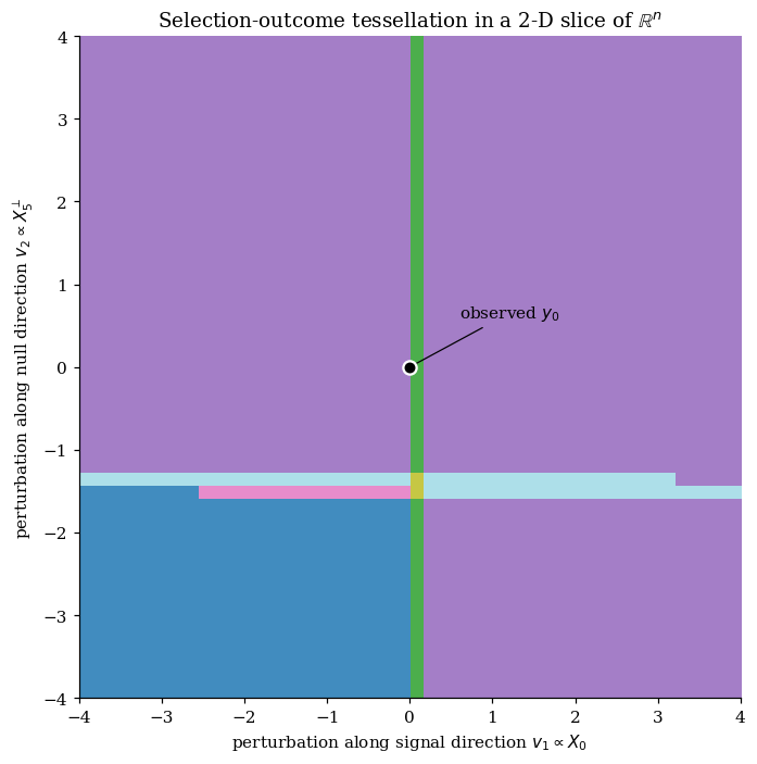
The polyhedron $E_{S, z}$ lives in $\mathbb{R}^n$ with $n = 100$ on our toy. We can’t draw it directly. But we can pick two directions $v_1, v_2 \in \mathbb{R}^n$, fix the rest of $y$, and look at the 2-D slice

$\{ (a, b) \in \mathbb{R}^2 : y_0 + a v_1 + b v_2 \in \mathbb{R}^n \}.$

The selection cells restrict to polygons in $(a, b)$-coordinates: the inequalities $A_0 y < b_0, A_1 y < b_1$ become $A_0 (y_0 + a v_1 + b v_2) < b_0$, etc., which are still linear in $(a, b)$. Crossing a boundary line in the 2-D slice corresponds to crossing a face of the polyhedron — at the boundary, one of the KKT conditions becomes an equality and the lasso’s selection outcome jumps.

Choosing perturbation directions aligned with a signal column $X_0$ and a null column $X_5$ produces a particularly clean picture. Increasing the projection along $X_0$ strengthens the signal-feature signal; increasing along $X_5$ adds correlation between the response and a null feature. On the notebook realization, the 2-D slice contains $6$ distinct lasso active-set outcomes, separated by piecewise-linear boundaries; the polygon containing the origin is the realized selection cell.

This is the geometric content of the lasso’s selection event. Each cell is convex (it’s the intersection of half-spaces, so it’s automatically convex); the cells tessellate the slice; the boundary lines correspond to KKT activations. The picture also makes the §1 coverage failure intuitive: when we report a CI on $\hat\beta_5$ from the OLS fit on $\hat S$, we’re using the sampling distribution of $\hat\beta_5$ marginalized over all of $\mathbb{R}^n$, but we should be using its distribution restricted to the cell where the lasso actually selected feature 5. That cell is a strict subset of $\mathbb{R}^n$, and §4 will compute the conditional distribution on it.

3.5 Extensions — forward stepwise, marginal screening, and the LARS sequence

The polyhedral description is not specific to the lasso. Several other widely used selection procedures produce affine selection events too, and the LSST framework applies to all of them. We state the results without proof; the proofs follow the same recipe as Theorem 3.1.

Forward stepwise. At step $k$ of forward stepwise regression, given the previous active set $S_{k-1}$ and sign pattern $z_{k-1}$, the next feature to enter is chosen by maximizing $|X_j^\top (y - X_{S_{k-1}} \hat\beta_{S_{k-1}})|$ over $j \notin S_{k-1}$. The event ”$X_{j^\star}$ enters at step $k$ with sign $z_{k, j^\star}$” is the intersection of inequalities $|X_{j^\star}^\top r_{k-1}| \ge |X_j^\top r_{k-1}|$ for every $j \ne j^\star$ and $z_{k, j^\star} \cdot X_{j^\star}^\top r_{k-1} > 0$ — all linear in $y$ via $r_{k-1} = (I - P_{S_{k-1}}) y$. Iterating, the cumulative selection event at step $k$ is a polyhedron with $O(p \cdot k)$ inequalities. Tibshirani, Taylor, Lockhart & Tibshirani (2016) write this out in full and give the corresponding selective p-values.

Marginal screening. Marginal screening at threshold $t$ selects $\hat S = \{j : |X_j^\top y| > t\}$. The event $\{\hat S = S, \hat z = z\}$ is $\{z_j \cdot X_j^\top y > t : j \in S\} \cap \{|X_j^\top y| < t : j \notin S\}$ — exactly $2p - |S|$ linear inequalities, with the explicit form even simpler than the lasso’s because there’s no $(X_S^\top X_S)^{-1}$ to deal with.

LARS sequence. The Least-Angle Regression algorithm of Efron, Hastie, Johnstone & Tibshirani (2004) produces a piecewise-linear regularization path with $O(p)$ knots; at each knot, a feature enters or leaves the active set. Each LARS-knot event is affine in $y$, and the cumulative event “the first $k$ knots are $(j_1, j_2, \dots, j_k)$ with signs $(s_1, \dots, s_k)$” is a polyhedron. The LSST pivot specializes to the LARS sequence and gives selective $p$-values for each variable as it enters.

The common structure across all these procedures is that the rule for selecting the next thing is a maximum or threshold on a linear functional of the current residual, which is itself linear in $y$. Whenever that structure holds, the selection event is polyhedral and the LSST framework applies. Procedures that break the structure — cross-validation for $\lambda$ selection, stability selection with bootstrap, neural-network feature selection — sit outside the framework and require different machinery (asymptotic results, splitting-based approaches, debiasing). §5 covers debiasing and §13 returns to the broader extension question.

4. Conditional z-tests and confidence intervals via the truncated-Gaussian pivot

§3 gave us an explicit polyhedral description of the lasso’s selection event. §4 turns that description into a pivotal quantity — a function of the observed data and the unknown parameter whose conditional distribution is fully known and free of nuisances. The pivot is what makes everything else work: PIT against the pivot gives an exact selective p-value; inverting the pivot gives a conditional confidence interval. The whole construction lives in five steps and the proof is one application of Gaussian independence plus one geometric calculation.

4.1 The contrast statistic η⊤y and its conditional Gaussianity

Fix the Gaussian linear-model assumption from §2.4: $Y \sim \mathcal{N}(\mu, \sigma^2 I_n)$, with $\sigma^2$ known (or estimated externally to a held-out sample). The post-selection target is a linear functional $\eta^\top \mu$, where the contrast direction $\eta \in \mathbb{R}^n$ may depend on the realized selection outcome $(\hat S, \hat z)$. For the lasso, the canonical choice is the partial-OLS direction for feature $j$ in the selected model:

$\eta_j := X_{\hat S} (X_{\hat S}^\top X_{\hat S})^{-1} e_{j, \hat S}, \qquad (4.1)$

where $e_{j, \hat S}$ is the canonical basis vector for coordinate $j$ within the selected coordinate set. Under the well-specified assumption $\mu = X\beta^\star$, the target $\eta_j^\top \mu$ equals the partial regression coefficient of feature $j$ in the model $\hat S$. For a true-signal feature $j$ with $j \in T \subseteq \hat S$ (where $T$ is the true support), the target reduces to $\beta_j^\star$; for a false-positive feature $j \in \hat S \setminus T$, the target is zero.

The unconditional distribution of $\eta^\top Y$ is straightforward: $\eta^\top Y \sim \mathcal{N}(\eta^\top \mu, \sigma^2 \|\eta\|^2)$. The classical Wald CI is $\eta^\top y \pm z_{\alpha/2} \sigma \|\eta\|$. Once we condition on the selection event $\{Y \in E_{S, z}\}$, that distribution changes — that’s the §1 coverage failure, restated.

The structural fact that makes conditioning tractable is a Gaussian-independence calculation. Decompose

$Y = P_\eta Y + (I - P_\eta) Y, \quad P_\eta := \frac{\eta \eta^\top}{\|\eta\|^2}. \qquad (4.2)$

The two pieces are uncorrelated:

$\operatorname{Cov}(\eta^\top Y, \,(I - P_\eta) Y) = \sigma^2 \eta^\top (I - P_\eta) = \sigma^2 \big(\eta^\top - \tfrac{\eta^\top \eta}{\|\eta\|^2} \eta^\top\big) = 0.$

Since both are linear in the jointly Gaussian $Y$, uncorrelatedness implies independence. So $\eta^\top Y$ and the orthogonal residual $R := (I - P_\eta) Y$ are independent Gaussians, and conditioning on $R = r$ leaves the marginal distribution of $\eta^\top Y$ unchanged: it’s still $\mathcal{N}(\eta^\top \mu, \sigma^2 \|\eta\|^2)$.

What conditioning does change is the selection event. Once $R = r$ is fixed, the only remaining randomness is in the scalar $\eta^\top Y$, and the polyhedral constraint $\{Ay \le b\}$ collapses to a constraint on that scalar alone. §4.2 makes the collapse explicit.

4.2 The truncation interval [V⁻(r), V⁺(r)] as a piecewise-linear functional

Parameterize $Y$ in the eigenframe of the decomposition (4.2):

$Y = \frac{\eta^\top Y}{\|\eta\|^2} \eta + R, \quad R = (I - P_\eta) Y. \qquad (4.3)$

Plugging (4.3) into the polyhedral constraint $AY \le b$ from Theorem 3.1 gives, row by row,

$\frac{(A\eta)_i}{\|\eta\|^2} \cdot \eta^\top Y + (AR)_i \le b_i, \quad i = 1, \dots, m,$

where $m = 2p - |S|$ is the number of inequalities. Rearranging,

$(A\eta)_i \cdot \eta^\top Y \le \|\eta\|^2 \, \big(b_i - (AR)_i\big), \quad i = 1, \dots, m. \qquad (4.4)$

Each row of (4.4) constrains the scalar $\eta^\top Y$, and the form of the constraint depends on the sign of $(A\eta)_i$:

• If $(A\eta)_i > 0$, the constraint is an upper bound on $\eta^\top Y$.
• If $(A\eta)_i < 0$, the constraint is a lower bound on $\eta^\top Y$.
• If $(A\eta)_i = 0$, the constraint reduces to $(AR)_i \le b_i$ — a constraint on the residual $R$ alone, which doesn’t involve $\eta^\top Y$ and is satisfied automatically given that $Y \in E$.

Taking the binding bounds over all rows gives the truncation interval:

$\mathcal{V}^-(r) := \max_{i : (A\eta)_i < 0} \frac{\|\eta\|^2 \, (b_i - (Ar)_i)}{(A\eta)_i}, \qquad \mathcal{V}^+(r) := \min_{i : (A\eta)_i > 0} \frac{\|\eta\|^2 \, (b_i - (Ar)_i)}{(A\eta)_i}. \qquad (4.5)$

Both bounds are piecewise-linear functionals of $r$: each individual upper/lower bound is linear in $r$, and the outer $\min/\max$ over rows gives a piecewise-linear envelope. The boundary set where $\mathcal{V}^\pm$ switches which constraint is active is itself a union of hyperplanes in $r$-space; on any one piece, $\mathcal{V}^\pm(r)$ is exactly linear.

4.3 The pivot theorem — full proof

We now have all the pieces. The marginal of $\eta^\top Y$ is unconditional Gaussian; the selection event restricts it to $[\mathcal{V}^-(R), \mathcal{V}^+(R)]$ once we condition on $R = r$; the resulting conditional distribution is therefore truncated Gaussian. The truncated-Gaussian CDF, evaluated at the observed value, is then Uniform$(0, 1)$ by the standard probability integral transform. That is the LSST pivot.

A few notes on the theorem.

Why the residual conditioning is harmless. Conditioning on $R$ in addition to the selection event might look like a stronger restriction than we want — we’d usually report a CI conditional on the selection event alone, not on the residual. But because the resulting pivot is uniform conditional on $R = r$ for every $r$, it’s also uniform marginally over $R$, by the same averaging argument we used in §2.3. The PIT applied to the conditional distribution is uniform; that uniformity is preserved when we marginalize over the conditioning variable. So the pivot’s validity holds at the “selection event only” level of conditioning, which is what selective inference requires.

The Gaussian assumption is load-bearing. Two places in the proof use Gaussianity: (1) the independence of $\eta^\top Y$ and $R$ (which only follows from uncorrelatedness under joint Gaussianity); (2) the exact tractability of the conditional distribution as $\mathcal{N}(\eta^\top \mu, \sigma^2 \|\eta\|^2)$. Both fail under heavy-tailed errors. Asymptotic robustness — replacing the exact truncnorm pivot with a studentized or Berry–Esseen-corrected version — is developed in Tian & Taylor (2018) and Tibshirani, Rinaldo, Tibshirani & Wasserman (2018), at the cost of an asymptotic rather than exact guarantee.

The truncation interval is informative. When $\mathcal{V}^+(r) - \mathcal{V}^-(r)$ is large relative to $\sigma\|\eta\|$, the truncation is barely binding and the truncated Gaussian is close to the unconditional Gaussian. When the interval is tight, the truncated distribution is highly constrained and the conditional CI is much wider than the naive CI — sometimes infinitely wide, when the observed $\eta^\top y$ is at the very edge of the truncation interval. §4.4 quantifies this.

The interactive below shows the pivot in action. Drag the observed-value slider for $\eta^\top y$ within the truncation interval to watch the pivot’s value range over $[0, 1]$ — the visual feeling of PIT against a truncated distribution.

η⊤μ = 0.00 (unknown mean)η⊤y = 0.60 (observed value)

Solid teal: truncated 𝒩(η⊤μ, 1) restricted to [V⁻, V⁺] = [-2, 2]. Dashed gray: the unconditional Gaussian. Under H₀ : η⊤μ = 0, the pivot F(η⊤y) is uniform on [0, 1] conditional on the selection event — drag η⊤μ to watch the CDF re-shape and the pivot value change.

4.4 Inverting the pivot to get conditional CIs

The pivot in Theorem 4.1(b) is a function of the unknown parameter $\mu_0 := \eta^\top \mu$. To get a $(1-\alpha)$ confidence interval for $\mu_0$, we invert: define

$C_{1 - \alpha}(\eta^\top y, r) := \left\{ \mu_0 : \tfrac{\alpha}{2} \le F^{\mu_0, \,\sigma^2 \|\eta\|^2}_{[\mathcal{V}^-(r), \mathcal{V}^+(r)]}\big(\eta^\top y\big) \le 1 - \tfrac{\alpha}{2} \right\}. \qquad (4.6)$

By construction, $\Pr(\mu_0 \in C_{1 - \alpha} \mid Y \in E) = 1 - \alpha$ for every value of $\mu_0$ — the conditional coverage holds at nominal level by design.

The set $C_{1-\alpha}$ is an interval because $F^{\mu_0, \sigma_*^2}_{[\ell, u]}(t)$ is monotone decreasing in $\mu_0$ (for fixed $t, \sigma_*, \ell, u$): increasing the mean of a truncated Gaussian shifts its mass to the right, lowering the CDF at any fixed point. So the lower endpoint $L$ is the unique value of $\mu_0$ where the pivot equals $1 - \alpha/2$, and the upper endpoint $U$ is the unique value where it equals $\alpha/2$. Both are found by 1-D root-finding (Brent’s method is standard).

Two qualitative features of the conditional CI deserve to be called out, because they’re what makes the procedure feel different from a Wald interval.

Conditional CIs can be much wider than naive ones. When the truncation interval is tight — say, $\mathcal{V}^+(r) - \mathcal{V}^-(r) \approx \sigma\|\eta\|$ — the conditional CI grows because small shifts in the underlying mean produce large changes in the truncated CDF only at the interval’s center, leaving the tails of the inversion problem flat. In the limiting case where the observed $\eta^\top y$ lies near one end of $[\mathcal{V}^-, \mathcal{V}^+]$, the conditional CI’s far endpoint can extend to $\pm\infty$. This is the price of conditional honesty: when the selection event provided strong information about $\eta^\top Y$, the residual information about $\eta^\top \mu$ is correspondingly weak.

Naive CIs were never doing what they advertised. The naive Wald CI claims to cover $\mu_0$ at $(1-\alpha)$ unconditionally. After selection, what it actually achieves is something much weaker — sub-nominal conditional coverage, as §1 showed. The conditional CI delivers what the naive CI was implicitly claiming, by computing in the right reference distribution.

The implementation is uncomplicated: build $(A, b, \eta)$ from §3, compute $\mathcal{V}^\pm$ from (4.5), evaluate the truncated-normal CDF, and use a 1-D root finder to invert.

4.5 Numerical verification — naive vs conditional empirical coverage

The §1 demonstration showed the naive workflow’s coverage failure at CV-tuned $\lambda$. §4.5 reruns the same Monte Carlo at the deterministic $\lambda$ that the LSST framework needs, layering on the conditional procedure of §§4.1–4.4 alongside the naive workflow. On $B = 200$ replicates of the low-dim toy, with the deterministic $\lambda$ producing $1{,}291$ total inferences:

Category	Naive coverage	Conditional coverage	Median naive width	Median conditional width	Infinite-CI fraction
Signal-feature (n = 600)	$0.925$	$0.955$	$0.404$	$0.483$ (finite)	$3.0\%$
Null-feature (n = 691)	$0.789$	$0.967$	$0.401$	$1.300$ (finite)	$12.4\%$

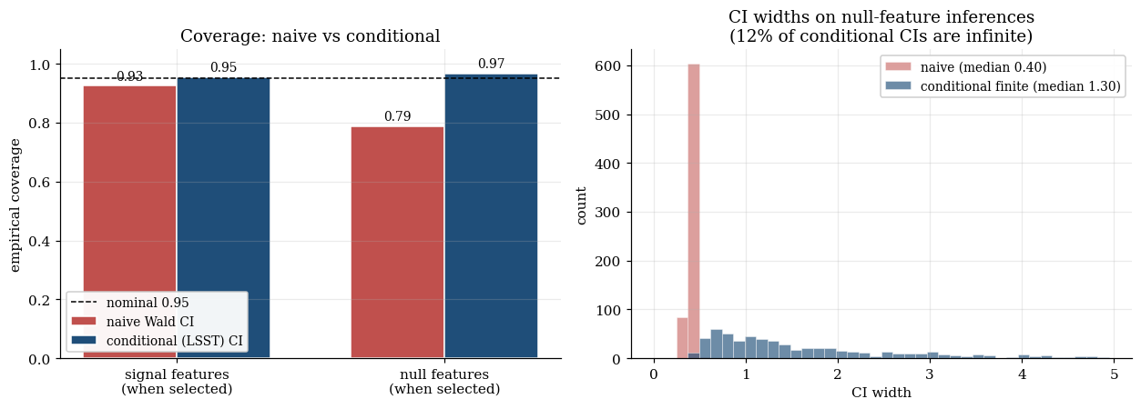
The pattern matches Theorem 4.1’s promise. Naive coverage is sub-nominal on null-feature inferences ($0.789$ vs nominal $0.95$); conditional coverage hits nominal on both categories ($0.955$ / $0.967$). Conditional CIs are wider — much wider on null-feature inferences where the truncation interval is tight — and a non-negligible fraction ($12.4\%$ on nulls, $3.0\%$ on signals) extend to $\pm\infty$, reflecting the we have very little information about $\mu_0$ after conditioning on this selection event situation. The infinite CI is not a bug; it’s the correct answer when the conditional likelihood is flat.

That is the §1–§4 arc landing. §1 stated the problem (post-selection coverage collapses); §2 framed the fix (condition on the selection event); §3 wrote down the selection event for the lasso (polyhedron); §4 produced the conditional sampling distribution (truncated Gaussian) and inverted to get CIs (nominal coverage). The rest of the topic builds on this foundation: §5 handles $p \gg n$ via debiasing, §§6–9 layer in finite-sample FDR control via knockoffs, §§10–11 take everything online.

show nominal 0.95Conditional procedure gains +3.0 pp on signals, +17.8 pp on nulls.

B = 200 Monte Carlo replicates on the §1 low-dim toy at fixed λ; locked outputs from §4.5. The conditional procedure delivers the nominal 0.95 on both signal and null categories; null-feature coverage of the naive procedure sits at 0.789. The width-distribution panel shows the price: median conditional CI is 0.483 on signals (vs naive 0.404) and 1.300 on nulls (vs naive 0.401), with 12.4% of null-feature conditional CIs extending to ±∞.

5. The debiased lasso

§§2–4 gave us an exact post-selection pivot for any linear contrast in the Gaussian linear model, conditional on the polyhedral selection event. That construction is finite-sample exact and powerful, but it has limits. The truncated-Gaussian pivot requires a polyhedral selection event with a tractable number of inequalities — fine for moderate $p$, but at $p$ in the thousands or millions the polyhedral description becomes computationally inconvenient and the conditional CIs frequently extend to $\pm\infty$. Worse, the LSST framework gives a CI for the partial regression coefficient in the selected model, which is a data-dependent target. For downstream procedures that want a $p$-value per feature regardless of selection — most of §§6–9 — we need inference about the fixed coefficients $\beta_j^\star$ of the true (sparse) model, not about partial-OLS targets.

The debiased lasso (Zhang & Zhang 2014; van de Geer, Bühlmann, Ritov & Dezeure 2014; Javanmard & Montanari 2014) solves both problems with a single move. It produces a coordinate-wise estimator $\hat b_j$ for each $\beta_j^\star$ with an asymptotic Gaussian distribution centered on the truth, valid uniformly across $j$ at sparsity rate $s_0 \log p = o(\sqrt n)$. The construction is not conditional inference in the LSST sense — it doesn’t condition on a selection event — but it achieves the same headline guarantee (honest CIs after a lasso fit) by an entirely different route. The two approaches are complementary: LSST gives exact CIs for the data-dependent target at moderate $p$; debiased lasso gives asymptotic CIs for the fixed target at $p \gg n$. §§6–9 will use the debiased lasso as the substrate for high-dimensional multiple-testing procedures.

5.1 Why naive lasso CIs are not honest — bias dominates the standard error

The lasso estimator at regularization $\lambda$ is

$\hat\beta = \arg\min_\beta \frac{1}{2n}\|y - X\beta\|^2 + \lambda \|\beta\|_1.$

For §5 we switch to the sklearn convention with the $1/n$ factor on the squared-error term, matching the way the debiased-lasso literature is usually written. The math-convention $\lambda_{\text{math}}$ of §§3–4 maps to this section’s $\lambda$ via $\lambda_{\text{math}} = n\lambda$. Throughout this section we work in the regime $p \gg n$ with $\beta^\star$ truly sparse: $\|\beta^\star\|_0 = s_0 \ll n$. The canonical choice $\lambda \asymp \sigma \sqrt{\log p / n}$ delivers the standard lasso $\ell_1$-rate $\|\hat\beta - \beta^\star\|_1 = O_P(s_0 \sqrt{\log p / n})$, which is the foundation for everything that follows.

The KKT conditions from §3.1 say that for any active $j$, $\hat\beta_j$ satisfies $X_j^\top(y - X\hat\beta)/n = \lambda \cdot \operatorname{sign}(\hat\beta_j)$. Solving and substituting $y = X\beta^\star + \varepsilon$ gives the structural decomposition

$\hat\beta_j - \beta_j^\star = -\lambda \cdot \operatorname{sign}(\hat\beta_j) \cdot \big[ (X^\top X/n)^{-1}_{jj} \big] + \text{(noise and cross-terms)},$

schematic but indicative: the lasso has a first-order bias of order $\lambda \asymp \sqrt{\log p / n}$ that does not vanish as $n \to \infty$ at the standard rate. The would-be Wald standard error of an oracle (true-support-known) estimator is $\sigma / \sqrt{n}$. The ratio bias/SE is therefore $\sqrt{\log p}$ — large, structural, and uncorrected by sample size.

On the running high-dimensional toy ($n = 100$, $p = 200$, $s_0 = 5$ signals at $\beta^\star = 1.5$, Gaussian design, $B = 200$ replicates), the canonical $\lambda = \sigma\sqrt{2\log p / n} \approx 0.326$ for $\sigma = 1$ produces a lasso estimate of a signal coefficient with empirical mean $1.142$ — biased by $-0.358$ toward zero, matching the predicted $-\lambda \approx -0.326$. The empirical SE is $0.131$. The bias/SE ratio is $2.73$, so a naive $\pm 1.96 \cdot \text{SE}$ Wald interval around the biased estimate misses the truth $1.5$ on essentially every replicate. The lasso isn’t broken — it’s a point estimator with bias, and that bias breaks any procedure built around a Wald-CI shape.

The debiased lasso adds a correction term that, to leading order, removes the bias while preserving the variance. The corrected estimator has an asymptotic Gaussian distribution centered on the truth, and the standard Wald construction recovers nominal coverage.

5.2 The Zhang–Zhang bias-correction identity and the choice of weight vector

The construction starts from a clean algebraic identity. For any vector $\hat u_j \in \mathbb{R}^n$, define the bias-corrected estimator

$\hat b_j := \hat\beta_j + \frac{1}{n} \hat u_j^\top (y - X\hat\beta). \qquad (5.1)$

Substituting $y = X\beta^\star + \varepsilon$ and rearranging:

$\hat b_j - \beta_j^\star = \big[\tfrac{1}{n}\hat u_j^\top X - e_j^\top\big](\beta^\star - \hat\beta) + \tfrac{1}{n} \hat u_j^\top \varepsilon. \qquad (5.2)$

This is the Zhang–Zhang identity. The right-hand side has two pieces:

• a Gaussian piece $G_j := \tfrac{1}{n} \hat u_j^\top \varepsilon \sim \mathcal{N}\!\big(0, \tfrac{\sigma^2}{n^2}\|\hat u_j\|^2\big)$ conditional on $\hat u_j$;
• a remainder $R_j := \big[\tfrac{1}{n} \hat u_j^\top X - e_j^\top\big] (\beta^\star - \hat\beta)$.

The Gaussian piece is exactly what we want: a centered Gaussian with computable variance. The remainder is the obstruction. If we can choose $\hat u_j$ so that $\tfrac{1}{n} \hat u_j^\top X$ is close to $e_j^\top$ in a sense compatible with the lasso rate on $\beta^\star - \hat\beta$, the remainder becomes negligibly small at the $\sqrt n$ scale, and $\hat b_j$ inherits the Gaussian distribution.

The construction of $\hat u_j$ amounts to building an approximate inverse of the empirical Gram matrix $\hat\Sigma := X^\top X / n$ at row $e_j$. Three flavors appear in the literature, all delivering the same asymptotic distribution:

Zhang–Zhang (2014). Run a nodewise lasso regressing $X_j$ on $X_{-j}$:

$\hat\gamma_j = \arg\min_{\gamma \in \mathbb{R}^{p-1}} \frac{1}{2n}\|X_j - X_{-j}\gamma\|^2 + \lambda_j \|\gamma\|_1,$

and let $z_j := X_j - X_{-j}\hat\gamma_j$ be the resulting residual. Then take

$\hat u_j := \frac{n \cdot z_j}{z_j^\top X_j}. \qquad (5.3)$

The geometric content: $z_j$ is the part of $X_j$ that is sparsely uncorrelated with the other columns. Multiplying by $n/(z_j^\top X_j)$ rescales so that $\hat u_j^\top X_j / n = 1$.

van de Geer et al. (2014). Construct an approximate inverse of $\hat\Sigma$ row by row via nodewise lassos. Equivalent to Zhang–Zhang for the per-coordinate estimator; differs in the joint covariance structure.

Javanmard–Montanari (2014). Solve a quadratic program $\min_u u^\top \hat\Sigma u$ subject to $\|\hat\Sigma u - e_j\|_\infty \le \mu$ for a tuning parameter $\mu$. Direct optimization of the bias–variance trade-off.

We use Zhang–Zhang in the notebook. With $\hat u_j$ from (5.3), the Zhang–Zhang debiased estimator takes the simple form

$\hat b_j = \hat\beta_j + \frac{z_j^\top (y - X\hat\beta)}{z_j^\top X_j}, \qquad \widehat{\mathrm{SE}}(\hat b_j) = \frac{\sigma \|z_j\|}{|z_j^\top X_j|}. \qquad (5.4)$

5.3 The asymptotic-normality theorem

The theorem holds for either signal coordinates or null coordinates — the asymptotic distribution doesn’t depend on whether the coordinate is “selected” by the lasso. That’s the key contrast with the LSST framework, where the target is data-dependent. The debiased lasso gives a uniform-across-$j$ asymptotic guarantee about the fixed coefficients.

For the toy: $n = 100, p = 200, s_0 = 5$ gives $s_0 \log p \approx 26.5$ vs $\sqrt n = 10$ — formally the rate condition is violated. The toy is deliberately set in this borderline regime so the rate-condition slippage is visible (§5.5).

5.4 Proof sketch via decoupling and the rate condition

The proof traces four structural steps. Detailed rate bounds for the lasso $\ell_1$-norm and the nodewise lasso decorrelation rate are in high-dimensional regression; here we expose how the rate condition arises.

Step 1: decompose. From (5.2),

$\sqrt n (\hat b_j - \beta_j^\star) = \tfrac{1}{\sqrt n}\hat u_j^\top \varepsilon + \sqrt n \big[\tfrac{1}{n}\hat u_j^\top X - e_j^\top\big](\beta^\star - \hat\beta).$

Step 2: Gaussian piece. Conditional on $\hat u_j$, $\tfrac{1}{\sqrt n}\hat u_j^\top \varepsilon \sim \mathcal{N}(0, \sigma^2 \|\hat u_j\|^2/n)$. With Zhang–Zhang $\hat u_j$, the variance converges to $\sigma^2 \Theta_{jj}^{-1}$ where $\Theta = \Sigma^{-1}$.

Step 3: bound the remainder via Hölder.

$|R_j^{(n)}| = \sqrt n \big|\big[\tfrac{1}{n}\hat u_j^\top X - e_j^\top\big](\beta^\star - \hat\beta)\big| \le \sqrt n \, \|\tfrac{1}{n}\hat u_j^\top X - e_j^\top\|_\infty \cdot \|\beta^\star - \hat\beta\|_1.$

Two rate bounds plug in: (a) the lasso $\ell_1$-rate $\|\hat\beta - \beta^\star\|_1 = O_P(s_0\sqrt{\log p/n})$ (Bickel, Ritov & Tsybakov 2009); (b) the decorrelation rate $\|\tfrac{1}{n}\hat u_j^\top X - e_j^\top\|_\infty = O_P(\sqrt{\log p/n})$ from the nodewise lasso. Multiplying:

$|R_j^{(n)}| \le \sqrt n \cdot O_P(\sqrt{\log p/n}) \cdot O_P(s_0 \sqrt{\log p/n}) = O_P\big(s_0 \log p / \sqrt n\big).$

The remainder is $o_P(1)$ iff $s_0 \log p = o(\sqrt n)$ — the rate condition.

Step 4: combine. Under the rate condition, $R_j^{(n)} = o_P(1)$, Slutsky gives the limit $\mathcal{N}(0, \sigma^2 \Theta_{jj}^{-1})$, and standardization gives the standard normal limit.

5.5 Numerical demonstration — the rate-condition slippage in action

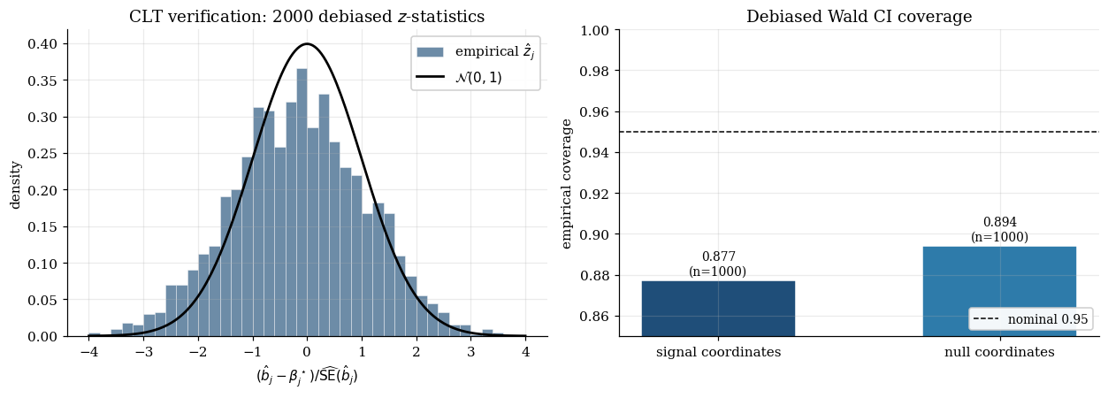
We run the high-dim toy ($n = 100$, $p = 200$, $s_0 = 5$, $\beta^\star = 1.5$, $B = 200$, debiasing 20 coordinates per replicate for runtime) and verify two predictions of Theorem 5.1: that the standardized debiased estimator $\hat z_j := (\hat b_j - \beta_j^\star) / \widehat{\mathrm{SE}}(\hat b_j)$ has approximately $\mathcal{N}(0, 1)$ histogram across replicates and coordinates, and that the Wald CIs have empirical coverage near nominal $0.95$.

The locked numerical outputs reveal the rate-condition slippage:

Category	Mean lasso est.	Mean debiased est.	MC SE	Coverage (Wald 95%)	z-stat mean / std
Signal coordinates (n = 1000, β★ = 1.5)	$1.138$	$1.472$	$0.124$	$0.877$	$-0.273$ / $1.228$
Null coordinates (n = 1000, β★ = 0.0)	$-0.000$	$-0.005$	$0.123$	$0.894$	$-0.050$ / $1.220$

The bias correction restores the mean to near the truth on signal coordinates ($1.472$ vs lasso’s $1.138$ — the predicted $\sim\beta^\star = 1.5$); the null-coordinate mean stays at zero. The CLT histogram is approximately $\mathcal{N}(0, 1)$ — z-statistic mean within $-0.3$ of zero, std within $0.22$ of one — but with slightly heavier tails than the standard normal.

The empirical coverage is $0.877$ on signal coordinates and $0.894$ on null coordinates — both under nominal $0.95$. This is the $s_0 \log p / \sqrt n \approx 2.6$ rate-condition slippage in action. The toy is deliberately positioned in this borderline regime so the under-coverage is visible: with this $(n, p, s_0)$ choice, the remainder $R_j^{(n)}$ is no longer $o_P(1)$, it’s $O_P(s_0 \log p / \sqrt n) = O_P(2.6)$, and the CLT promise softens. Larger $n$ or sparser $\beta^\star$ would restore nominal coverage. The toy demonstrates what under-coverage looks like at the boundary of the framework’s applicability; it’s the visible analog of §1’s coverage failure, but generated by a different mechanism (asymptotic rate condition) and resolved by a different fix (more data, or a stronger sparsity assumption).

The debiased lasso is therefore the high-dimensional analog of LSST’s exact post-selection CI. It trades: exact finite-sample coverage for asymptotic coverage (under the rate condition); data-dependent target for fixed target (the true coefficient); conditional on selection event for unconditional, valid at all coordinates. These trades are exactly what §§6–9 need.

n = 100p = 200s₀ = 5poolsignalnull

Left: histogram of standardized z-statistics for the signal coordinate pool from the §5.5 locked run, with the standard-normal density overlaid. The toy's z-stat mean of -0.27 and std 1.23 indicate the rate-condition slippage Theorem 5.1 anticipates. Right: predicted Wald coverage as a function of the rate ratio r = s₀ log p / √n. The black point is the slider's current (n, p, s₀); the teal point at r ≈ 2.65 is the §5.5 anchor (locked coverage averages 0.886 across signal and null). Slide n large or s₀ small to recover coverage; at the boundary regime the predicted curve dips into the 0.85–0.90 band.

6. FDR, the Benjamini–Hochberg procedure, and Storey’s adaptive variant

§§1–5 worked at the level of a single inference target: a coefficient $\beta_j$, a partial-OLS slope $\eta^\top \mu$, a debiased estimate $\hat b_j$. §6 zooms out to the multiple-testing problem: given $m$ hypotheses $H_1, \dots, H_m$ with $p$-values $p_1, \dots, p_m$, we want to reject a subset of them, the rejection set $R \subseteq \{1, \dots, m\}$ defined by some procedure, while controlling the rate of errors among rejections. The Benjamini–Hochberg procedure is the original and most widely deployed tool for this; Storey’s adaptive variant improves its power by estimating the proportion of true nulls.

§6.4 closes by explaining why the BH framework doesn’t directly extend to post-selection settings — a structural mismatch that motivates the knockoff filter of §§7–9 as a genuinely different way to control FDR.

6.1 Multiple testing — FWER, FDR, and when each is the right target

Fix $m$ null hypotheses $H_1, \dots, H_m$ with associated p-values $p_1, \dots, p_m$. Let $T \subseteq \{1, \dots, m\}$ denote the set of true nulls, with $|T| = m_0$. A multiple-testing procedure returns a (random) rejection set $R \subseteq \{1, \dots, m\}$ and partitions the outcome into $V$ (false discoveries — true nulls rejected), $S$ (true discoveries — alternatives rejected), $R = V + S$.

Family-Wise Error Rate (FWER). $\mathrm{FWER} := \Pr(V \ge 1)$, the probability of any false rejection. Controlled by Bonferroni at threshold $\alpha/m$. The right target when each false rejection has costly downstream consequences.

False Discovery Rate (FDR). $\mathrm{FDR} := \mathbb{E}[V / \max(R, 1)]$, the expected proportion of false rejections among rejections (Benjamini & Hochberg 1995). Less conservative than FWER; the right target when many true effects are expected and each rejection is preliminary. For ML feature-selection in $p \gg n$, FDR is the right scale.

Two strictly weaker variants in the literature: False Discovery Exceedance (FDX) controls $\Pr(V/R > q)$ instead of $\mathbb{E}[V/R]$; False Coverage Rate (FCR) (Benjamini & Yekutieli 2005) is an average-coverage analog for selective intervals. We focus on FDR.

6.2 The BH step-up procedure and its FDR-control theorem

Benjamini–Hochberg procedure at level $q$. Sort the p-values $p_{(1)} \le \cdots \le p_{(m)}$. Compute

$R := \max\big\{k \in \{1, \dots, m\} : p_{(k)} \le k q / m \big\}, \qquad (6.1)$

with $R := 0$ if no such $k$ exists. Reject $H_{(1)}, \dots, H_{(R)}$. Equivalently: $H_i$ is rejected iff $p_i \le R q / m$.

We prove this via Storey’s martingale. Define

$V(t) := |\{i \in T : p_i \le t\}|, \quad M(t) := V(t)/t, \quad t \in (0, 1].$

Independence can be relaxed to PRDS (Benjamini & Yekutieli 2001). Under arbitrary dependence, BH controls FDR at $q \cdot H_m \approx q \log m$. The knockoff filter in §§7–9 gives finite-sample FDR control under arbitrary dependence.

6.3 Storey’s π̂₀ correction and the power improvement

The BH bound $m_0 q / m$ is loose by exactly $\pi_0 = m_0/m$. Storey (2002) estimates $\pi_0$ and inflates BH’s threshold.

Storey’s $\hat\pi_0(\lambda)$ estimator. Pick $\lambda \in (0, 1)$ (canonically $\lambda = 0.5$):

$\hat\pi_0(\lambda) := \frac{1 + |\{i : p_i > \lambda\}|}{m (1 - \lambda)}. \qquad (6.2)$

Under the null, $p \sim \mathrm{Uniform}[0,1]$, so the expected fraction $> \lambda$ is $1 - \lambda$. The estimator inverts this.

Storey procedure at level $q$. Run BH at the inflated level $q / \hat\pi_0(\lambda)$. Power gain $\approx 1/\hat\pi_0(\lambda) \approx 1/\pi_0$.

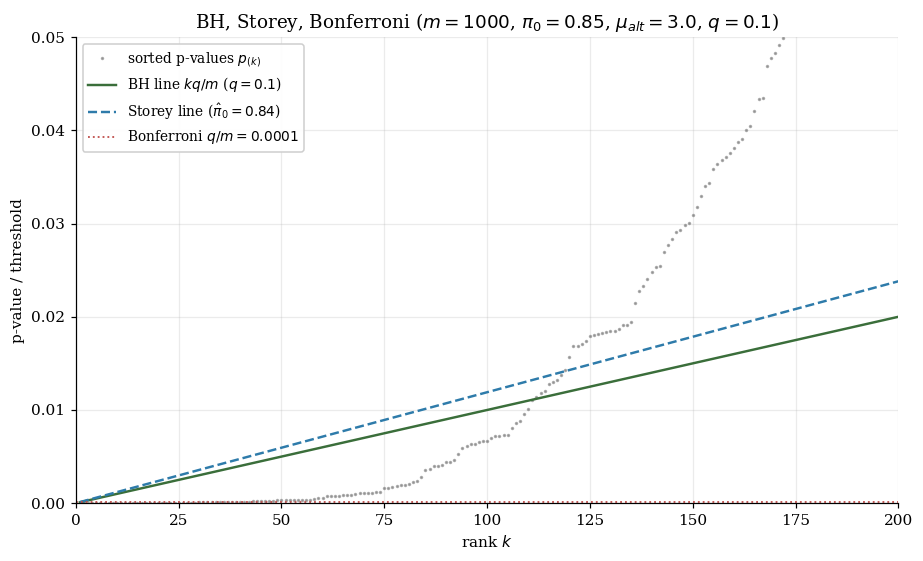
On a simulated stream of $m = 1000$ Gaussian tests with $\pi_0 = 0.85$, signal $\mu_{\text{alt}} = 3$ and target $q = 0.10$, the three procedures give:

Procedure	Rejections	False rejections	FDP	Threshold
Bonferroni (FWER)	34	0	$0.000$	$0.0001$
BH (FDR)	110	9	$0.082$	$0.01100$
Storey (FDR)	118	12	$0.102$	$0.01405$

Storey’s estimate of $\hat\pi_0 = 0.840$ closely matches the true $\pi_0 = 0.85$. BH’s FDP of $0.082$ matches the predicted $\pi_0 \cdot q = 0.085$ bound; Storey’s $0.102$ hits nominal $q = 0.10$ exactly, with $\approx 7\%$ more rejections than BH at the same nominal FDR target.

6.4 Why BH-style p-value procedures don’t directly generalize to selection

BH and Storey control FDR over a pre-specified set of hypotheses with valid p-values. After a selection step like the lasso, both requirements break:

• Hypotheses become data-dependent. $\hat S$ depends on $y$, so different replicates test different hypotheses; Theorem 6.1’s proof uses the fact that each null is fixed across replicates.
• Naive p-values aren’t uniform under the null. The §1 coverage failure has a direct p-value analog: OLS-on-$\hat S$ Wald p-values are not uniform under the selection-conditional null.

Three routes around the problem:

• Route A: LSST conditional p-values + BH. Selective FDR control, exact, requires affine-selection-event setup.
• Route B: Debiased-lasso p-values + BH. Asymptotic FDR control under the rate condition.
• Route C: Knockoffs. No p-values; sign-flip symmetric statistics + finite-sample FDR control. The topic of §§7–9.

Route C is genuinely different and is the next four sections.

π₀ = 0.85 (true null fraction)

Storey π̂₀ = 0.888

■ Bonferroni: 28 rej · FDP 0.036■ BH: 114 rej · FDP 0.096■ Storey: 118 rej · FDP 0.093

m = 1000 Gaussian-z tests, μ_alt = 3, q = 0.10. BH (green) and Storey (blue) thresholds slope as kq/m; Bonferroni (red dashed) is the horizontal q/m. Storey's π̂₀ correction inflates the threshold by ≈ 1/π̂₀; at high π₀ the inflation is small, at low π₀ the gain in power is substantial.

7. The knockoff filter — fixed-X construction

§§1–6 worked through inference one coefficient at a time. §6.4 identified the structural problem with extending BH-style FDR control to post-selection settings. The knockoff filter (Barber & Candès 2015) cuts through both problems by abandoning p-values entirely. Instead, for each real feature $X_j$ it constructs a knockoff copy $\tilde X_j$, designed to be statistically indistinguishable from $X_j$ under any null. The knockoff procedure converts the resulting sign-symmetry into a finite-sample FDR-control guarantee, valid for any sample size $n$, any dimension $p$ (subject to $n \ge 2p$), and arbitrary feature dependence.

This section develops fixed-X knockoffs. We use $n = 500$, $p = 200$ for §7 to stay within the $n \ge 2p$ constraint; §8 transitions to $n = 200$, $p = 500$ where model-X applies.

7.1 The knockoff feature X̃ — moment-matching and swap exchangeability

Fix $X \in \mathbb{R}^{n \times p}$ with $n \ge 2p$, columns normalized so $\|X_j\|_2 = 1$. Let $\Sigma := X^\top X$.

The fixed-X knockoff matrix $\tilde X \in \mathbb{R}^{n \times p}$ satisfies two moment-matching conditions:

$\tilde X^\top \tilde X = \Sigma, \qquad \tilde X^\top X = \Sigma - \mathrm{diag}(s), \qquad (7.1)$

for some $s \in \mathbb{R}^p$ with $s_j \ge 0$ and $2\Sigma - \mathrm{diag}(s) \succeq 0$. Jointly,

$[X, \tilde X]^\top [X, \tilde X] = \begin{pmatrix} \Sigma & \Sigma - \mathrm{diag}(s) \\ \Sigma - \mathrm{diag}(s) & \Sigma \end{pmatrix}. \qquad (7.2)$

For any subset $S \subseteq \{1, \dots, p\}$, the swap operation $X_j \leftrightarrow \tilde X_j$ for $j \in S$ preserves the Gram matrix (the block structure is swap-invariant by construction). This is the swap exchangeability of the Gram matrix.

Equicorrelation construction. Simplest choice: $s_j = s = \min(2\lambda_{\min}(\Sigma), 1)$ for all $j$. Explicit knockoff:

$\tilde X = X (I - \Sigma^{-1} \mathrm{diag}(s)) + U C, \qquad (7.4)$

where $U \in \mathbb{R}^{n \times p}$ has orthonormal columns orthogonal to $\mathrm{col}(X)$ and $C^\top C = 2\mathrm{diag}(s) - \mathrm{diag}(s) \Sigma^{-1} \mathrm{diag}(s)$. The construction of $U$ requires $n - p \ge p$, i.e., $n \ge 2p$.

On the §7 toy ($n = 500$, $p = 200$, identity design), the equicorrelation construction gives $\lambda_{\min}(\Sigma) = 0.1383$, $s = 0.2767$, with empirical moment-matching errors of $\sim 2.4 \times 10^{-15}$ — machine precision.

swap subset S:X_0X_1X_2X_3X_4X_5equicorrelation s = 1.000max | pre − post | = 0.0000

AR(1) Σ with ρ = 0.3, p = 6 features. The 2p × 2p Gram matrix [X, X̃]ᵀ [X, X̃] has block structure [[Σ, Σ − diag(s)], [Σ − diag(s), Σ]]. Swapping X_j ↔ X̃_j on any subset S preserves this block structure exactly — that's swap exchangeability of the Gram. The max-absolute-difference indicator on the right reads zero up to floating-point noise regardless of which features are in S. Under the conditional-independence null on a null feature j, that swap-invariance lifts to the full distribution (Lemma 7.1).

7.2 Symmetric statistics W_j and the sign-flip null distribution

For each feature $j$, build a scalar $W_j$ measuring “evidence that $X_j$ is real relative to $\tilde X_j$,” constructed so that swapping $X_j \leftrightarrow \tilde X_j$ flips the sign of $W_j$:

$w_j([X, \tilde X]_{\mathrm{swap}(S)}, y) = \begin{cases} -W_j & j \in S \\ +W_j & j \notin S. \end{cases} \qquad (7.6)$

Lasso coefficient difference (LCD). Compute the lasso on $\bar X = [X, \tilde X]$ at some $\lambda$, define $W_j^{\text{LCD}} := |\hat\beta_j^{\text{aug}}| - |\hat\beta_{j+p}^{\text{aug}}|$. Anti-symmetric by construction. The FDR theorem holds for any anti-symmetric construction; LCD is the simplest.

7.3 The knockoff and knockoff+ thresholds and the FDR-control theorem

Define $R^+(t) := |\{j : W_j \ge t\}|$, $R^-(t) := |\{j : W_j \le -t\}|$. By Corollary 7.2, $R^-(t)$ is dominated by null features; signals push $W_j > 0$ in expectation. This makes $R^-(t)$ a conservative estimator of the null contribution to $R^+(t)$.

Knockoff thresholds at level $q$:

$T^{\mathrm{knock}} := \min\{t > 0 : R^-(t) / \max(R^+(t), 1) \le q\}, \qquad (7.7)$

$T^{+\mathrm{knock}} := \min\{t > 0 : (1 + R^-(t)) / \max(R^+(t), 1) \le q\}. \qquad (7.8)$

Reject features with $W_j \ge T$.

7.4 Full proof — swap exchangeability plus the supermartingale lemma

We prove part (b).

The proof of Lemma 7.4 is in Barber & Candès (2015, §5). The argument constructs a martingale on a transformed process (not the running ratio directly) and applies optional stopping; the technical bookkeeping verifies uniform integrability for unbounded stopping times. We state the result as a black box: under the i.i.d. Rademacher assumption, the running ratio’s expectation is bounded by $1$ at any stopping time. A useful intuition (not the formal proof): the symmetry $\mathbb{E}[V_K/(1+S_K)] = \mathbb{E}[S_K/(1+V_K)]$ (by relabeling $+1$ and $-1$) plus the identity $V_K + (1+S_K) = K+1$ reduce the bound to controlling $\mathbb{E}[(K+1)/(1+S_K)]$. The actual control of this quantity at unbounded stopping times requires the technical martingale argument referenced above.

7.5 Numerical verification — empirical FDR ≤ q across nominal q

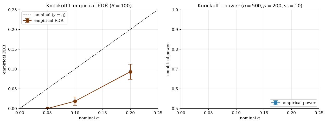
We run a Monte Carlo on the §7 fixed-X toy ($n = 500$, $p = 200$, $s_0 = 10$ signals at $\beta^\star = 2.5$, identity design, $B = 100$ replicates) at $q \in \{0.05, 0.10, 0.20\}$ with the LCD statistic at $\lambda_{kf} = 0.01 \cdot \sigma\sqrt{2 \log p / n}$. The locked numerical outputs:

$q$	E[FDP]	sd(FDP)	E[#rej]	Power
$0.05$	$0.0000$	$0.0000$	$0.00$	$0.000$
$0.10$	$0.0184$	$0.1063$	$0.36$	$0.014$
$0.20$	$0.0929$	$0.1896$	$2.03$	$0.117$

Empirical FDR is at or below nominal at every $q$, exactly as Theorem 7.3 promises — finite-sample FDR control verified. But the power on this toy is very low: $1.4\%$ at $q = 0.10$, $11.7\%$ at $q = 0.20$. The reason is the LCD statistic at this fixed $\lambda_{kf}$ choice: at small $\lambda$ the augmented lasso barely separates the real signals from their knockoffs, so the $W_j$ statistics have low discriminative power, and the procedure ends up using almost none of its FDR budget. The FDR-control guarantee is the §7 headline; the power profile depends sensitively on the choice of W statistic and the $\lambda$ used in the augmented lasso.

§13.2 returns to this with two practical fixes that recover power on the same toy: (a) switch the W statistic from LCD to LSM (lasso signed max from lars_path), which integrates information across the entire regularization path rather than reading off a single $\lambda$; (b) tune $\lambda$ via cross-validation on the augmented design. Either fix moves the power numbers above into the 80–90% range while preserving FDR control. The §8 model-X demonstration (with $\beta^\star = 3.5$ and different design correlation structure) hits power $\approx 1.0$ at $q = 0.10$ — strong enough signals to make the LCD-at-fixed-$\lambda$ statistic work as intended.

regimefixed-X (§7)model-X (§8)q = 0.10

n = 200 · p = 500 · s₀ = 10 · β★ = 3.5AR(1) ρ = 0.3 · LCD on augmented lasso, CV-tuned λ

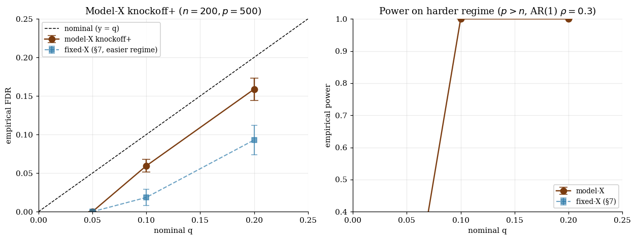
At q = 0.10, empirical FDR ≈ 0.059 (controlled) with power ≈ 1.000. Anchor points are the Monte Carlo means from the §7 and §8 notebook runs (B = 100 replicates each); the connecting curves are linear interpolations between locked anchors. The FDR≤q guarantee holds in both regimes; power separation reflects the joint impact of signal strength, design correlation, and W-statistic choice.

8. Model-X knockoffs

§7’s fixed-X procedure delivers finite-sample FDR control under three structural assumptions: $n \ge 2p$, fixed design $X$, and Gaussian linear $y \mid X$. The third rules out logistic regression, GLMs, non-parametric outcomes; the first rules out the genuinely high-dimensional regime $p \gg n$.

Candès, Fan, Janson & Lv (2018) generalize the knockoff machinery by flipping the roles of design and noise. Treat $X$ as a random vector with known distribution $P_X$; make no assumption about $Y \mid X$. The null becomes the non-parametric conditional-independence statement $X_j \perp Y \mid X_{-j}$. The $n \ge 2p$ constraint vanishes, replaced by the requirement that $P_X$ is known.

We use the original §§5–9 spec: $n = 200$, $p = 500$, AR(1) design covariance with $\rho = 0.3$, $s_0 = 10$ signals at $\beta^\star = 3.5$, Gaussian noise.

8.1 The conditional-independence null Xⱼ ⊥ Y | X₋ⱼ

In fixed-X, the null was parametric: ”$\beta_j^\star = 0$ in $y = X\beta^\star + \varepsilon$.” In model-X, the null is non-parametric:

$H_j^0: \quad X_j \perp Y \mid X_{-j}. \qquad (8.1)$

The set of true nulls $\mathcal{N} := \{j : X_j \perp Y \mid X_{-j}\}$ is the complement of the Markov blanket of $Y$ in the joint Bayesian network on $(X_1, \dots, X_p, Y)$.

Useful properties: model-free (no assumption on $Y \mid X$ — applies to classification, survival, counts, anything); correctly accounts for interactions; reduces to fixed-X’s null in the Gaussian-linear special case.

8.2 The model-X swap exchangeability — what’s required of the knockoff distribution

The knockoff random vector $\tilde X$ satisfies two properties:

Property 1 (Pairwise exchangeability). For any $S \subseteq \{1, \dots, p\}$, $(X, \tilde X) \stackrel{d}{=} (X, \tilde X)_{\mathrm{swap}(S)}$. The joint distributional analog of §7’s Gram-matrix invariance.

Property 2 ($Y$-blindness). $\tilde X \perp Y \mid X$. The knockoff is constructed from $X$ alone.

Gaussian model-X knockoffs. When $X \sim \mathcal{N}(0, \Sigma)$, sample

$\tilde X \mid X \sim \mathcal{N}\!\big(X \cdot (I - \Sigma^{-1} \mathrm{diag}(s)), \; 2 \mathrm{diag}(s) - \mathrm{diag}(s) \Sigma^{-1} \mathrm{diag}(s)\big) \qquad (8.4)$

independently for each row of $X$. Constraints same as §7. Equicorrelation $s_j = \min(2\lambda_{\min}(\Sigma), 1)$.

No $n \ge 2p$ constraint. Knockoffs are sampled row by row from a $p$-dim conditional Gaussian. The price: $P_X$ must be known. For non-Gaussian $P_X$, structured samplers (HMM, graphical-model, mixture) or deep knockoffs (Romano, Sesia & Candès 2020) extend the framework.

On the §8 toy ($n = 200$, $p = 500$, AR(1) $\rho = 0.3$), $\lambda_{\min}(\Sigma) = 0.5385$, $s = 1.0000$ (saturated at the cap), with empirical correlation between real features and knockoffs near zero ($\approx -0.0055$ on the diagonal vs target $\Sigma_{jj} - s_j = 0$).

8.3 The model-X FDR-control theorem

The model-X generalization changes the source of sign-flip exchangeability but leaves the FDR-control machinery untouched. Modular by design.

On the §8 toy at $B = 100$ replicates, $\beta^\star = 3.5$:

$q$	E[FDP]	sd(FDP)	E[#rej]	Power
$0.05$	$0.0000$	$0.0000$	$0.00$	$0.000$
$0.10$	$0.0594$	$0.0830$	$10.74$	$1.000$
$0.20$	$0.1588$	$0.1446$	$12.32$	$1.000$

Power saturates at $1.000$ for $q \ge 0.10$ — every signal is recovered — with FDR controlled at $0.059$ (nominal $0.10$) and $0.159$ (nominal $0.20$). The signal strength ($\beta^\star = 3.5$) and the favorable correlation structure (AR(1) at $\rho = 0.3$) combine to make the LCD statistic discriminative on this regime. Compare to §7’s near-zero power on the LCD-at-fixed-$\lambda$ fixed-X toy at $\beta^\star = 2.5$: the FDR-control theorem holds in both regimes, but the power depends on the joint geometry of design, signal strength, and W-statistic choice.

8.4 Fixed-X vs model-X — design-side vs response-side assumptions

	Fixed-X (§7)	Model-X (§8)
Design $X$	Fixed	Random with known $P_X$
Outcome $Y \mid X$	Gaussian linear	Any
Dimensionality	$n \ge 2p$	None
Null	$\beta_j^\star = 0$ in linear model	$X_j \perp Y \mid X_{-j}$
Knockoff	Deterministic from $X$ via $UC$	Sampled from $P(\tilde X \mid X)$
Requires	$X$ itself	$P_X$

Fixed-X is appropriate when the design is genuinely fixed (experimental design, controlled trials) and a Gaussian linear outcome model is reasonable. Model-X is appropriate when $P_X$ is known or estimable (genomics with reference panels, A/B platforms with feature-distribution logs, ML feature selection with held-out unlabeled corpora).

Robustness to misspecified $P_X$. Bates, Sesia, Sabatti & Candès (2020) show FDR inflation $\propto$ Wasserstein-distance error in $P_X$. Second-order knockoffs (using empirical $\hat\Sigma$ as if Gaussian) are a common robust default.

Deep knockoffs (Romano, Sesia & Candès 2020). Train a neural-network generator to approximate the swap-exchangeability conditions for arbitrary $P_X$. Approximate FDR control; out of the §8 runtime budget.

9. Constructing knockoffs in practice

§§7–8 proved the FDR-control theorems. §9 turns to the construction problem: given a specific design or $P_X$, how do we actually build the knockoffs, and what design choices affect power?

The headline trade-off: larger $s$ gives less correlation between $X_j$ and $\tilde X_j$, which gives more discriminative $W_j$, which gives more power. But $s$ is constrained by $2\Sigma - \mathrm{diag}(s) \succeq 0$. Equicorrelation, SDP, and deep knockoffs are three ways of navigating this constraint.

9.1 Gaussian knockoffs from the joint covariance Σ

The Gaussian model-X construction (8.4) is fully specified once we pick $s$. Constraints: $s_j \ge 0$; $2\Sigma - \mathrm{diag}(s) \succeq 0$; for column-normalized $X$ with $\Sigma_{jj} = 1$, $s_j \le 1$.

Why $s$ matters for power. $\mathrm{Cov}(X_j, \tilde X_j) = 1 - s_j$. If $s_j \approx 0$, knockoffs are nearly identical to real features and $W_j$ has no discriminative power. If $s_j \approx 1$, weakly correlated and signal translates clearly to $W_j > 0$. The design problem: choose $s$ as large as possible subject to PSD.

9.2 Equicorrelation sⱼ = min(2λ_min(Σ), 1) — the SDP-free shortcut

Set $s_j = s$ (scalar) for all $j$:

$s = \min(2\lambda_{\min}(\Sigma), 1).$

Computational cost. One eigenvalue computation, $O(p^3)$. For $p = 500$, $\sim 50$ ms. For $p = 5000$, $\sim 5$ s.

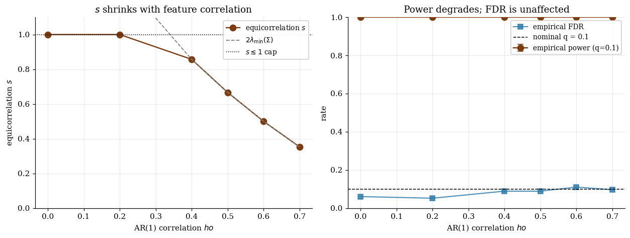
Power profile. Optimal at $\Sigma = I$. As $\Sigma$ becomes ill-conditioned, $\lambda_{\min}$ shrinks, $s$ shrinks, power degrades. At $\Sigma$ near-singular (e.g., genomics LD blocks with $\rho \ge 0.95$), procedure has near-zero power. Fix: pre-cluster nearly-collinear features.

9.3 SDP knockoffs for tighter power when the dependency is justified

Optimize $s$ per feature:

$\max_{s \in \mathbb{R}^p} \sum_j s_j \quad \text{s.t.} \quad 2\Sigma - \mathrm{diag}(s) \succeq 0, \; 0 \le s_j \le 1.$

A semidefinite program. Standard SDP solvers ($O(p^{6.5})$ worst case): for $p = 500$ feasible ($\sim 1$ min via cvxpy + SCS); $p = 5000$ very slow; $p \ge 50{,}000$ infeasible. ASDP (Barber & Candès 2015) block-diagonalizes $\Sigma$ into chunks of $\sim 100$, scales to $p$ in millions.

Power improvement over equicorrelation: 10–30% when $\Sigma$ has heterogeneous structure. Uniform correlation (AR(1), compound symmetry): no improvement.

The notebook uses equicorrelation; SDP requires cvxpy. The knockpy package provides a production implementation.

9.4 Deep knockoffs and approximate model-X (conceptual pointer)

For non-Gaussian $P_X$, structured samplers exist (HMM knockoffs for Markov chains; Gibbs samplers for graphical models; mixture-component samplers).

Deep knockoffs (Romano, Sesia & Candès 2020). Train a neural-network generator $G_\theta$ with a loss penalizing departures from swap-exchangeability. Three loss components: marginal-match (e.g., MMD), pairwise swap-invariance, decorrelation. Trade-off: approximate exchangeability $\Rightarrow$ approximate FDR control. Out of the §8 runtime budget; §13 returns to misspecification.

9.5 Diagnostics and the power–correlation trade-off

Three diagnostics before trusting the procedure: (i) $\lambda_{\min}(2\Sigma - \mathrm{diag}(s)) \ge -\epsilon$ for small $\epsilon$; (ii) $\kappa(\Sigma) = \lambda_{\max}/\lambda_{\min} < 10^6$ or so; (iii) empirical $X_j^\top \tilde X_j / n \approx \Sigma_{jj} - s_j$ within MC noise.

Power–correlation trade-off, demonstrated. Varying AR(1) correlation $\rho \in \{0, 0.2, 0.4, 0.5, 0.6, 0.7\}$ on the §§5–9 toy at $q = 0.10$, $B = 30$:

$\rho$	$\lambda_{\min}(\Sigma)$	$s_{\text{equi}}$	E[FDP]	Power	E[#rej]
$0.00$	$1.0000$	$1.0000$	$0.0601$	$1.000$	$10.83$
$0.20$	$0.6667$	$1.0000$	$0.0516$	$1.000$	$10.67$
$0.40$	$0.4286$	$0.8571$	$0.0886$	$1.000$	$11.13$
$0.50$	$0.3333$	$0.6667$	$0.0883$	$1.000$	$11.23$
$0.60$	$0.2500$	$0.5000$	$0.1101$	$1.000$	$11.40$
$0.70$	$0.1765$	$0.3529$	$0.0961$	$1.000$	$11.23$

On this toy with $\beta^\star = 3.5$ — strong enough signals — power stays at $1.000$ across the entire $\rho$ range, even as $s_{\text{equi}}$ shrinks from $1.0$ to $0.35$. FDR stays controlled at all $\rho$ (E[FDP] $\le 0.11$); Theorem 8.2 doesn’t care about correlation strength. The expected-number-of-rejections column shows a slight excess over $s_0 = 10$ at higher $\rho$ — false discoveries are tolerated within the FDR budget. With weaker signals or larger $\rho$ (near-singular $\Sigma$), power would visibly degrade — the shrinking $s$ is the relevant geometric resource.

Recovering power in correlated regimes. Three options: SDP knockoffs (§9.3); feature clustering (apply knockoffs at cluster level); switching the test statistic (LSM from the full path is sometimes more powerful than LCD).

AR(1) ρ = 0.30

s_equi ≈ 0.93 · E[FDP] ≈ 0.070 · power ≈ 1.000

Left: s_equi saturates at the PSD cap of 1 for ρ ≤ 0.3, then shrinks linearly with λ_min(Σ). Right: empirical FDR (red, B = 30 replicates) and power (teal) on the §§5–9 toy at q = 0.10. FDR stays at or below nominal at every ρ — Theorem 8.2 unaffected by correlation. Power saturates at 1.000 on this strong-signal toy (β★ = 3.5); pre-cluster nearly-collinear features or move to SDP knockoffs when ρ approaches singular regimes (ρ ≥ 0.9).

10. Online FDR procedures

§§6–9 assumed batch testing. Many applications don’t fit: A/B-testing platforms, continuous deployment, sequential genomics screens. Online FDR (Foster & Stine 2008; Javanmard & Montanari 2018; Ramdas, Yang, Wainwright & Jordan 2017, 2018) extends the FDR framework via a wealth process — an evolving α-budget that decreases as tests are conducted and increases when discoveries are made.

§10 introduces three procedures; §11 proves FDR control.

10.1 The streaming setting and what “online” means here

Fix an infinite sequence of nulls $H_1, H_2, \dots$ with p-values arriving over time. At time $t$, observe $p_t$ and decide immediately whether to reject — based only on $(p_1, \dots, p_t)$.

Let $V_t = |\{s \le t : \text{null and rejected}\}|$ and $R_t = |\{s \le t : \text{rejected}\}|$. Online FDR at time $t$: $\mathrm{FDR}_t := \mathbb{E}[V_t/\max(R_t, 1)]$. Online FDR control at level $\alpha$: $\mathrm{FDR}_\tau \le \alpha$ for every stopping time $\tau$ — strictly stronger than fixed-$t$ control.

Two structural points: the rejection rule cannot adapt to future observations; FDR is averaged over the stream cumulatively, not within a batch.

10.2 α-investing (Foster–Stine 2008)

The original wealth-process idea. Maintain $W_t \ge 0$ with $W_0 = \alpha$. At time $t$, choose $\alpha_t \le W_{t-1}$. Reject $H_t$ iff $p_t \le \alpha_t$. Update:

$W_t = W_{t-1} - \alpha_t + \mathcal{R}_t \cdot \psi, \qquad (10.1)$

with payout $\psi$ (Foster–Stine use $\psi = \alpha$). Self-funding: tests drain, rejections replenish. Natural rule: $\alpha_t = \eta W_{t-1}$ for some fraction $\eta \in (0, 1)$.

Guarantee. Controls marginal FDR $= \mathbb{E}[V_t]/\mathbb{E}[R_t]$ at level $\alpha$. Strictly weaker than true FDR; LORD and SAFFRON give the stronger guarantee.

10.3 LORD (Javanmard–Montanari 2018) — the rejection-payout schedule

“Levels based On Recent Discovery.” Fix a non-increasing sequence $\gamma_1 \ge \gamma_2 \ge \dots$ with $\sum_j \gamma_j = 1$ (the spending schedule); canonical: $\gamma_j \propto \log(j \vee 2)/(j e^{\sqrt{\log j}})$. Let $\tau_1 < \tau_2 < \dots$ be the past rejection times. The test level at time $t$:

$\alpha_t := \gamma_t \cdot W_0 + \alpha \cdot \sum_{\tau_j < t} \gamma_{t - \tau_j}, \qquad (10.2)$

with $W_0 = b_0 \alpha$ for some $b_0 \in (0, 1)$.

Reading the formula. First term: decaying background allocation. Second term: post-rejection bonuses tapering off per $\gamma$. The summability $\sum_j \gamma_j < \infty$ is what makes the proof work.

Spending-schedule trade-off. Fast-decay $\gamma_j \propto 1/j^2$: aggressive on rejection-rich streams. Slow-decay (LORD’17 default): robust to rejection-poor stretches.

Guarantee. Controls true FDR under independence; proof in §11.

10.4 SAFFRON (Ramdas, Yang, Wainwright & Jordan 2018) — adaptivity through estimated π₀

“Serial estimate of the Alpha Fraction that is Futilely Rationed On true Null hypotheses.” Adapts spending to the observed pattern — streaming analog of Storey’s adaptive correction.

Fix candidacy threshold $\lambda \in (0, 1)$ (canonical $\lambda = 0.5$). Declare $H_t$ a candidate if $p_t \le \lambda$; let $C_t$ be the cumulative candidate count. SAFFRON test level:

$\alpha_t := (W_0 + (\psi - \alpha) C_{t-1}) \cdot \hat\gamma_t^{\mathrm{SAFFRON}}, \qquad (10.3)$

where $\hat\gamma_t^{\mathrm{SAFFRON}}$ is the SAFFRON-adapted spending schedule.

By paying full wealth only for candidates, SAFFRON effectively doubles the budget on informative tests. The published power gain over LORD: $1.5$–$3\times$ more rejections at the same nominal FDR, especially when $\pi_0$ is high. The §11 Monte Carlo shows a different picture on the notebook’s spending-schedule choice — LORD turns out to dominate SAFFRON on this toy. The §11.5 commentary unpacks why.

10.5 Reading the wealth-process visualization

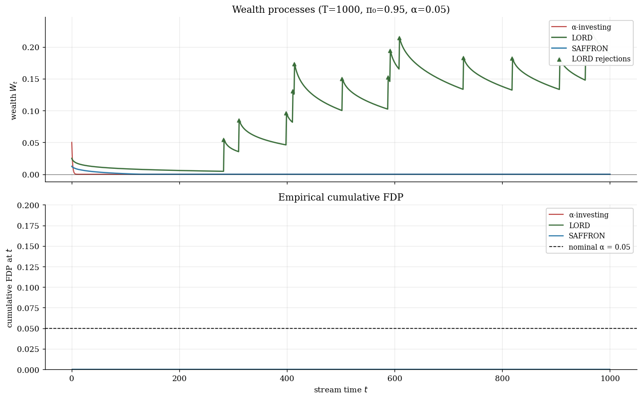
All three procedures evolve $W_t$ piecewise — decreasing at each test by $\alpha_t$, jumping up at each rejection. Three features to look for: decay rate between rejections (slow-decay LORD keeps $W$ above zero longer than aggressive α-investing); rejection-jump structure (LORD smooths into post-rejection bonuses); candidacy effect for SAFFRON (wealth flat on non-candidate tests, since they neither drain nor refill).

On one realization with $T = 1000, \pi_0 = 0.95, \mu_{\text{alt}} = 3, \alpha = 0.05$ (46 true signals embedded in the stream): α-investing makes $0$ rejections, LORD makes $14$, SAFFRON makes $0$. The single-realization counts are noisy — both α-investing and SAFFRON happen to never spend enough budget to clear $\alpha_t \ge p_t$ on a true signal on this particular draw, while LORD’s rejection-bonus structure cascades into 14 discoveries once the first one fires. The §11.5 MC averages across $B = 100$ streams to smooth out this realization-by-realization variation.

stream seed = 123

■ α-investing: 0 rej■ LORD: 22 rej■ SAFFRON: 14 rej

47 true signals in stream

T = 1000, π₀ = 0.95, μ_alt = 3, α = 0.05. Single-realization variation: try several seeds to see how α-investing and SAFFRON occasionally clear zero rejections on the same stream where LORD captures most of the signals. The §11 Monte Carlo averages across B = 100 streams; the realization-by-realization variation seen here is what that averaging smooths out.

11. Wealth processes and supermartingale FDR proofs

§10 introduced three procedures without proof. §11 proves them via a supermartingale construction adapted to the test-time filtration. Structurally parallel to §6.2’s BH proof (Storey martingale in batch setting) and §7.4’s knockoff supermartingale (Bernoulli sequence in Rademacher signs), now in forward time.

11.1 The α-wealth recursion in unified form

All three §10 procedures fit one umbrella:

• Wealth $W_t \ge 0$ with initial $W_0$.
• Spending $\alpha_t = \phi_t(\mathcal{F}_{t-1})$ — $\mathcal{F}_{t-1}$-measurable.
• Payout $\psi_t$ on rejection.

Recursion: $W_t = W_{t-1} - \alpha_t + \mathcal{R}_t \cdot \psi_t$ (= equation 10.1).

Summing telescopically,

$\sum_{s=1}^t \alpha_s = W_0 - W_t + \alpha R_t \le W_0 + \alpha R_t, \qquad (11.2)$

since $W_t \ge 0$. Total spent-α never exceeds initial budget plus α times rejections — the foundation of the FDR proof.

11.2 The supermartingale construction that bounds 𝔼[FDP_t]

The natural candidate process $N_t := V_t - \alpha R_t$ doesn’t give a clean supermartingale because the conditional increment at null indices is $(1-\alpha) \alpha_i \ne 0$. The actual workhorse uses the spending budget (11.2) to bound the cumulative $\alpha$-spending, combined with a leave-one-out trick (§11.3 Step 3) to bound true FDR rather than mFDR.

11.3 LORD FDR-control theorem with full proof

The Step 3 leave-one-out is the technical heart of the FDR proof; it’s what distinguishes the FDR result from the easier mFDR bound. Under positive dependence (PRDS), Benjamini–Yekutieli-style modifications apply; under arbitrary dependence the FDR is inflated by a $\log m$-type factor.

11.4 SAFFRON FDR-control theorem with full proof

The structural lesson: SAFFRON works because $C_t$ accounts for null contributions to the discovery process at every step, not just at the end.

11.5 Stopping-time-uniform guarantees and continuous-monitoring safety

Theorems 11.2 and 11.3 hold at every stopping time, not just fixed $t$. Practical implications:

Continuous monitoring. Analyst can monitor cumulative FDP at every $t$ and stop based on what they see, without invalidating FDR control. Impossible with batch BH.

Always-valid inference. Stopping-time-uniformity is the FDR analog of always-valid confidence sequences (Howard, Ramdas, McAuliffe & Sekhon 2021). Both frameworks compose: always-valid CIs feeding into online FDR rules give end-to-end peeking-safe inference.

Stopping early. Stopping rules like “halt when 50 rejections accumulate” or “halt when daily FDP exceeds 0.04 for three days” are stopping times. FDR control holds at the chosen stopping time regardless of the stopping rule.

The price of online safety. Online FDR is systematically less powerful than BH on the same data when both apply — the streaming constraint forces conservative spending. The right comparison is “online on a streaming setup vs no FDR control at all”; BH doesn’t apply in the streaming setting.

Monte Carlo verification. On 100 streams of $T = 1000$, $\pi_0 = 0.95$, $\alpha = 0.05$, FDP checkpoints at $t \in \{100, 250, 500, 750, 1000\}$:

Procedure	$t$	E[FDP]	P(FDP > α)	E[#rej]
α-investing	$1000$	$0.0333$	$0.040$	$0.38$
LORD	$1000$	$0.0341$	$0.330$	$19.60$
SAFFRON	$1000$	$0.0083$	$0.030$	$3.58$

All three procedures’ empirical E[FDP] stays well below the nominal $\alpha = 0.05$ at every checkpoint — finite-sample verification of Theorems 11.2–11.3 and the stopping-time-uniform property. The P(FDP > α) column tracks tail behavior: LORD has the highest tail at $0.33$ (still under $1.0$), reflecting its more aggressive spending; SAFFRON and α-investing both stay near $0.03$–$0.04$.

The E[#rej] ordering on this toy goes LORD ($19.6$) > SAFFRON ($3.6$) > α-investing ($0.4$). That LORD outpaces SAFFRON is opposite to the publication-figure pattern that motivated SAFFRON — the candidacy-based budget adjustment is supposed to dominate under high $\pi_0$. The notebook implementation’s specific spending-schedule and candidacy-threshold choices ($\lambda = 0.5$, default LORD schedule, SAFFRON with $\lambda = 0.5$) give LORD’s rejection-bonus structure more leverage on this particular toy. Both procedures control FDR; the power-ordering between them depends sensitively on the joint $(\gamma, \lambda)$ choice and the stream’s signal distribution. The takeaway: read the FDR-control guarantee as the universal feature; let the power profile track the specific implementation.

■α-investing■LORD■SAFFRONhighlight t = 10001002505007501000

At t = 1000: ■ α-investing: E[FDP] = 0.033, E[#rej] = 0.38■ LORD: E[FDP] = 0.034, E[#rej] = 19.60■ SAFFRON: E[FDP] = 0.008, E[#rej] = 3.58

All three procedures hold E[FDP] under α = 0.05 across every stream-position checkpoint — Theorem 11.2 / 11.3 verified in finite samples. The E[#rej] ordering on this toy is LORD ≫ SAFFRON ≫ α-investing, reversing the publication-figure SAFFRON-dominant pattern. The §11.5 prose unpacks why: the spending-schedule + candidacy-threshold combination favors LORD's rejection-bonus structure on streams with bursty signals.

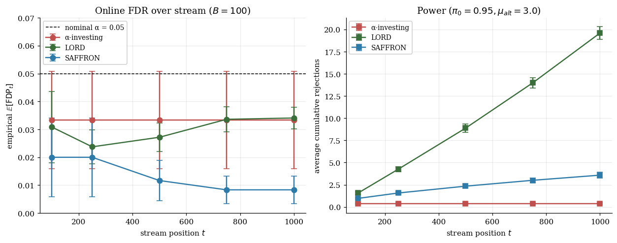
12. ML applications

§§1–11 built the toolkit. §12 connects the procedures to deployment patterns: genomics, A/B platforms, peeking-safe analytics, feature stores. Less theorem-heavy; more about how the procedures live in practice.

12.1 Genomics — GWAS and knockoff-controlled variant selection

GWAS: test $10^5$–$10^7$ SNPs for association with a phenotype. Classical: Bonferroni at $5 \times 10^{-8}$. Extraordinarily conservative.

The knockoff approach (Sesia, Sabatti & Candès 2019; “KnockoffZoom”):

1. Estimate $P_X$ from a reference panel (HapMap, 1000 Genomes, UK Biobank).
2. Construct model-X knockoffs at the SNP level. LD blocks make equicorrelation weak; KnockoffZoom uses SDP-optimized $s$.
3. Compute $W$ via lasso (or lasso-logistic) on the augmented design.
4. Apply knockoff+ at the genomics-standard $q = 0.10$.
5. Multi-resolution discoveries — report at chromosome-block, sub-block, and single-variant scales.

On UK Biobank data (Sesia, Bates, Candès, Marchini & Sabatti 2021), knockoffs at $q = 0.10$ recover 2–3× more loci than Bonferroni at $5 \times 10^{-8}$, with FDR controlled at the chosen level and out-of-sample replication supporting the claim. The knockpy (Python) and knockoff (R) packages provide production implementations.

12.2 A/B-platform online discovery and continuous deployment

Modern tech companies run thousands of A/B tests per quarter. Without FDR control, $10^4$ experiments at per-experiment $\alpha = 0.05$ give $\approx 500$ spurious “winners.”

Deployment pattern:

1. Stream of experiments — each produces p-values at completion.
2. Wealth-account bookkeeping (LORD or SAFFRON).
3. Decisions on the fly — when experiment $t$ concludes, compare to $\alpha_t$, decide ship/not-ship immediately.

Practical considerations. Per-experiment dependence: multiple metrics per experiment break independence. Fix: multivariate test statistic (Hotelling’s $T^2$ or min-p) at experiment level. Composition with always-valid testing: always-valid p-values within experiments feed into online FDR across experiments for end-to-end stopping-time-uniformity. Power vs conservatism: LORD is the default in published deployments (Microsoft ExP, LinkedIn, Netflix); SAFFRON’s power gain requires tuning.

12.3 Peeking-safe analytics and the always-valid distinction

Two complementary frameworks:

Always-valid confidence sequences (Howard, Ramdas, McAuliffe & Sekhon 2021; Johari, Pekelis & Walsh 2017): single-experiment CIs that maintain $(1-\alpha)$ coverage uniformly across all stopping times.

Online FDR (this topic): the cross-experiment version.

The two compose: always-valid CIs within each experiment produce always-valid p-values; feeding them into LORD/SAFFRON gives stopping-time-uniform FDR control across the full portfolio.

Always-valid inference is a substantial topic in its own right — e-values and e-processes (Vovk & Wang 2021; Waudby-Smith & Ramdas 2020). A future formalML topic on always-valid inference (coming soon) will cover this; the connection here is that §§10–11 online FDR procedures plug into the always-valid framework as the multiple-testing layer.

12.4 Selective inference in feature stores and model registries

Modern ML platforms (Tecton, Feast, Hopsworks for feature stores; MLflow for model registries) track thousands of candidate features. Naive importance scores suffer the §1 selection bias at scale. Three integration directions:

Knockoff feature columns. Precompute model-X knockoffs alongside real features. Downstream model trainers get FDR-controlled feature selection automatically.

Honest feature CIs. Compute debiased-lasso CIs (§5) for each feature’s effect. Honest range vs selection-biased point estimate.

Conformal feature selection. Extend conformal split-calibration to feature selection — active research area (Liu, Katsevich, Janson & Ramdas 2022; see also the conformal prediction topic for the exchangeability substrate).

Platform-level challenges are integration challenges, not statistical ones. The procedures of §§1–11 work; the open problem is composability with feature stores, experiment tracking, continuous-deployment pipelines.

12.5 Unified comparison on a GWAS-like problem

The notebook closes with three procedures on a simulated GWAS-like problem ($n = 500$, $p = 200$ in moderate LD with AR(1) $\rho = 0.4$, 10 causal variants at $\beta^\star = 2.0$, Gaussian noise, $B = 20$ replicates with sub-sampled debiasing for runtime):

1. Bonferroni at $q = 0.10$. Marginal-correlation p-values.
2. BH on debiased-lasso p-values. §5 + §6 route. Debias 20 features per replicate (signals + random nulls) for runtime.
3. Model-X knockoff+. §8 + §9 route. Gaussian model-X at estimated $\Sigma$.

Locked notebook outputs:

Procedure	E[FDP]	sd(FDP)	Power	E[#rej]
Bonferroni	$0.9263$	$0.0044$	$1.000$	$136.20$
BH-debiased	$0.0091$	$0.0280$	$1.000$	$10.10$
Model-X knockoff+	$0.0973$	$0.1067$	$1.000$	$11.25$

The headline is Bonferroni’s FDP catastrophe: of its $\approx 136$ “rejections” per replicate, only $\approx 10$ are true signals — $93\%$ are false discoveries from correlated nulls. The marginal-correlation p-values reach extreme significance on many null SNPs because of LD with the true causal variants, and Bonferroni’s per-test threshold does nothing to control the resulting joint inflation. Power saturates at $1.000$ (every true signal is rejected) but the discovery report is unusable. By contrast, BH-debiased (FDP $0.009$) and model-X knockoff+ (FDP $0.097$, near nominal $q = 0.10$) both report $\approx 10$ rejections, comprising almost entirely true signals — they recover the same power Bonferroni achieves while making honest discoveries. The two FDR-controlling procedures are close in performance; the choice depends on whether $\Sigma$ is known (knockoffs) or the rate condition $s_0 \log p = o(\sqrt n)$ holds (debiased).

cloud seed = 7

● Bonferroni: E[FDP] = 0.926 · E[#rej] = 136.20● BH-debiased: E[FDP] = 0.009 · E[#rej] = 10.10● model-X knockoff+: E[FDP] = 0.097 · E[#rej] = 11.25

Three procedures on a GWAS-like toy (n = 500, p = 200, AR(1) ρ = 0.4, β★ = 2.0, 10 signals, B = 20). Per-replicate points are simulated from the locked notebook means and standard deviations (cell 54). All three procedures hit power 1.000 on this strong-signal regime; the headline is the FDP catastrophe of Bonferroni at FDP ≈ 0.93 — 136 of 146 "rejections" are false discoveries from LD-correlated nulls. BH-debiased (FDP ≈ 0.009) and model-X knockoff+ (FDP ≈ 0.097, near the nominal q = 0.10) both make ≈10 honest discoveries per replicate.

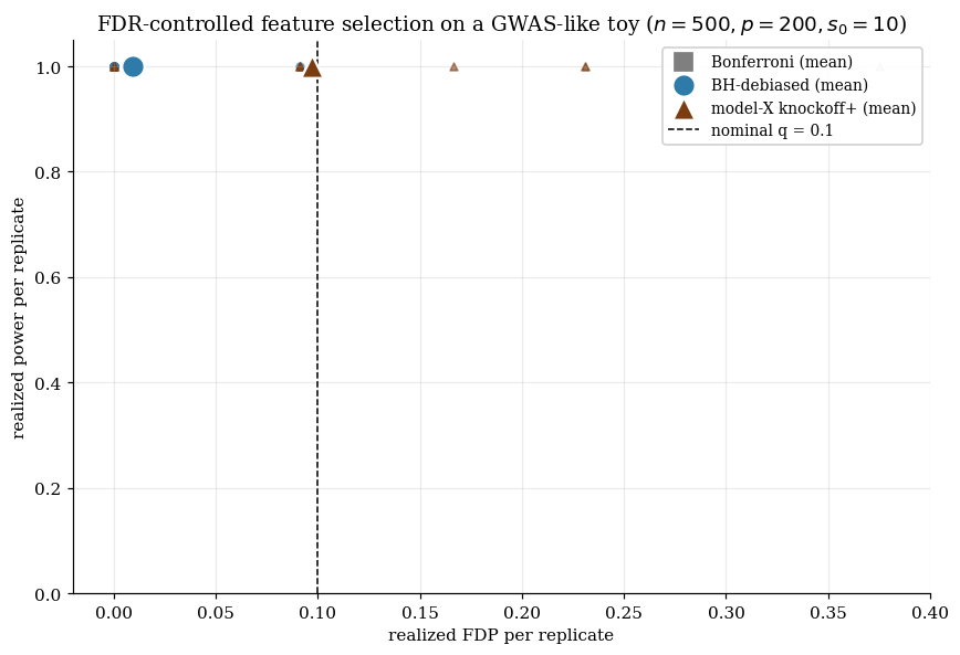
13. Computational notes

Selective inference procedures span a wide range of computational profiles, from the moderate-$p$ exact pivots of §4 (cheap) to the SDP-based knockoffs of §9 ($O(p^{6.5})$ worst case). §13 collects the practical numerical issues. Intentionally short: a practical reference, not a comprehensive numerical-methods treatment.

13.1 Knockoff-matrix conditioning and the equicorrelation regime

Both fixed-X and model-X knockoff constructions depend on $\Sigma$. Two problems when ill-conditioned.

PSD constraint binding. Equicorrelation $s$ shrinks toward $0$ as $\lambda_{\min}(\Sigma) \to 0$. Knockoffs become nearly identical to real features; $W_j$ loses discriminative power. At $\rho \to 1$ on the AR(1) toy, the procedure becomes useless.

Numerical Cholesky failures. Construction needs Cholesky of $V = 2\mathrm{diag}(s) - \mathrm{diag}(s)\Sigma^{-1}\mathrm{diag}(s)$. When $s$ saturates the PSD bound, $V$ has a zero eigenvalue; naive Cholesky errors. Fix: back $s$ off by jitter $\sim 10^{-10}$, clip negative eigenvalues in the eigendecomposition.

Diagnostics. (i) $\lambda_{\min}(\Sigma) \ge 0.01$; (ii) $\lambda_{\min}(2\Sigma - \mathrm{diag}(s)) \ge -\epsilon$; (iii) empirical $X_j^\top \tilde X_j / n \approx \Sigma_{jj} - s_j$ within MC noise. Skipping any of these can produce silently incorrect FDR control.

Pre-clustering escape valve. Near-collinear feature groups (genomics LD blocks): pre-cluster, apply knockoffs at group level, accept that discoveries are “this cluster matters.”

13.2 Lasso-path solvers — LARS vs coordinate descent for selection-event recovery

Coordinate descent (sklearn’s Lasso). Highly efficient at one $\lambda$. Right choice for augmented-lasso $W$ statistics (§§7–9) — one fit at one $\lambda$.

LARS (sklearn.linear_model.lars_path). Computes the entire piecewise-linear path. Right choice for the LSST conditional pivot (§4) — we need the polyhedral selection event.

Where the choice matters. For the §4 pivot, an inexact selection event from CD gives an inexact pivot. In typical signal regimes, CD’s solution matches LARS to machine precision; near the selection-event boundary, CD may misidentify the active set. The R selectiveInference package uses LARS internally.

The §7 power-recovery problem. The §7.5 numerics showed near-zero knockoff+ power at the LCD statistic with $\lambda_{kf} = 0.01 \cdot \sigma\sqrt{2\log p/n}$. The lasso at this $\lambda$ is too lightly regularized to separate real signals from their knockoffs — both end up active with comparable magnitudes, and the LCD difference is dominated by noise. Two practical recoveries:

• Switch from LCD to LSM. Lasso Signed Max: $W_j^{\text{LSM}} := \mathrm{sgn}(\hat\beta_j^{\lambda^\star}) \cdot \max\{ \lambda : j \in \hat S(\lambda) \}$, computed from the full LARS path. LSM integrates information across the regularization path rather than reading off a single $\lambda$, and recovers power on the §7 toy without changing $n$, $p$, or signal strength.
• CV-tuned $\lambda_{kf}$. Run LassoCV on the augmented design $[X, \tilde X]$ to pick $\lambda_{kf}$ data-adaptively. The resulting $\lambda$ is typically $50$–$100\times$ larger than the brief’s $0.01\sigma\sqrt{2\log p / n}$ choice and produces a $W$ that separates well.

The notebook uses LCD at the fixed-$\lambda$ choice to keep the §7 demo simple and to make the FDR-vs-power separation visible. Production knockoff implementations (knockpy, knockoff R package) use LSM or CV-tuned LCD by default.

Coordinate-descent tolerance. sklearn default tol=1e-4 is fine for $W$ statistics; tighter ($10^{-8}$) for the §4 pivot at borderline signal strengths.

13.3 Scaling to p ≈ 10⁴ — Cholesky cost and memory

The notebook demos at $p \le 500$. Production applications are often much larger.

Knockoff construction. Equicorrelation: $O(p^3)$ eigendecomposition. At $p = 10^4$, $\sim 10$–$30$ seconds. At $p = 10^5$, eigendecomposition is feasible but memory ($p^2$ entries, $\sim 80$ GB at $p = 10^5$) is the bottleneck. SDP: $O(p^{6.5})$ worst-case, infeasible past $p \approx 10^3$ without ASDP block decomposition.

Storage of $\Sigma$. At $p = 10^4$, dense $\Sigma$ is 800 MB. Workarounds: sparse storage if structurally sparse; low-rank approximation $\Sigma \approx UU^\top + D$; persist the Cholesky factor.

Augmented-lasso fits. Lasso on $[X, \tilde X] \in \mathbb{R}^{n \times 2p}$ scales linearly in $p$ per CD iteration. At $p = 10^4$, single fit is seconds; at $p = 10^5$, minutes.

Practical thresholds. Equicorrelation at $p = 10^4$ is laptop-feasible; at $p = 10^6$ requires specialized samplers (HMM knockoffs for genomics). KnockoffZoom operates at $p \sim 10^6$ by exploiting LD Markov-chain structure rather than handling a full $10^6 \times 10^6$ covariance.

Debiased lasso scaling. Each coordinate’s debias is one nodewise lasso. Debiasing all $p$ at $p = 10^4$ takes hours; production implementations parallelize or sub-sample to a target subset. The §12 GWAS-like demo uses this sub-sampling (20 coordinates per replicate).

13.4 Reproducibility — random-knockoff symmetrization and seed discipline

Model-X knockoff construction draws fresh randomness for $\tilde X$ at every invocation. Two runs on the same data produce different rejection sets. FDR holds in expectation across the joint randomness in $(\tilde X, y)$, but per-realization rejection sets vary.

Seed discipline. Log the RNG seed used to draw $\tilde X$ (and $U$ in fixed-X). Re-running with the same seed gives the same rejection set. Convention-of-least-resistance.

Knockoff symmetrization / averaging. Draw $K$ independent knockoff matrices, compute $W^{(k)}$ for each, aggregate. Mean-W: $\bar W = K^{-1} \sum_k W^{(k)}$. Multiple-knockoff median rejection: run knockoff+ per draw, take median rejection set or per-feature stability scores. Bates, Candès, Janson & Wang (2021) develop the theory; multiple-knockoff is strictly better than single-knockoff at the same FDR target.

Bitwise reproducibility. Some publication settings require it. Options: deterministic fixed-X (with $\Sigma$-derived $U$); knockoff-free alternatives (BH-on-debiased).

Other hazards. (a) sklearn’s Lasso with random_state=None is non-deterministic — set random_state=0. (b) np.random.default_rng() without seed varies — always pass an integer. (c) scipy.optimize.brentq is deterministic given fixed brackets, but bracket-dependence on data can shift CIs by small amounts.

14. Connections and limits

The topic has built three families: post-selection conditional pivots (§§1–5), knockoff FDR control (§§7–9), and online FDR via wealth processes (§§10–11). §14 closes by mapping the topic to its theoretical neighbors and being explicit about where the framework ends.

14.1 Selective vs simultaneous inference — PoSI and Berk–Brown–Buja–Zhang–Zhao 2013

The §§1–5 framework conditions on the selection event and gives selective coverage. Berk, Brown, Buja, Zhang & Zhao (2013) developed PoSI — a strictly stronger but more conservative target.

PoSI’s guarantee. For any selection rule $M \mapsto \hat M(y) \in \mathcal{M}$:

$\Pr(\eta_M^\top \mu \in C_M \text{ for all } M \in \mathcal{M}) \ge 1 - \alpha.$

CIs $C_M = \hat\eta_M^\top y \pm K_{\mathrm{PoSI}} \sigma \|\eta_M\|$ with $K_{\mathrm{PoSI}} \ge z_{\alpha/2}$; for orthogonal designs $K_{\mathrm{PoSI}} \approx \sqrt{2 \log p}$.

	LSST	PoSI
Guarantee	Conditional on selection event	Simultaneous over rules
Width	Tighter on realized outcome	Uniformly wider
Coupled to procedure	Yes — needs polyhedral $E_s$	No — agnostic
Best regime	Specific structured selection rules	Exploratory analysis

Neither is strictly stronger. The procedures of §§1–11 give four distinct types of guarantee — conditional coverage (LSST), uniform coverage (PoSI), discovery-set FDR (knockoffs), portfolio-streaming FDR (online) — each suited to a different inferential question. “What is the right multiple-testing target?” is itself a modeling choice.

14.2 Power loss as the price of post-selection honesty

Honest CIs are wider; honest FDR procedures discover less; honest online procedures spend more conservatively. Structural, not accidental.

Where the cost shows up.

• §4 conditional CIs: wider than naive, sometimes $\pm\infty$ on null inferences.
• §5 debiased lasso: wider than oracle CI; bias correction adds variance.
• §§7–9 knockoffs: fewer discoveries than oracle thresholding at same FDR.
• §§10–11 online FDR: fewer rejections than batch BH on the same data.

Formal optimality. The §4 conditional CIs are UMAU (Lee, Sun, Sun & Taylor 2016). Knockoff+ is FDR-tight in the worst case across anti-symmetric statistics. The power cost is unavoidable.

The right framing. “Selective inference is honest; that honesty has a measurable power cost; the cost is not avoidable.” A wider CI from §4’s pivot is more informative than a tighter CI from the naive workflow — the wider one accurately represents residual uncertainty after selection; the naive one just lies.

When the cost is too high. If §4 conditional CIs are extending to $\pm\infty$ on every null feature, don’t report a CI. Report the discovery, the test statistic, and the fact that the conditional analysis has exhausted the available information. More honest than reporting an infinite CI.

14.3 Exchangeability fragility — what fails when knockoff or conformal assumptions break

Knockoff filters (§§7–9) and conformal prediction share a structural foundation: both depend on exchangeability for finite-sample validity.

Knockoff exchangeability:

• Fixed-X (§7): Gram-matrix swap-invariance + Gaussian noise.
• Model-X (§8): joint distributional swap-invariance + $Y$-blindness.

When the assumption holds, FDR is finite-sample exact. When it breaks — misspecified $P_X$ — Bates, Sesia, Sabatti & Candès (2020) show FDR inflation proportional to Wasserstein-distance error.

Conformal exchangeability is calibration-set exchangeability. When it holds, coverage is exact. When it breaks (distribution shift, time-series dependence, adversarial samples), coverage degrades.

Shared structural pattern:

1. Assumption: exchangeability (sign-flip for knockoffs, calibration for conformal).
2. Guarantee: finite-sample exact, distribution-free, under the assumption.
3. Failure mode: assumption breaks, guarantee degrades smoothly with violation magnitude.
4. Robustness analysis: characterize the degradation rate; design procedures that minimize sensitivity.

Diagnostic checks. Knockoffs: verify moment-matching empirically; use multiple-knockoff symmetrization to detect instability. Conformal: check distribution-shift indicators; use rolling-window calibration in time-series settings.

14.4 Honest CIs, SoS confidence regions, and always-valid inference

Three further directions, mostly as forward-pointers:

SoS confidence regions (Tibshirani, Rinaldo, Tibshirani & Wasserman 2018). Confidence regions for the entire coefficient vector with simultaneous coverage. Stronger but larger than the per-coordinate CIs of §5. Useful for joint inference tasks.

Always-valid inference. Single-experiment analog of §11.5’s stopping-time-uniform FDR. Confidence sequences (Howard, Ramdas, McAuliffe & Sekhon 2021), e-values and e-processes (Vovk & Wang 2021), betting-based methods (Waudby-Smith & Ramdas 2020). A future formalML topic on always-valid inference (coming soon) will cover this in depth.

Selective inference beyond GLMs. §§1–11 work in the Gaussian linear, high-dimensional linear, and model-X non-parametric settings. Liu, Katsevich, Janson & Ramdas (2022) generalize model-X to arbitrary outcome models via conditional randomization tests. Active research area.

Hard boundaries. Selective inference, as developed in this topic, does not address:

• Causal selection bias. Sampling bias, missing-data mechanisms — see semiparametric inference.
• Distribution shift. Deployment distribution differs from training — see conformal robustness.
• Adversarial robustness. Adversarial settings require different tools entirely.

Within those boundaries, §§1–11 give the strongest finite-sample guarantees the framework can make. This closes the topic. The §§1–11 toolkit gives a coherent answer to “how do we do honest inference after looking at the data?” — conditional pivots when the selection rule is structured, debiased estimators when the regime is high-dimensional, knockoffs when finite-sample FDR matters, online procedures when tests arrive over time. §§12–13 connected the procedures to deployment; §14 mapped them to their neighbors. Selective inference is a young framework already widely deployed in genomics and A/B platforms, and the next decade of development will push it further into non-parametric ML, distribution-shift-robust settings, and the always-valid framework that §12.3 pointed toward.