Semiparametric Inference

§1. Motivation

Most of statistical learning theory treats either parametric models (a finite-dimensional parameter, classical asymptotic theory) or nonparametric models (an infinite-dimensional object, slower rates) as separate concerns. Semiparametric inference is what happens at the seam: we want $\sqrt n$-consistent, asymptotically normal estimates of a finite-dimensional functional — a treatment effect, a regression slope, a quantile shift — while letting the rest of the model be infinite-dimensional and estimated by whatever flexible learner we like. The puzzle is that finite-dimensional targets and infinite-dimensional nuisances usually move at different rates. Naively combining them costs us either bias (from plug-in estimation of the nuisance) or efficiency (from ignoring structure that’s actually there). The semiparametric framework explains exactly when and how the $\sqrt n$ rate survives, and gives a recipe — the efficient influence function — for building estimators that achieve it.

1.1 The semiparametric setup

Fix a model $\mathcal{M} = \{P_{\theta, \eta} : \theta \in \Theta,\ \eta \in \mathcal{H}\}$ where $\theta \in \mathbb{R}^k$ is the parameter of interest (the thing we want a confidence interval for) and $\eta$ is a nuisance living in some infinite-dimensional space $\mathcal{H}$ — a regression function, a density, a propensity score. Three running examples make the abstraction concrete.

Functional mean under missingness at random. We observe $O = (Y \cdot R,\ R,\ X)$ where $R \in \{0, 1\}$ indicates whether $Y$ is recorded. We want $\theta = \mathbb{E}[Y]$, with nuisances $\eta = (m, \pi)$ — the outcome regression $m(x) = \mathbb{E}[Y \mid X = x, R = 1]$ and the missingness propensity $\pi(x) = \Pr(R = 1 \mid X = x)$. We derive its efficient influence function from scratch in §3 and run a one-step estimator end-to-end in §5.

Average treatment effect under unconfoundedness. We observe $O = (Y, D, X)$ with $D \in \{0, 1\}$ a treatment indicator and $X$ pre-treatment covariates. We want $\theta = \mathbb{E}[Y(1) - Y(0)]$, with nuisances $\eta = (\mu_1, \mu_0, \pi)$ — the two conditional response surfaces and the propensity score. This is the worked example that powers causal-inference-methods; §9.1 generalizes its AIPW / one-step / TMLE estimators from the procedure layer to the abstract framework layer.

Partial-linear regression (Robinson 1988). We observe $O = (Y, D, X)$ with $Y = D \theta_0 + g(X) + \varepsilon$ and $D = m(X) + \nu$, where $\varepsilon, \nu$ are mean-zero noise terms. We want $\theta_0 \in \mathbb{R}$, with nuisances $\eta = (g, m)$ — both arbitrary smooth functions of $X$.

In each case the parameter is a smooth functional $\psi : \mathcal{M} \to \mathbb{R}^k$ of the underlying distribution. The question is how to estimate $\psi(P_0)$ at the $\sqrt n$ rate without paying the full nonparametric price for estimating $P_0$ itself.

1.2 Why modern ML nuisance estimators make this urgent

The classical move, dating to Robinson (1988) and earlier, was to estimate $\eta$ with a kernel smoother or a series estimator and prove a $\sqrt n$-rate for $\hat\theta$ under specific smoothness assumptions on $\eta$. That worked when $\dim(X)$ was small and the analyst could pick a bandwidth by hand. It does not scale: with $\dim(X) = 50$, kernel density estimation has effective rate $n^{-2/(4 + d)} = n^{-2/54}$ — useless at any practical sample size.

The modern impulse is to throw a random forest, a gradient-boosted tree, or a neural network at the nuisance problem and call it done. These learners do converge — under standard assumptions, at rates like $n^{-1/4}$ or somewhat better — but $n^{-1/4}$ is slower than $n^{-1/2}$. If we plug an $n^{-1/4}$-rate nuisance into a naive estimator of $\theta$, we get an estimator that inherits the slower rate: confidence intervals shrink at the wrong rate, the central limit theorem doesn’t apply, the sandwich SE is a fiction.

The escape route — what semiparametric theory delivers — is that the parameter of interest can be made $\sqrt n$-asymptotically normal even when the nuisance is only $n^{-1/4}$, provided we use an estimator whose first-order dependence on the nuisance vanishes. This Neyman orthogonality property is what the efficient influence function (§3) buys us, and the resulting estimators — one-step (§5), TMLE (§6), DML (§7) — are what the rest of this topic is about.

1.3 Robinson partial-linear teaser

Take the partial-linear DGP and make it concrete: $X \in \mathbb{R}^5$ is uniform on $[0, 1]^5$, the noise terms $(\varepsilon, \nu)$ are independent $\mathcal{N}(0, 0.5^2)$, the true slope is $\theta_0 = 1$, and the nuisances are

$$g(x) = \sin(2\pi x_1) + x_2 x_3 + x_4^2, \qquad m(x) = \frac{x_5}{1 + x_5^2}.$$

At $n = 1000$ the $\sqrt n$ asymptotics are visible and the experiment runs in seconds. One feature worth noting up front: $g$ depends on $(x_1, \ldots, x_4)$ and $m$ on $x_5$ alone, so $g(X)$ and $m(X)$ are independent. The naive OLS slope of $Y$ on $D$ is therefore asymptotically unbiased — what’s at stake in this section is efficiency, not bias. Bias-correction enters the story in §5 from a different source: the finite-sample plug-in error in $\hat\eta$, which the efficient influence function exists to neutralize.

Three estimators of $\theta_0$ exemplify the spectrum. The naive one runs ordinary least squares of $Y$ on $(1, D)$, ignoring $X$ entirely. The linear one runs OLS of $Y$ on $(1, D, X)$ with linear-in-$X$ controls — by Frisch–Waugh–Lovell, equivalent to partialling out the best-linear-projection of both $Y$ and $D$ onto $X$. The ML one runs a single two-fold cross-fitting protocol: fit random-forest estimates $\hat g, \hat m$ on each half of the data, predict on the held-out half, and regress the residuals. We formalize cross-fitting in §8; for now treat it as a black-box trick that makes flexible nuisance estimators safe to combine with parametric inference.

1.4 What’s at stake

The companion notebook runs all three estimators across $B = 200$ Monte Carlo replications at $n = 1000$ and prints a summary table of empirical means, standard deviations, and RMSEs alongside the histogram of $\hat\theta$ values. The pattern is monotone in the flexibility of the nuisance fit. All three histograms center on $\theta_0 = 1$, but the spread shrinks visibly as we move from naive (no controls) to linear partial-out (best-linear-in-$X$ controls) to ML cross-fit (random-forest controls, two-fold cross-fitting). The ML version absorbs essentially all of $g$ and lands close to the oracle SD floor

$$\mathrm{SD}(\hat\theta_{\rm oracle}) = \frac{\mathrm{SD}(\varepsilon)}{\sqrt{n \cdot \mathrm{Var}(\nu)}} = \frac{0.5}{\sqrt{1000 \cdot 0.25}} \approx 0.0316,$$

which is the value the semiparametric efficiency bound (§4) will identify as the lower envelope of achievable asymptotic variance on this DGP.

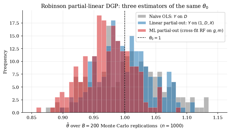
What’s the catch? Two things, both developed in detail downstream. First, the ML estimator’s good behavior depends on cross-fitting — fitting the random forest on the same data we use to compute the partial-out residuals introduces an own-fold bias that, without splitting, slowly dominates the variance reduction (§7–§8). Second, the rate at which the nuisance estimator converges has to satisfy a specific condition: $\|\hat g - g\|_{L^2(P)} \cdot \|\hat m - m\|_{L^2(P)} = o_P(n^{-1/2})$, which is satisfied if each individual nuisance converges faster than $n^{-1/4}$. Random forests on five-dimensional smooth problems clear this bar; high-dimensional sparse problems clear it only with the help of the debiased lasso (high-dimensional-regression §12.1).

The path from here: §2 sets up the geometry that lets us describe the space of all estimators (parametric submodels, tangent spaces, the $L^2(P)$ ambient), §3 picks out the efficient one inside that space (the efficient influence function), §4 quantifies the efficiency bound it achieves, and §5–§7 give us three constructive routes — one-step, TMLE, DML — to estimators that hit it.

§2. Tangent spaces

Section 2 establishes the geometric framework that organizes everything to follow. The point is to recast the “estimate a parameter while tolerating an infinite-dim nuisance” problem as a question about directions in a Hilbert space: which directions describe pure nuisance variation, which describe variation in the parameter of interest, and how do they relate. The answer is a clean orthogonal decomposition in $L^2(P)$, and the efficient influence function (§3) will turn out to be the special element of the orthogonal complement that licenses $\sqrt n$-asymptotic normality.

2.1 Parametric submodels and their score functions

A parametric submodel through $P \in \mathcal{M}$ is a one-parameter family $\{P_\epsilon : \epsilon \in (-\delta, \delta)\} \subset \mathcal{M}$ with $P_0 = P$. The submodel is regular if it’s Hellinger-differentiable: there exists $s \in L^2(P)$ — the score function — with

$$\int \left[\sqrt{dP_\epsilon} - \sqrt{dP} - \tfrac{1}{2}\epsilon\, s\, \sqrt{dP}\right]^2 \longrightarrow 0 \qquad \text{as } \epsilon \to 0.$$

For models dominated by a fixed measure $\mu$, this is equivalent to pointwise log-likelihood differentiability: $s(o) = \partial \log p_\epsilon(o)/\partial \epsilon |_{\epsilon = 0}$.

Scores have two universal properties: they’re centered ($\mathbb{E}_P[s] = 0$, from interchanging derivative and integral in $\int p_\epsilon\, d\mu \equiv 1$) and square-integrable ($\|s\|^2 < \infty$). The set of all submodel scores at $P$ is the tangent set $\mathcal{T}^*_P\mathcal{M}$. Its closed linear span (in $L^2(P)$) is the tangent space $\mathcal{T}_P\mathcal{M}$.

Robinson scores. For the partial-linear DGP, three families of submodels matter. A $\theta$-perturbation $\theta_\epsilon = \theta_0 + \epsilon$ has score $s_\theta(O) = D\varepsilon/\sigma_\varepsilon^2$. A $g$-perturbation $g_\epsilon(x) = g(x) + \epsilon h(x)$, for any $h \in L^2(P_X)$, gives $s_g[h](O) = h(X)\varepsilon/\sigma_\varepsilon^2$. An $m$-perturbation $m_\epsilon(x) = m(x) + \epsilon k(x)$, for any $k \in L^2(P_X)$, gives $s_m[k](O) = k(X)\nu/\sigma_\nu^2$.

2.2 The nuisance tangent space

For a semiparametric model $\mathcal{M} = \{P_{\theta, \eta}\}$, write $P_0 = P_{\theta_0, \eta_0}$ for the true distribution. The objects we need are two closed subspaces of $L^2_0(P_0) = \{f \in L^2(P_0) : \mathbb{E}_{P_0}[f] = 0\}$.

Robinson nuisance tangent space. Combining the three score families above (excluding for now the marginal-distribution perturbations),

$$\Lambda_\eta = \big\{h(X)\varepsilon/\sigma_\varepsilon^2 : h \in L^2(P_X)\big\} \oplus \big\{k(X)\nu/\sigma_\nu^2 : k \in L^2(P_X)\big\}.$$

The two summands are orthogonal in $L^2(P)$ because $\varepsilon$ and $\nu$ are independent and mean-zero. Each summand is itself infinite-dimensional.

2.3 The orthogonal complement and the efficient score

Robinson orthogonal complement: the efficient score. The $\theta$-score decomposes as

$$s_\theta = D\varepsilon/\sigma_\varepsilon^2 = (m(X) + \nu)\varepsilon/\sigma_\varepsilon^2 = \underbrace{m(X)\varepsilon/\sigma_\varepsilon^2}_{\in \Lambda_\eta} + \underbrace{\nu\varepsilon/\sigma_\varepsilon^2}_{\text{residual}}.$$

The first term has the form $h(X)\varepsilon/\sigma_\varepsilon^2$ with $h = m$ — a $g$-direction nuisance score, so it lives in $\Lambda_\eta$. The residual $\nu\varepsilon/\sigma_\varepsilon^2$ is uncorrelated with every nuisance score (because $\mathbb{E}[\nu] = \mathbb{E}[\varepsilon] = 0$), and so lives in $\Lambda_\eta^\perp$.

The squared $L^2$-norm of the efficient score is the efficient information: $I^*(\theta_0) = \|\ell^*_\theta\|^2 = \sigma_\nu^2/\sigma_\varepsilon^2$. The semiparametric efficiency bound for $\theta_0$ is $1/I^*(\theta_0) = \sigma_\varepsilon^2/\sigma_\nu^2$, formalized in §4. With $\sigma_\varepsilon = \sigma_\nu = 0.5$ this equals 1, so the asymptotic variance of any regular estimator of $\theta_0$ is at least $1/n = 10^{-3}$ — and the matching SD floor of $0.0316$ is exactly what §1.4 identified as the oracle target.

2.4 A finite-dimensional visual anchor

The Hilbert-space picture above is a faithful generalization of a finite-dimensional construction. Replace $L^2_0(P)$ with $\mathbb{R}^3$, the model tangent space $\mathcal{T}_{P_0}\mathcal{M}$ with a 2D plane through the origin (the tangent plane to a 2D submodel surface, in the model-as-manifold reading), and the nuisance tangent space $\Lambda_\eta$ with a 1D line within that plane. Then $\Lambda_\eta^\perp$ — taken within the tangent plane for visualization — is the perpendicular line.

Nuisance angle Λη (within tangent plane): 30°Ambient vector direction (within tangent plane): 60°

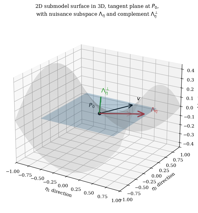
The infinite-dimensional generalization to $L^2(P)$ requires two upgrades. First, the “tangent plane” $\mathcal{T}_{P_0}\mathcal{M}$ is no longer 2D — it can be infinite-dimensional, since perturbing $g$ over $L^2(P_X)$ alone gives infinitely many independent directions. Second, “orthogonal” is now the $L^2(P)$ inner product $\langle u, v\rangle = \mathbb{E}_P[u(O)v(O)]$, computed by integrating against the true distribution. Everything else — the closed-subspace structure, the projection theorem, the uniqueness of the orthogonal decomposition — comes directly from formalCalculus: hilbert-spaces .

§3. Efficient influence functions

Section 2 gave us the geometry: $L^2_0(P)$ as the ambient, $\Lambda_\eta$ as the nuisance tangent subspace, $\Lambda_\eta^\perp$ as its orthogonal complement, and — for the Robinson partial-linear model — the efficient score $\ell^*_\theta$ as the orthogonal-to-nuisance residual of the $\theta$-score. Section 3 turns that residual into an estimator-ready object: the efficient influence function $\phi^*$. The motto: every $\sqrt n$-consistent regular estimator of $\psi(P)$ — plug-in, one-step, TMLE, DML — is asymptotically a sample average of its influence function plus an $o_P(n^{-1/2})$ remainder, and the EIF is the unique choice of influence function that minimizes the asymptotic variance. Whoever owns the EIF owns the bound.

3.1 Functionals and pathwise differentiability

A statistical functional is a map $\psi : \mathcal{M} \to \mathbb{R}^k$. For us: $\psi(P) = \theta_0$ (Robinson slope), $\psi(P) = \mathbb{E}_P[Y]$ (MAR mean), $\psi(P) = \mathbb{E}_P[Y(1) - Y(0)]$ (ATE).

Von Mises expansion. Pathwise differentiability gives a first-order Taylor expansion of $\psi$ around $P$:

$$\psi(Q) - \psi(P) = \int \phi(o; P)\, d(Q - P)(o) + R_2(Q, P),$$

where $\phi(o; P)$ is the influence function of $\psi$ at $P$ (defined precisely below) and $R_2(Q, P)$ is a second-order remainder that vanishes faster than $\|Q - P\|$ in an appropriate norm.

3.2 Influence functions

By the Riesz representation theorem on the Hilbert space $\overline{\mathcal{T}_P\mathcal{M}}^{L^2(P)}$, the continuous linear functional $\dot\psi_P$ has a unique representer — a function $\phi \in \overline{\mathcal{T}_P\mathcal{M}}^{L^2(P)}$ with

$$\dot\psi_P(s) = \langle \phi, s\rangle_{L^2(P)} = \mathbb{E}_P[\phi(O)\, s(O)] \qquad \text{for every } s \in \mathcal{T}_P\mathcal{M}.$$

This $\phi$ is the efficient influence function (EIF) of $\psi$ at $P$, written $\phi^*(\cdot; P)$.

Estimator-side definition. An estimator $\hat\theta_n$ is asymptotically linear at $P$ with influence function $\phi$ if

$$\hat\theta_n - \psi(P) = \frac{1}{n}\sum_{i=1}^n \phi(O_i) + o_P(n^{-1/2}).$$

By the CLT, $\sqrt n(\hat\theta_n - \psi(P)) \Rightarrow \mathcal{N}(0,\ \mathbb{E}_P[\phi^2])$. Regularity in the technical sense constrains an estimator’s IF to satisfy the gradient equation for $\dot\psi_P$.

3.3 The EIF as orthogonal projection

For any IF $\phi$, the projection $\phi^* = \mathrm{proj}_{\mathcal{T}_P\mathcal{M}}\phi$ is the EIF. It satisfies the gradient equation and minimizes $L^2(P)$-norm.

For a parametric target $\theta$ in a semiparametric model, with efficient score $\ell^*_\theta$ from §2:

$$\phi^*_\theta = (I^*(\theta))^{-1}\ell^*_\theta = (\|\ell^*_\theta\|^2)^{-1}\ell^*_\theta,$$

and the semiparametric efficiency bound is $1/I^*(\theta) = \|\phi^*_\theta\|^2$.

Robinson EIF. Rescale §2’s $\ell^*_\theta = \nu\varepsilon/\sigma_\varepsilon^2$ by $I^* = \sigma_\nu^2/\sigma_\varepsilon^2$:

$$\phi^*_\theta(O; P) = \frac{\nu\,\varepsilon}{\sigma_\nu^2} = \frac{(D - m(X))(Y - D\theta_0 - g(X))}{\sigma_\nu^2}.$$

The product-of-two-residuals structure (treatment residual × outcome residual) is what makes Neyman orthogonality possible in §7 — the EIF is first-order insensitive to either nuisance separately.

3.4 Worked example: EIF of the functional mean under MAR

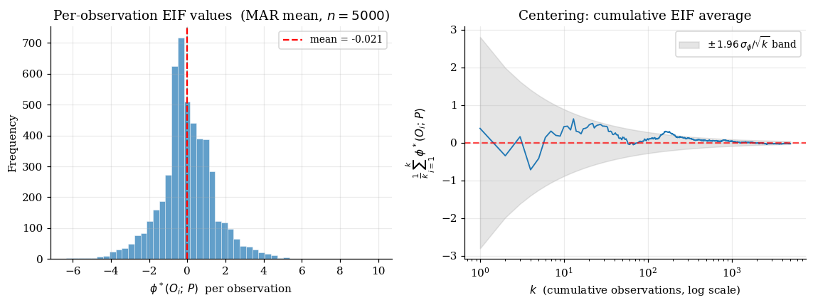
The MAR setting. Observe $O = (Y \cdot R, R, X)$ where $Y \in \mathbb{R}$, $R \in \{0, 1\}$ is the response indicator ($Y$ is recorded iff $R = 1$), and $X$ is always observed. Assume missingness at random (MAR): $Y \perp R \mid X$. Let $\pi(x) = \Pr(R = 1 \mid X = x) > 0$ (positivity), $m(x) = \mathbb{E}[Y \mid X = x, R = 1] = \mathbb{E}[Y \mid X = x]$ (the second equality from MAR). The functional of interest:

$$\psi(P) = \mathbb{E}_P[Y] = \int m(x)\, dP_X(x).$$

The fully-nonparametric model places no restrictions on $p_X$, $p_{Y \mid X}$, $p_{R \mid X}$ beyond MAR and positivity, so $\mathcal{T}_P\mathcal{M} = L^2_0(P)$.

Sample size n: 1000Compare against non-efficient IPW influence function (RY/π − ψ_IPW)

Doubly robust structure (preview for §9). Notice that $\phi^*$ has the form (outcome regression) + (IPW residual). Replace $m$, $\pi$ with arbitrary estimators $\hat m$, $\hat\pi$: as long as one is correct, the resulting one-step estimator is consistent.

3.5 The functional-delta-method perspective

A second framing — useful for connecting back to formalStatistics: empirical-processes — recasts the EIF as a Hadamard derivative of the functional $\psi$ at $P$. If $\psi$ is Hadamard-differentiable and the empirical distribution $\mathbb{P}_n$ satisfies a Donsker condition, then the functional delta method gives

$$\sqrt n\bigl(\psi(\mathbb{P}_n) - \psi(P)\bigr) = \sqrt n \int \phi^*(o; P)\, d(\mathbb{P}_n - P)(o) + o_P(1) \Rightarrow \mathcal{N}(0,\ \|\phi^*\|^2_{L^2(P)}).$$

The EIF is the Hadamard derivative of $\psi$, and it is the Riesz representer of $\dot\psi_P$, and it is the orthogonal-to-nuisance score residual. Three viewpoints, one $\phi^*$.

§4. Semiparametric efficiency bound

Section 3 constructed $\phi^*$. Section 4 turns the construction into a theorem: $\|\phi^*\|^2_{L^2(P)}$ is a lower bound on the asymptotic variance of any regular asymptotically linear (RAL) estimator of $\psi(P)$, and it’s a tight lower bound — there exist RAL estimators achieving it. This is the Bickel–Klaassen–Ritov–Wellner (1993) bound.

4.1 The Bickel–Klaassen–Ritov–Wellner lower bound

The geometric content: among all gradients (representers of the same continuous linear functional $\dot\psi_P$), the EIF is the shortest.

4.2 Information-theoretic interpretation

A complementary viewpoint frames $V_{\rm eff}$ as the inverse of the worst-case Fisher information. For any regular parametric submodel through $P$ varying $\theta$ at $\epsilon = 0$, there’s a Fisher information $I_{\rm sub}(\theta)$ for $\theta$, and the Cramér–Rao bound gives $V_\infty(\hat\theta) \geq 1/I_{\rm sub}(\theta)$. Any consistent estimator in the full model is also consistent in every submodel, so:

$$V_\infty(\hat\theta_n) \geq \sup_{\text{submodels}} \frac{1}{I_{\rm sub}(\theta)} = \frac{1}{\inf_{\text{submodels}} I_{\rm sub}(\theta)} = \frac{1}{I^*(\theta)}.$$

The hardest submodel to estimate $\theta$ in is the one orthogonal to the nuisance — that’s where the score for $\theta$ has the least “room” left after the nuisance soaks up its share.

For Robinson partial-linear with Gaussian noise: $I^*(\theta_0) = \sigma_\nu^2/\sigma_\varepsilon^2$, so $V_{\rm eff} = \sigma_\varepsilon^2/\sigma_\nu^2$. For the MAR mean (§3.4): $V_{\rm eff} = \mathrm{Var}(m(X)) + \mathbb{E}[\sigma^2(X)/\pi(X)]$, where $\sigma^2(x) = \mathrm{Var}(Y \mid X = x)$.

4.3 Recovery of Cramér–Rao when $\Lambda_\eta = \{0\}$

When the model is fully parametric — $\theta$ the only unknown — the nuisance tangent space collapses: $\Lambda_\eta = \{0\}$. Projection onto $\Lambda_\eta$ is the zero map, so $\ell^*_\theta = s_\theta$, $I^*(\theta) = I(\theta)$, and $V_{\rm eff} = 1/I(\theta)$ — the Cramér–Rao bound. The simplest example: $Y_i \sim \mathcal{N}(\theta, \sigma^2)$ with known $\sigma^2$. Score $s_\theta(y) = (y - \theta)/\sigma^2$, Fisher info $I = 1/\sigma^2$, CR bound $\sigma^2$. The semiparametric bound matches.

In general, adding nuisance directions can only enlarge $\Lambda_\eta$, which can only decrease $I^*(\theta) = I(\theta) - \|\mathrm{proj}_{\Lambda_\eta} s_\theta\|^2$, which can only increase the bound. The price you pay for not knowing the nuisance is the squared length of the projection of $s_\theta$ onto $\Lambda_\eta$.

4.4 Numerical demonstration

Monte-Carlo replications B: 100

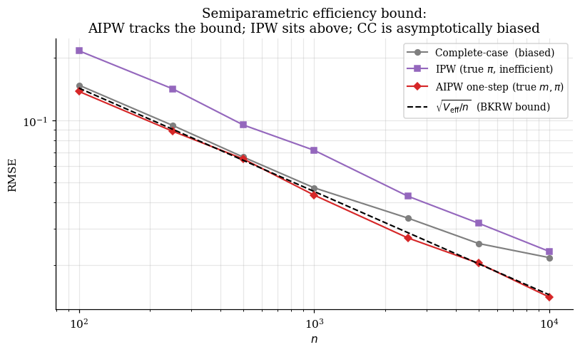
The bound is tight: there exist RAL estimators with $V_\infty = V_{\rm eff}$. The next three sections give three constructions — one-step (§5), TMLE (§6), and DML (§7) — all asymptotically equivalent under standard regularity but with different finite-sample profiles.

Failure modes. The bound is not achieved when the model is irregular, when the nuisance estimator’s rate is too slow ($\|\hat\eta - \eta\|_{L^2(P)} = \omega_P(n^{-1/4})$ — the rate condition §7 makes rigorous and §8 demonstrates empirically), or when the plug-in $\psi(\hat P)$ is not pathwise-differentiable in a regime where the alternative constructions also struggle.

§5. One-step estimators

The von Mises expansion (§3.1) makes the plug-in’s first-order bias precise:

$$\psi(P) - \psi(\hat P) = \mathbb{E}_P[\phi^*(O; \hat P)] + R_2(P, \hat P).$$

The plug-in error is, up to second order, the EIF’s expectation under the true distribution evaluated at the fitted nuisance. We can’t compute this expectation directly, but we can estimate it from data.

5.1 The EIF correction recipe

Estimate $\mathbb{E}_P[\phi^*(O; \hat P)]$ by $\mathbb{P}_n[\phi^*(\cdot; \hat P)] = n^{-1}\sum_i \phi^*(O_i; \hat P)$. Then the one-step estimator is the plug-in plus this empirical correction:

$$\hat\psi_{1\text{-}{\rm step}} = \psi(\hat P) + \mathbb{P}_n[\phi^*(\cdot; \hat P)] = \psi(\hat P) + \frac{1}{n}\sum_{i=1}^n \phi^*(O_i; \hat P).$$

For the MAR mean this unrolls to the familiar AIPW form:

$$\hat\psi^{\rm MAR}_{1\text{-}{\rm step}} = \underbrace{\frac{1}{n}\sum_i \hat m(X_i)}_{\text{outcome-regression plug-in}} + \underbrace{\frac{1}{n}\sum_i \frac{R_i(Y_i - \hat m(X_i))}{\hat\pi(X_i)}}_{\text{IPW-residual correction}}.$$

Three readings of the same construction. Bias correction: the EIF correction estimates and subtracts the plug-in’s first-order bias. Estimating equation: $\hat\psi_{1\text{-}{\rm step}}$ solves the empirical version of the EIF moment condition. Score adjustment: in the parametric MLE special case ($\Lambda_\eta = \{0\}$), the one-step is the classical Newton–Raphson step from a $\sqrt n$-consistent starting estimate toward the MLE.

5.2 Asymptotic normality under the rate condition

The rate condition unpacked. For AIPW-style functionals the von Mises remainder has a product-of-errors form:

$$R_2(\hat P, P) = \int (\hat m(x) - m(x))\bigl(\hat\pi(x) - \pi(x)\bigr) \cdot \omega(x)\, dP_X(x) + o_P(\cdots),$$

where $\omega(x) > 0$ is a known weight. By Cauchy–Schwarz, $|R_2| \leq C \cdot \|\hat m - m\|_{L^2} \cdot \|\hat\pi - \pi\|_{L^2}$. So the rate condition reduces to

$$\|\hat m - m\|_{L^2} \cdot \|\hat\pi - \pi\|_{L^2} = o_P(n^{-1/2}).$$

A sufficient (and convenient) condition: both nuisances converge at rates faster than $n^{-1/4}$. Random forests on smooth low-to-moderate-dimensional problems clear this threshold; the debiased lasso clears it in sparse high-dimensional regimes.

5.3 Numerical verification on the MAR mean

We run the one-step estimator on the §3.4 MAR DGP with $n = 1000$ and $B = 200$ MC replications, using well-specified parametric nuisance fits.

MC replications B: 200

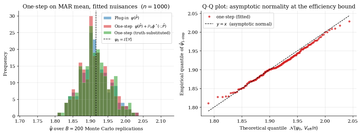
The one-step with fitted nuisances has empirical standard deviation close to $\sqrt{V_{\rm eff}/n}$ — the BKRW bound — and the rate-condition gap (between fitted and truth-substituted one-step) is at the Monte Carlo noise floor, confirming that well-specified parametric nuisances pay no asymptotic price.

§6. Targeted maximum likelihood (TMLE)

The one-step recipe (§5) adds an external EIF correction to the plug-in: $\hat\psi_{1\text{-}{\rm step}} = \psi(\hat P) + \mathbb{P}_n[\phi^*(\cdot; \hat P)]$. The output is a number, not a plug-in of any probability distribution. TMLE (van der Laan & Rubin 2006; van der Laan & Rose 2011) takes a different mechanical route to the same asymptotic destination: it updates the distribution $\hat P$ to $\hat P^*$ along a carefully chosen parametric submodel until the empirical EIF correction vanishes — $\mathbb{P}_n[\phi^*(\cdot; \hat P^*)] = 0$ — so the plug-in $\psi(\hat P^*)$ is already efficient.

6.1 Iterative fluctuation

A fluctuation of $\hat P$ in direction $\phi^*$ is a one-parameter family $\{\hat P_\epsilon\}$ with $\hat P_0 = \hat P$ and score parallel to $\phi^*(\cdot; \hat P)$ at $\epsilon = 0$. The targeting step picks $\hat\epsilon$ by maximum likelihood over the fluctuation, producing $\hat P^* = \hat P_{\hat\epsilon}$. By construction, the MLE first-order condition for $\hat\epsilon$ is exactly $\mathbb{P}_n[\phi^*(\cdot; \hat P^*)] = 0$.

6.2 The targeting step: closed-form fluctuation for AIPW

For functionals whose EIF has the AIPW structure $\phi^*(O; P) = m(X) - \psi + H(X) R (Y - m(X))$ with $H$ a clever covariate, the fluctuation acts on the outcome regression $\hat m$ by adding a multiple of $H$:

$$\hat m_\epsilon(x) = \hat m_0(x) + \epsilon \cdot H(x) \qquad \text{(linear fluctuation, continuous Y).}$$

For the MAR mean (§3.4), the clever covariate is $H(x) = 1/\pi(x)$. For the ATE under unconfoundedness, the clever covariate for the treated branch is $H_1(x) = D/\pi(x)$ and for the control branch $H_0(x) = -(1-D)/(1-\pi(x))$.

Continuous Y (linear fluctuation, closed form). The MLE of $\epsilon$ under Gaussian likelihood is OLS of the residual $Y - \hat m_0(X)$ on $H(X)$, restricted to observed cases:

$$\hat\epsilon = \frac{\sum_{i:\, R_i = 1} H(X_i)(Y_i - \hat m_0(X_i))}{\sum_{i:\, R_i = 1} H(X_i)^2}.$$

The updated regression is $\hat m^*(x) = \hat m_0(x) + \hat\epsilon \cdot H(x)$, and the TMLE estimator is $\hat\psi_{\rm TMLE} = n^{-1} \sum_i \hat m^*(X_i)$.

Why this works. The fluctuation’s score at $\epsilon = 0$ is proportional to $H(X) R (Y - \hat m_0(X))$ — the AIPW residual term of $\phi^*$. The score equation for $\hat\epsilon$ therefore reads $\mathbb{P}_n[H(X) R (Y - \hat m^*(X))] = 0$, which is the empirical version of the EIF correction being zero. Targeting in the AIPW direction forces the AIPW residual to vanish empirically, and the plug-in $\psi(\hat P^*)$ inherits the EIF correction via the distribution update.

6.3 The substitution-estimator property

TMLE’s defining structural feature: $\hat\psi_{\rm TMLE} = \psi(\hat P^*)$ is a plug-in of an actual probability distribution. Whatever range or constraints $\psi$ inherits from probability distributions in $\mathcal{M}$, $\hat\psi_{\rm TMLE}$ inherits them automatically.

The contrast with one-step is sharpest for bounded parameters. Take a binary-outcome ATE: $\psi(P) \in [-1, 1]$. The one-step estimator — a number, not a distribution plug-in — has no boundedness guarantee. TMLE doesn’t: the logistic fluctuation keeps $\hat m^*(x) \in (0, 1)$ at every point, so the plug-in stays in $[-1, 1]$ by construction.

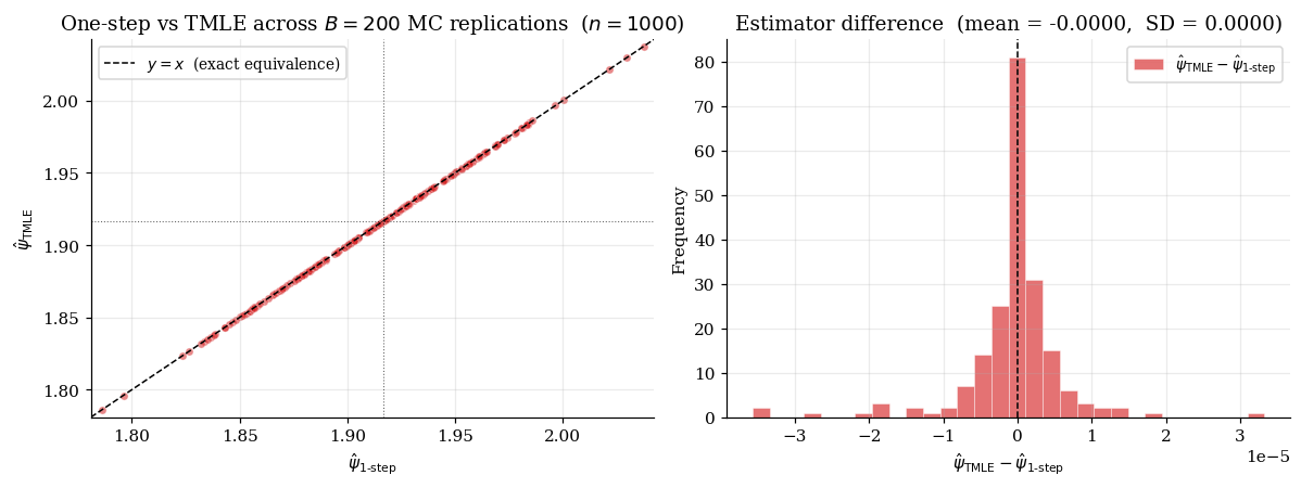
6.4 Asymptotic equivalence to the one-step estimator

MC replications B: 100

6.5 Where TMLE beats one-step in finite samples

Three regimes where TMLE empirically outperforms one-step:

Extreme propensities. When $\hat\pi(x)$ approaches 0 or 1 for some $x$, the clever covariate $H(x) = 1/\hat\pi(x)$ explodes. TMLE’s targeting step regularizes this via the $H^2$ denominator in $\hat\epsilon$.

Bounded parameters. Binary-outcome ATEs, success rates, win probabilities — anything in a bounded interval. TMLE’s substitution form respects the bounds; one-step doesn’t.

Heavy-tailed residuals. TMLE’s update is OLS- or logistic-MLE-derived, weighting residuals less heavily in the tails than the one-step sample-mean correction.

The cost: TMLE is one extra fitting step per estimate, and the implementation is functional-specific. For straightforward AIPW functionals — MAR mean, ATE, partial-linear slope — the cost is negligible.

§7. Double / debiased machine learning (DML)

The §5.3 theorem as stated doesn’t apply directly to random forests, gradient-boosted trees, deep networks, or lasso in high dimensions — none of these sit inside a Donsker class with probability 1. Double / debiased machine learning (DML; Chernozhukov et al. 2018) is the modern repair: replace the Donsker condition with a cross-fitting protocol, and use the Neyman orthogonality of the EIF-based moment to keep the rate condition lenient enough that $n^{-1/4}$-rate ML nuisance is sufficient.

7.1 Neyman orthogonality

Let $\psi(O; \theta, \eta)$ be a moment function satisfying $\mathbb{E}_{P_0}[\psi(O; \theta_0, \eta_0)] = 0$.

The connection to the EIF. The efficient score $\ell^*_\theta$ is, by §2’s construction, orthogonal to every nuisance score $s \in \Lambda_\eta$ in the $L^2(P)$ inner product. The directional derivative of $\mathbb{E}_{P_0}[\ell^*_\theta(O)]$ along a submodel with nuisance score $s$ is exactly $\langle \ell^*_\theta, s\rangle_{L^2(P)} = 0$. So $\ell^*_\theta$ — and any score-based moment derived from it, including the EIF-based DML moment — is Neyman-orthogonal.

Verifying for the AIPW moment $\psi^{\rm AIPW}(O; \theta, \eta) = m(X) - \theta + H(X) R (Y - m(X))$:

Perturbing $m$ in direction $h$: $\partial_m \mathbb{E}_{P_0}[\psi^{\rm AIPW}][h] = \mathbb{E}[h(X) - H(X) R h(X)] = \mathbb{E}[h(X)(1 - \pi_0(X) H(X))]$. For the MAR mean $H = 1/\pi_0$, so $\pi_0 H = 1$ and the bracket is zero.

Perturbing $\pi$ in direction $k$: $\partial_\pi \mathbb{E}_{P_0}[\psi^{\rm AIPW}][k] = \mathbb{E}[\partial_\pi H[k] \cdot R(Y - m_0(X))]$. By MAR, $\mathbb{E}[R(Y - m_0) \mid X] = 0$, so this vanishes.

Both directional derivatives vanish at $\eta_0$. AIPW is Neyman-orthogonal at the truth.

7.2 The product-of-errors second-order remainder

For the AIPW moment with $\eta = (m, \pi)$, the expansion at $\hat\eta$ near $\eta_0$ gives

$$\mathbb{E}_{P_0}[\psi^{\rm AIPW}(O; \theta_0, \hat\eta)] = R_2(\hat\eta, \eta_0).$$

For the MAR mean, a direct calculation gives

$$R_2(\hat\eta, \eta_0) = \mathbb{E}_{P_0}\!\left[(\hat m(X) - m_0(X))\cdot \frac{\hat\pi(X) - \pi_0(X)}{\hat\pi(X)}\right].$$

By Cauchy–Schwarz, assuming $\hat\pi \geq c > 0$ (positivity),

$$|R_2(\hat\eta, \eta_0)| \leq \frac{1}{c}\cdot \|\hat m - m_0\|_{L^2(P_X)}\cdot \|\hat\pi - \pi_0\|_{L^2(P_X)}.$$

Product of $L^2$-errors. The remainder is bounded by the product of the nuisance errors, not by either alone. This is what makes ML-rate nuisance survive: each individual error can be $O_P(n^{-1/4})$ and the product still satisfies $\|\hat m - m\| \cdot \|\hat\pi - \pi\| = O_P(n^{-1/2})$, exactly what §5.3’s CLT needs.

7.3 The $o_P(n^{-1/4})$ rate condition

Combining Neyman orthogonality with the product-of-errors $R_2$ gives the DML rate condition:

$$\|\hat m - m_0\|_{L^2(P)}\cdot \|\hat\pi - \pi_0\|_{L^2(P)} = o_P(n^{-1/2}).$$

When the two errors are at comparable rates $\alpha_m = \alpha_\pi = \alpha$, this reduces to $\alpha > 1/4$. Each nuisance separately needs $o_P(n^{-1/4})$. This is dramatically more lenient than parametric MLE’s $n^{-1/2}$.

Where the $n^{-1/4}$ comes from. Without Neyman orthogonality, the first-order term in the von Mises expansion of $\mathbb{E}[\psi(\theta_0, \hat\eta)]$ is $O(\|\hat\eta - \eta_0\|)$, requiring $o(n^{-1/2})$ rates. Neyman orthogonality kills that first-order term, leaving only the second-order remainder $O(\|\hat\eta - \eta_0\|^2)$, requiring only $o(n^{-1/4})$.

ML rates clear the threshold. Random forests on $s$-smooth $d$-dimensional regression functions achieve roughly $n^{-1/(2 + d/s)}$ — at $d = 5$, $s = 4$, this is $n^{-1/3}$, beating $n^{-1/4}$. The debiased lasso (high-dimensional-regression §12.1) achieves $\sqrt{s \log p / n}$ in sparse $p$-dimensional regimes — at $s = O(\sqrt n)$, this is $n^{-1/4}\sqrt{\log p}$, marginal but sufficient.

7.4 Two canonical DML examples

Average treatment effect under unconfoundedness. Observe $(Y, D, X)$ with binary $D$ and unconfoundedness $(Y(1), Y(0)) \perp D \mid X$ (with positivity). The AIPW moment:

$$\psi^{\rm ATE}(O; \theta, \mu_1, \mu_0, \pi) = \mu_1(X) - \mu_0(X) + \frac{D(Y - \mu_1(X))}{\pi(X)} - \frac{(1 - D)(Y - \mu_0(X))}{1 - \pi(X)} - \theta.$$

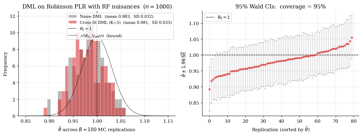
Partial-linear regression (Robinson 1988).

$$\psi^{\rm PLR}(O; \theta, g, m) = (D - m(X))(Y - D\theta - g(X)),$$

solved for $\hat\theta = \mathbb{P}_n[(D - \hat m)\, Y]/\mathbb{P}_n[(D - \hat m)(D - \hat m)]$ after substituting $g \to \hat g$.

Folds K: 2 5 10

MC replications B: 100

§8. Sample-splitting and cross-fitting

§7 stated that DML with ML nuisance sidesteps the §5.3 Donsker condition via cross-fitting. §8 develops the protocol.

8.1 Why naive plug-in with ML nuisance over-fits

Fit $\hat g$, $\hat m$ on the full sample, then compute the partial-linear OLS slope from the residuals. ML estimators are designed to minimize training error on the full sample. Training-error minimization for $\hat g$ reduces $\{Y_i - \hat g(X_i)\}$ on training points — including structure that belongs to $\theta_0 D$ rather than the nuisance $g(X)$. The result: residuals on the training data are systematically smaller than residuals would be on fresh data, and the partial-linear OLS slope inherits the bias.

The §5.3 equicontinuity condition fails for ML nuisance because $\hat\eta$ depends on the same data $\mathcal{D}$ that the empirical process is averaging over.

8.2 The K-fold cross-fitting protocol

Chernozhukov et al. (2018) Algorithm DML2:

1. Partition. Randomly partition $\{1, \ldots, n\}$ into $K$ disjoint folds $I_1, \ldots, I_K$.
2. Cross-fit. For each fold $k$, fit $\hat\eta^{(-k)}$ on $\mathcal{D}_{-k}$, then compute cross-fit residuals $\tilde Y_i = Y_i - \hat g^{(-k)}(X_i)$ and $\tilde D_i = D_i - \hat m^{(-k)}(X_i)$ for $i \in I_k$.
3. Stack and solve. Combine the cross-fit residuals across all folds and solve the DML moment equation:

$$\hat\theta_{\rm DML} = \frac{\sum_i \tilde D_i \tilde Y_i}{\sum_i \tilde D_i^2} \qquad \text{(partial-linear case).}$$

4. Standard error. The sandwich SE uses the EIF at the stacked residuals.

8.3 The bias-variance trade-off in K

K = 2. Half the data trains the nuisance; the other half computes the moment. Maximally simple, but each fold’s nuisance is fit on only $n/2$ observations.

K = 5. Each fold’s nuisance is fit on $4n/5$ observations — close to full-sample efficiency for the nuisance, while still keeping the cross-fit residuals independent of the nuisance fit. The default in econml, doubleml.

K = 10 or larger. Marginal additional accuracy, at higher computational cost.

The asymptotics don’t depend on $K$ — every fixed $K$ gives the same $V_{\rm eff}$ limit — but finite-sample behavior does. The notebook uses $K = 5$ throughout.

8.4 The empirical stress test of the rate condition

Take the partial-linear DGP and replace the nuisance estimators with the truth plus controlled-rate noise: $\hat g(x) = g_0(x) + \varepsilon_g$, $\hat m(x) = m_0(x) + \varepsilon_m$, where $\varepsilon_g$, $\varepsilon_m \sim \mathcal{N}(0, n^{-2\alpha})$ i.i.d. The $L^2$ error of each nuisance is exactly $n^{-\alpha}$, by construction. We sweep $\alpha \in \{0.10, 0.15, 0.20, 0.25, 0.30, 0.40, 0.50\}$ across the rate threshold.

For $\alpha > 1/4$: product of errors $n^{-2\alpha} = o(n^{-1/2})$, rate condition holds, coverage $\approx 0.95$. For $\alpha < 1/4$: product $\succ n^{-1/2}$, rate condition violated, asymptotic CLT breaks. Coverage drops sharply.

MC replications B per α: 100

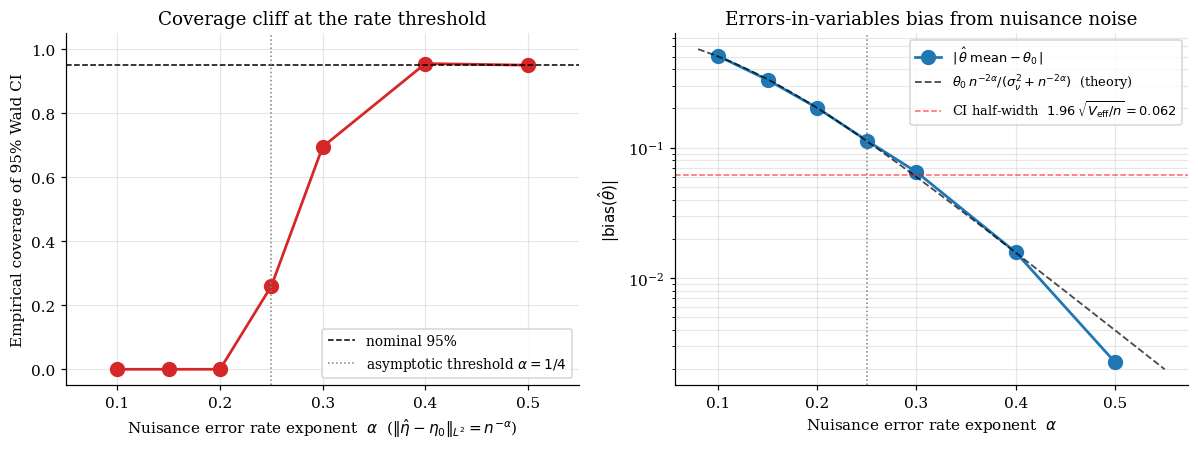
The rate condition is binding, not aspirational. Slow nuisance rates produce undercoverage that cross-fitting cannot rescue — only a faster nuisance estimator can.

§9. Worked examples

Sections 5 through 8 built the full machinery. Section 9 takes the toolkit and runs it through three substantive examples and one forward-pointer stub.

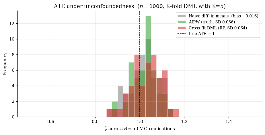
9.1 ATE under unconfoundedness

The setup. Observe $O = (Y, D, X)$ with $D \in \{0, 1\}$ a binary treatment and $X$ pre-treatment covariates, unconfoundedness $(Y(1), Y(0)) \perp D \mid X$, and positivity $\pi(X) \in (\delta, 1 - \delta)$.

The EIF (AIPW form):

$$\phi^*(O; P) = \mu_1(X) - \mu_0(X) + \frac{D(Y - \mu_1(X))}{\pi(X)} - \frac{(1 - D)(Y - \mu_0(X))}{1 - \pi(X)} - \psi(P).$$

This is the causal-inference-methods §6 estimator viewed as a specific instance of the §3 construction.

Three estimators on a simulated DGP. Take $X \sim U([0, 1]^5)$, $\pi(x) = \sigma(0.5 - x_1 + 0.5 x_2)$, $\mu_0(x) = 1 + 0.5 x_1 + x_2^2$, $\mu_1(x) = \mu_0(x) + 1$ (constant treatment effect, so the true ATE is 1.0). The notebook produces a three-histogram comparison.

MC replications B: 100

What to look forThe naive estimator (grey) is biased — the histogram center sits off the true ATE=1 because D and X are confounded. AIPW with truth-substituted nuisances (red) is unbiased and asymptotically efficient. Cross-fit DML with polynomial nuisance (purple) approaches the same efficient distribution as B grows, demonstrating that ML-fitted nuisance clears the rate condition on this smooth DGP.

9.2 Robinson partial-linear with local-cubic nuisance

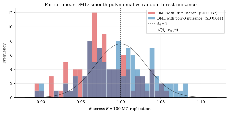
The setup is unchanged from §1.3 and §7. What changes is the nuisance estimator: §9.2 uses polynomial regression of degree 3 with full interactions — a smooth, low-bias, parametric-but-flexible estimator that approximates a “local cubic” fit. This is the strategic-doc forward-pointer from local-regression §12.1: smooth nonparametric nuisance estimators clear the DML rate threshold.

Why polynomial-of-degree-3? A polynomial of degree 3 — with all 5-dimensional interactions, 55 features at degree 3 (excluding bias) — approximates the smooth $g$ and $m$ closely. The remaining approximation error is well below $n^{-1/4}$ at $n = 1000$.

Nuisance: linear poly3 oracle

MC replications B (top panel only): 100

9.3 Functional mean under MAR (end-to-end synthesis)

The MAR-mean example has been developed across §3.4 (EIF), §5.4 (one-step), §6.4 (TMLE), and §7 (AIPW connection). §9.3 is the end-to-end synthesis with K=5 cross-fitting.

The sandwich SE for the MAR mean follows the §10 recipe. The Wald CI $\hat\psi \pm 1.96 \cdot \widehat{\rm SE}(\hat\psi)$ has empirical coverage ≈ 94% across MC replications at $n = 1000$ (slightly below nominal due to finite-sample undercoverage typical of asymptotic CIs).

9.4 Quantile treatment effects (forward-pointer stub)

For quantile treatment effects — $\tau_q = F^{-1}_{Y(1)}(q) - F^{-1}_{Y(0)}(q)$ — the semiparametric construction proceeds through the same EIF machinery but uses the quantile regression moment in place of the conditional mean. The relevant influence-function derivation lives in quantile-regression (coming soon). The DML rate condition takes the same form, and the cross-fitting protocol of §8 carries over unchanged.

§10. Inference and confidence intervals

§5–§9 built point estimators that achieve the BKRW bound. §10 turns point estimates into honest confidence statements.

10.1 Sandwich variance from the EIF

The general Z-estimator $\hat\theta$ solves $\mathbb{P}_n[\psi(O; \hat\theta, \hat\eta)] = 0$. Standard asymptotic-linearity analysis gives

$$\sqrt n(\hat\theta - \theta_0) = -A_0^{-1} \sqrt n\, \mathbb{P}_n[\psi(O; \theta_0, \eta_0)] + o_P(1),$$

where $A_0 = \mathbb{E}[\partial_\theta \psi(O; \theta_0, \eta_0)]$ is the Jacobian. By CLT, $\sqrt n \mathbb{P}_n \psi \Rightarrow \mathcal{N}(0, B_0)$ with $B_0 = \mathrm{Var}[\psi]$. Therefore

$$\sqrt n(\hat\theta - \theta_0) \Rightarrow \mathcal{N}(0, A_0^{-2} B_0).$$

The sandwich variance estimator:

$$\widehat V = \hat A_n^{-2} \hat B_n, \qquad \hat A_n = \mathbb{P}_n\, \partial_\theta \psi(\hat\theta, \hat\eta), \qquad \hat B_n = \mathbb{P}_n[\psi(\hat\theta, \hat\eta)^2].$$

For EIF-based moments specifically. When $\psi = \phi^* - (\theta - \psi(P))$ — the AIPW form — the Jacobian collapses: $A_0 = -1$, and $\widehat V_{\rm eff} = n^{-1} \sum_i (\hat\phi^*_i - \hat\theta)^2$. This is the sample variance of the cross-fit empirical EIF.

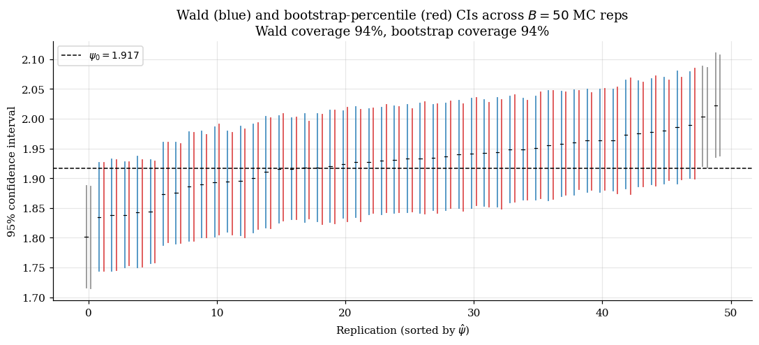
10.2 Wald intervals and their nominal coverage

The standard Wald $(1 - \alpha)$-CI: $\mathrm{CI}_{\rm Wald}(\alpha) = \hat\theta \pm z_{1 - \alpha/2} \cdot \widehat{\rm SE}(\hat\theta)$. Under asymptotic normality and consistent $\widehat V$, this has asymptotic coverage $1 - \alpha$.

At finite sample sizes, the empirical coverage is typically slightly below nominal — undercoverage of 1–2 percentage points at $n = 1000$ — for three composable reasons: skewness in the EIF distribution, $\widehat{\rm SE}$‘s own $O(n^{-1/2})$ error, and finite-sample nuisance noise.

Propensity trimming. The EIF for AIPW-style functionals can have heavy tails when the propensity approaches 0 or 1. Standard practice clips $\hat\pi$ at $[c, 1 - c]$ for small $c$ (typical: 0.05).

10.3 Multiplier bootstrap

Compute the cross-fit empirical EIF $\hat\phi^*_i$ once. Draw multiplier weights $W^b$ from a mean-zero, unit-variance distribution (typical: the two-point Mammen distribution $W_i \in \{(1 - \sqrt 5)/2,\ (1 + \sqrt 5)/2\}$ with probabilities $(5 + \sqrt 5)/10$ and $(5 - \sqrt 5)/10$) and compute the bootstrap estimate

$$\hat\theta^*_b = \hat\theta + \frac{1}{n}\sum_{i = 1}^n W_i^b\,(\hat\phi^*_i - \hat\theta).$$

Centering the influence function ($\hat\phi^*_i - \hat\theta$) is essential: with $E[W] = 0$ and $\mathrm{Var}(W) = 1$, the bootstrap variance equals the sandwich variance asymptotically. The multiplier bootstrap costs $O(n B_{\rm boot})$ — essentially free even with $B_{\rm boot} = 10000$.

Polynomial-degree-3 nuisance (uncheck for linear-control nuisance)MC replications B per n: 80

10.4 What fails when the rate condition is violated

The sandwich SE estimates variance, not bias. When the rate condition is violated, $\hat\theta$ is no longer centered at $\theta_0$, and the Wald CI $\hat\theta \pm 1.96\, \widehat{\rm SE}$ has the right width but the wrong center.

The bootstrap doesn’t fix this. Both empirical and multiplier bootstrap approximate the sampling distribution of $\hat\theta$, which already includes the rate-violation bias.

The cure is diagnostic, not inferential. When the rate condition is in doubt, check the nuisance estimator’s empirical rate via cross-validated nuisance MSE. If the empirical rate clears the threshold with comfortable margin, the Wald CI is honest. If it doesn’t, no SE construction will rescue the coverage.

§11. Connections to uncertainty quantification

§11 realizes the forward-pointer from uncertainty-quantification §14.1 — “EIF correction for asymptotically optimal estimators of variance/uncertainty parameters”. The §3 EIF construction applies to variance functionals (not just mean functionals) by the same machinery, and the resulting one-step estimator equals the cross-fit plug-in.

11.1 The EIF correction for a variance functional

Take the regression model $Y = m_P(X) + \varepsilon$ with $\mathbb{E}_P[\varepsilon \mid X] = 0$ and irreducible noise variance $\sigma^2(x) = \mathrm{Var}_P(Y \mid X = x)$. The marginal residual variance — the relevant aleatoric-uncertainty parameter — is

$$\psi(P) = \mathbb{E}_P[(Y - m_P(X))^2] = \mathbb{E}_P[\sigma^2(X)].$$

Deriving the EIF. Apply §3’s machinery in the fully nonparametric model. After grouping terms, the gradient along a $p_{Y \mid X}$-direction submodel collapses to $\mathbb{E}_P[(Y - m_P(X))^2 t(Y, X)]$, so by Riesz representation:

$$\phi^*(O; P) = (Y - m_P(X))^2 - \psi(P).$$

Centered residual-squared. Variance $\|\phi^*\|^2 = \mathrm{Var}_P[(Y - m_P(X))^2]$, the BKRW efficiency bound for estimating $\psi$.

The one-step estimator collapses to the cross-fit plug-in. Applying §5’s recipe with cross-fit nuisance $\hat m^{(-k(i))}$:

$$\hat\psi_{1\text{-}{\rm step}} = \frac{1}{n}\sum_i (Y_i - \hat m^{(-k(i))}(X_i))^2 + \frac{1}{n}\sum_i \bigl[(Y_i - \hat m^{(-k(i))}(X_i))^2 - \hat\psi\bigr].$$

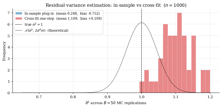
Substituting $\hat\psi = \hat\psi_{\rm cf} := n^{-1} \sum_i (Y_i - \hat m^{(-k(i))}(X_i))^2$, the second sum is identically zero. The one-step estimator equals the cross-fit plug-in. The EIF construction tells us not that we need an explicit add-on correction (as in AIPW) but that cross-fit residuals are the right ingredient.

11.2 Plug-in vs EIF-corrected variance: bias reduction

The numerical demo. Take a regression DGP $Y = f(X) + \varepsilon$ with $X \sim U([0, 1]^5)$, $f(x) = 1 + x_1 + x_2^2 + \sin(\pi x_3)$, $\varepsilon \sim \mathcal{N}(0, 1)$, so $\sigma^2 = 1$.

The in-sample plug-in fit on full data has residuals that are systematically smaller than out-of-sample residuals, so $\hat\sigma^2_{\rm in}$ is biased downward. The cross-fit one-step is unbiased and efficient.

MC replications B: 80

11.3 Semiparametric-efficient calibration

The standard frequentist recipe for calibrating prediction intervals in regression problems is to use out-of-sample residual variance — typically via cross-validation or a held-out test set. The §11 development shows this recipe is exactly the semiparametric-efficient estimator of $\sigma^2$: the cross-fit residual variance is the EIF-based one-step estimator, achieving the BKRW bound.

This is the pedagogical synthesis. Different research communities have arrived at the same recipe — cross-fit residuals for calibration — via different theoretical lenses. The semiparametric framework places the recipe in a unified construction that applies to mean, variance, quantile, and ATE-style functionals.

§12. Connections to causal inference

causal-inference-methods developed AIPW, TMLE, and DML as procedures on the ATE, LATE, front-door, and sensitivity analysis. §12 closes the loop: the procedures there are instances of the abstract framework built up across §2–§8.

12.1 The abstract framework underneath AIPW / TMLE / DML

The semiparametric framework reorganizes the procedural catalog around a single pipeline:

1. Identify the target functional $\psi : \mathcal{M} \to \mathbb{R}^k$ on the relevant model (incorporating the identifying assumptions).
2. Compute the EIF $\phi^*$ by §3’s recipe.
3. Construct the one-step / TMLE / DML estimator using $\phi^*$, with cross-fitting for ML nuisance.
4. Standard errors from the §10 sandwich; Wald CIs.

Steps 1 and 2 are estimand-specific; steps 3 and 4 are universal. The ATE-AIPW formula in causal-inference-methods §6 is what step 2 produces when $\psi(P) = \mathbb{E}_P[Y(1) - Y(0)]$ — same equation, different derivation route.

The double-robustness property — consistency under correctness of either the outcome regression or the propensity — is the structural fact that the EIF’s $R_2$ remainder has product-of-errors form (§7.2): one factor zero kills $R_2$, hence consistency.

12.2 What this layer adds

First, generality. The §3 EIF construction is functional-agnostic. The same apparatus produces AIPW for the ATE, the MAR-mean EIF (§3.4), the residual-variance EIF (§11.1), Robinson’s partial-linear EIF (§7.1), quantile-treatment-effect EIFs, and indefinitely many other targets. Semiparametric inference is not a causal-inference framework — it’s an estimation-and-inference framework that happens to subsume the relevant causal estimands as instances.

Second, the lower bound. The BKRW theorem (§4.1) supplies a concrete target: $\|\phi^*\|^2$. The §4 demonstration that the bound is achievable, plus the §7 demonstration that DML hits the bound with ML nuisance, give a clear story: the best you can do on any pathwise-differentiable estimand is to use the EIF-based one-step or its equivalents.

Third, the rate condition as a constraint, not an asymptotic afterthought. The §7.3 derivation of $\|\hat\eta_1 - \eta_1\| \cdot \|\hat\eta_2 - \eta_2\| = o_P(n^{-1/2})$ plus the §8 empirical stress test transform the rate condition from a regularity-assumption footnote into a concrete diagnostic the practitioner has to engage with.

12.3 IV / front-door / sensitivity pointer-back

Three named estimands in causal-inference-methods deserve explicit pointer-backs:

Instrumental variables (LATE). The Imbens–Angrist (1994) LATE under one-sided non-compliance has an EIF combining the instrument propensity, the compliance-class-conditional outcome regression, and the Wald-ratio structure of LATE identification. The construction follows §3’s recipe applied to the LATE-identification model.

Front-door identification. When unconfoundedness is unavailable but a mediator $M$ satisfies the front-door criterion, the ATE is identified via a mediator-distribution-plus-outcome-given-mediator formula. The EIF combines two nuisance components.

Sensitivity analysis for unobserved confounding. When unconfoundedness is suspect, sensitivity analysis bounds the parameter over admissible deviations. The §10 sandwich SE remains valid pointwise within the bound.

For each, the abstract construction is identical to the §5–§8 mechanics in this topic. Practitioners working in these regimes can apply the §5–§8 toolkit once the EIF is in hand from causal-inference-methods.

§13. Computational notes

13.1 econml and causalml as production references

For the named causal estimands in §9, two Python packages cover the production case with high quality.

econml (Microsoft Research). Implements DML for ATE under unconfoundedness, partial-linear regression, LATE under IV, and several heterogeneous-treatment-effect estimators. Native support for cross-fitting, scikit-learn-compatible nuisance learners, and sandwich SEs.

causalml (Uber). Comparable scope, with stronger emphasis on uplift modeling and conditional ATE estimation.

doubleml (Bach, Chernozhukov, Kurz, Spindler 2022). The R-and-Python implementation closest to the canonical theory. Useful for verification when an implementation choice is in doubt.

13.2 Nuisance-rate diagnostics in practice

Held-out validation MSE. Hold out a fraction $\alpha$ of the data; fit the nuisance on the remaining $1 - \alpha$; evaluate MSE on the held-out fold. If the held-out MSE decays like $n^{-\beta}$ for $\beta > 1/4$ as $n$ grows, the rate condition is plausibly satisfied.

Cross-validated MSE. When data is scarce, $K$-fold cross-validation of nuisance MSE is the practical alternative.

Diagnostic limits. Both diagnostics estimate the empirical rate, not the asymptotic rate. At moderate $n$, the diagnostic is suggestive rather than dispositive.

Practical rules of thumb. For random forests with default hyperparameters on smooth $d$-dimensional regression problems, the rate-condition margin is comfortable when $d \leq 10$ and $n \geq 500$. For high-dimensional sparse problems with $p \leq O(n)$, the debiased lasso (high-dimensional-regression §12.1) is the recommended nuisance learner.

13.3 Sensitivity to nuisance misspecification

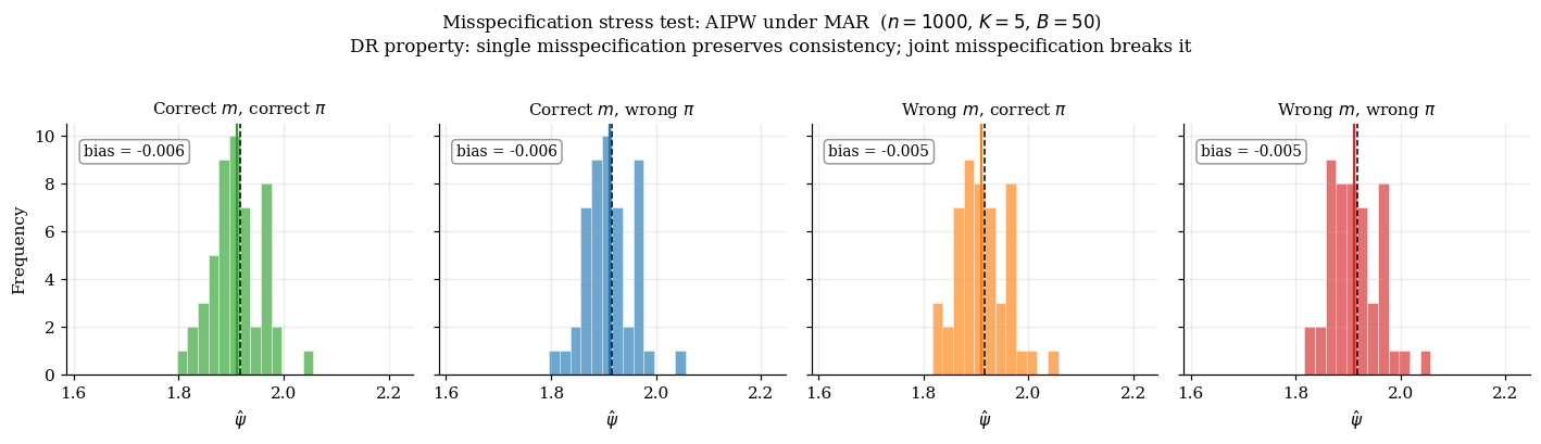
The DGP is the §3.4 MAR mean. The misspecifications:

• Correct $m$: OLS with features $(1, x_1, x_2, x_2^2, x_3)$ — contains the truth.
• Wrong $m$: OLS with features $(1, x_1, x_2, x_3)$ — omits $x_2^2$.
• Correct $\pi$: logistic with features $(1, x_1, x_2, x_3)$ — contains the truth.
• Wrong $\pi$: logistic with features $(1, x_1, x_2)$ — omits $x_3$.

Four scenarios. The double-robustness property predicts: any single misspecification leaves the AIPW estimator consistent. Only the (wrong, wrong) scenario should produce non-zero bias.

MC replications B: 80

13.4 The double-robustness consolation prize

Double robustness protects against single misspecification, not joint misspecification. When both nuisances are wrong — the default state of affairs when both are fitted with flexible ML on finite data — AIPW is biased.

The honest framing: double robustness is a consolation prize. The §7 rate condition is the more fundamental story: AIPW (and one-step / TMLE / DML generally) is asymptotically efficient when both nuisances converge faster than $n^{-1/4}$ to their respective truths, not to arbitrary limits.

Operational implications. Invest in better nuisance models. Cross-validate nuisance learners against each other on held-out data. Use ensemble methods. Treat double robustness as a backstop for when one model fails unexpectedly, not as a license to be lazy with both.

§14. Connections and limits

14.1 Forward-pointers retired

This topic was scoped around discharging six internal forward-pointers across five already-shipped formalML topics, plus one sister-site reciprocal:

• local-regression §12.1 (Robinson partial-linear with local-cubic nuisance) → realized in §9.2.
• high-dimensional-regression §12.1 (DML with debiased-lasso nuisance) → realized as a black-box rate citation in §7.3.
• causal-inference-methods (AIPW/TMLE worked examples generalized) → realized in §9.1 and §12.
• uncertainty-quantification §14.1 (EIF correction for variance functionals) → realized in §11.
• Sister-site reciprocal: formalStatistics: empirical-processes — discharged via the formalstatisticsPrereqs entry in this topic’s frontmatter.

14.2 The asymptotic regime — what the theorems do and don’t say

The §4.1 BKRW theorem, the §5.3 one-step asymptotic normality theorem, and the §7 DML CLT are all asymptotic statements. In finite samples, the asymptotic claims are approximations.

The notebook MC experiments at $n = 1000$ show: Wald 95% CIs cover at empirical rates of roughly 92–95% — within a few percentage points of nominal, but reliably below nominal at modest $n$. The empirical SD of cross-fit DML matches $\sqrt{V_{\rm eff}/n}$ to within ~10%, not exactly. The asymptotic normal approximation has detectable skewness in the bulk and especially in the tails.

These are not defects of the framework. The asymptotic theory is correctly applied; the finite-sample residuals are the natural consequence of working at $n = 1000$ with constants the asymptotics don’t capture. As $n$ grows, the gaps shrink.

14.3 The rate condition as a hypothesis

The §7.3 rate condition is the lever that makes everything work. It’s also the most consequential assumption in the topic, and the one most likely to fail silently.

Regimes where the rate condition holds with comfortable margin. Smooth regression functions in low-to-moderate dimensions ($d \leq 10$) with $n \geq 500$. High-dimensional sparse regression with $p \leq O(n)$. Parametric models that contain the truth.

Regimes where the rate condition fails or is uncertain. High-dimensional dense problems with $p$ comparable to or larger than $n$. Problems with discontinuous regression functions. Very-small-$n$ problems. Problems with extreme positivity violations.

The graceful failure mode. When the rate condition fails, the cross-fit DML estimator typically remains consistent (point estimate converges to the truth) but its inference (CIs, hypothesis tests) becomes unreliable. The point estimate is still informative; the SE is misleading.

14.4 Higher-order influence functions (deferred next layer)

When the §7.3 rate condition fails at the first-order level, a deeper construction sometimes works at the second-order level. Higher-order influence functions (HOIFs; Robins, Li, Tchetgen Tchetgen, van der Vaart 2008+) extend the EIF construction to capture not just the first-order von Mises term but also a second-order term that adjusts for the residual nuisance error. The resulting estimators have weaker rate-condition requirements — typically $o_P(n^{-1/(2k)})$ for the $k$-th-order estimator.

The cost: HOIF constructions are technically demanding, the second-order remainder requires its own analysis, and the resulting estimators are less well-tested in practice. For practitioners encountering rate-condition violations, the question is whether to invest in a better nuisance estimator (cheaper, more standard, often sufficient) or to switch to a HOIF construction (more complex, less tested, occasionally necessary). The right answer is typically the first.

Closing synthesis

The semiparametric inference framework gives us — in one unified construction — the abstract apparatus underneath modern flexible-nuisance estimation. The EIF $\phi^*$ is the central object: a function of an observation, derived by orthogonal projection in $L^2(P)$, that captures the per-observation contribution to the asymptotic variance of any RAL estimator. The BKRW theorem (§4) tells us $\|\phi^*\|^2$ is the lower bound on asymptotic variance. The one-step (§5), TMLE (§6), and DML (§7) constructions give us three concrete ways to hit the bound. The cross-fitting protocol (§8) extends the framework to ML nuisance under a $n^{-1/4}$-rate condition. The worked examples (§9) demonstrate the apparatus on canonical functionals. The inference machinery (§10) builds honest confidence statements. The connections (§11–§12) tie the framework back to uncertainty quantification and causal inference. The computational notes (§13) and limits (§14) close the topic with operational guidance and an honest accounting.

In one sentence: find the EIF, cross-fit the nuisance, average, sandwich-SE, Wald-CI — that’s the recipe, and the theory behind it is what the rest of this topic explained.