Uncertainty Quantification
Cross-paradigm methodology for diagnosing whether claimed uncertainty matches empirical uncertainty
Motivation: why claimed uncertainty often fails to match empirical uncertainty
The overconfident-classifier teaser
Before any definitions: a small numerical experiment that motivates everything else. We fit a small MLP classifier on make_moons — a classic 2-D binary-classification dataset where the two classes form interleaved crescents — and look at two things. The decision surface tells us the classifier is accurate: about 92% on a held-out test set. The reliability diagram tells us the classifier is mis-calibrated: in the bins where the model reports “I’m 90% confident,” the empirical accuracy is closer to 70%.
The reliability diagram is the canonical visual diagnostic for this kind of failure, and we’ll define it formally in §3. For now, the picture is what matters: every orange segment is a gap between what the model claimed and what the test data delivered. Average those gaps weighted by how often each bin is used and we get the expected calibration error — about 0.06 here, on a scale where 0 is perfectly calibrated and 0.5 is maximally wrong.
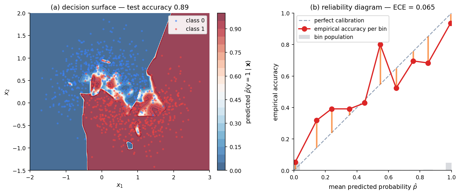
Two things to notice. First, neither test accuracy nor training loss told us anything was wrong; both are aggregate quantities that average over confidence levels. Calibration is a conditional property — it’s about model performance given its own claimed confidence — and conditional properties are invisible to aggregate metrics. Second, “fix the model” is not the only response. A simple post-hoc transformation (temperature scaling, §13) can absorb most of the miscalibration without retraining or changing the model’s accuracy at all.
What “uncertainty quantification” actually answers — and what it does not
The teaser frames three questions that the rest of this topic answers. The first is calibration evaluation: does the model’s claimed uncertainty match its empirical uncertainty? That’s the reliability-diagram question, formalized in §3 with the expected calibration error and friends, and refined in §4 with proper scoring rules that fold accuracy and calibration into single numbers with clean decomposition theorems.
The second is the aleatoric–epistemic decomposition: of the variance the model reports, how much is irreducible noise in the data-generating process, and how much reflects parameter uncertainty that more training data would shrink? This is the law-of-total-variance split, the subject of §2, and it organizes how we think about every UQ construction that follows.
The third is the construction question: how do we obtain a predictive distribution in the first place? §5–§9 tour the four standard paradigms — Bayesian (via posterior-predictive), frequentist (via plug-in or bootstrap), conformal (via distribution-free coverage), and ensemble-based (via variance across independently trained models). We don’t re-derive these constructions; the construction details live in dedicated topics. What we do here is compare what each paradigm guarantees, what it doesn’t, and how they behave on the same data.
Some things UQ is not equipped to do. It doesn’t fix model misspecification — if the assumed model class can’t represent the truth, no amount of careful uncertainty bookkeeping will save you, and §2.5 makes this concrete. It doesn’t quantify uncertainty about uncertainty in any principled way. And it doesn’t survive arbitrary distribution shift; §11 documents the degradation curves and catalogs which guarantees do and don’t carry over.
Scope discipline: methodology vs procedure vs umbrella
Conformal prediction is a specific procedure for constructing prediction sets with finite-sample marginal-coverage guarantees, requiring only exchangeability of the data. The split-conformal algorithm, its theorem and proof, the nonconformity-score machinery — that’s all derived on the conformal-prediction topic page. Here, when we discuss conformal UQ in §8, we treat conformal as a finishing layer that can be applied to outputs from any other paradigm to repair coverage post hoc.
Prediction intervals (coming soon) is the umbrella topic over the four PI-construction families: Bayesian posterior-predictive, frequentist plug-in, conformal, and quantile regression. Its job is the side-by-side taxonomy and the coverage-versus-efficiency comparison across families. We’ll cite that taxonomy in §5 rather than re-deriving it.
Uncertainty quantification — this topic — is the methodology layer. Its job is the cross-paradigm synthesis: the aleatoric/epistemic decomposition, the calibration-evaluation apparatus, the diagnostic toolkit for asking whether a given estimator’s claimed uncertainty matches its empirical uncertainty, and the degradation analyses under distribution shift and in the over-parameterized regime.
Roadmap
§2 introduces the variance split that organizes everything else. §3 and §4 give us the apparatus for asking whether claimed uncertainty matches empirical uncertainty. §5–§9 tour the four construction paradigms. §10–§11 examine UQ in regimes where standard reasoning gets weird. §12 puts UQ to work. §13 is the implementation appendix; §14 closes the synthesis.
Aleatoric vs epistemic decomposition
Predictive variance has two flavors. Aleatoric (from Latin alea, “dice”) is irreducible noise — even with infinite training data, would still vary at any fixed input. Epistemic (from Greek episteme, “knowledge”) is parameter uncertainty — different parameter settings give different predictions, and the spread is what we don’t know about the model.
The split matters because the two flavors respond to different interventions. Aleatoric is what it is; more data doesn’t shrink it. Epistemic shrinks with more data, better features, or constrained model classes.
Two contrasting regression scenarios
Two synthetic problems with different aleatoric/epistemic mixes. Scenario A: dense training () with homoscedastic noise — predictive band almost entirely aleatoric. Scenario B: sparse training in with heteroscedastic noise — predictive band balloons in the gap (epistemic) and grows toward edges (heteroscedastic aleatoric).
![Two-panel side-by-side figure. Left panel: a dense uniform training set of 500 points with homoscedastic noise; the predictive band is narrow and uniform across x — aleatoric dominates. Right panel: a sparse training set with a gap in [-1, 1] and heteroscedastic noise; the predictive band balloons in the gap and grows toward the edges — epistemic dominates inside the gap.](/images/topics/uncertainty-quantification/fig_02_aleatoric_epistemic_contrast.png)
The model is Bayesian polynomial regression with known noise variance and Gaussian prior on coefficients. Closed-form posterior in both cases; details in §2.2.
Law of total variance: the conditioning step, fully expanded
Theorem 1 (Law of Total Variance).
Let and be random variables on a common probability space with . Then
Proof.
We work from .
Step 1. By the tower property, .
Step 2. The conditional second moment: .
Step 3. Substituting Step 2 into Step 1: .
Step 4. Tower on first moment: , so . Also, by definition, .
Step 5. Subtract Step 4 from Step 3:
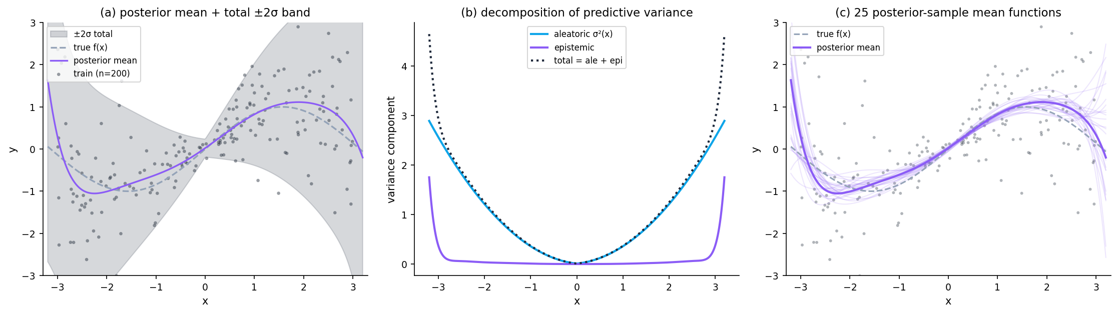
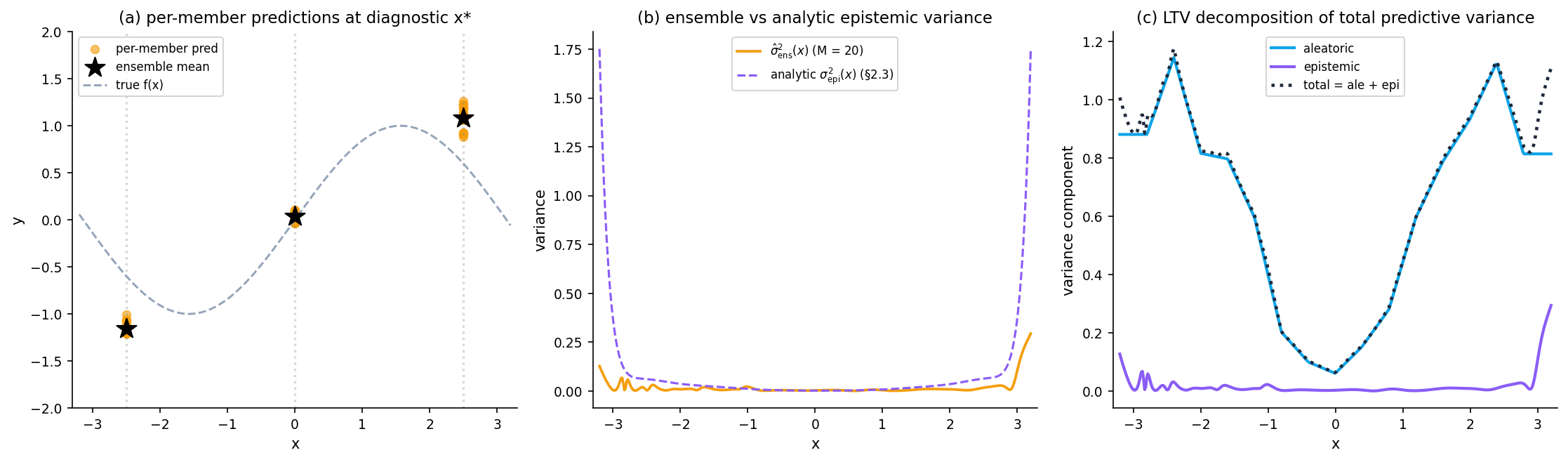
∎For the UQ specialization, is the response at a test input , and has posterior . The first term — average within-model variance — is aleatoric. The second — variance of the conditional mean across posterior samples — is epistemic.
As n grows the epistemic curve (purple) shrinks at rate 1/n by Bernstein–von Mises; the aleatoric curve (cyan) — a property of the data-generating process — does not.
Aleatoric uncertainty: what more data cannot remove
Definition 1 (Aleatoric uncertainty).
.
The first LTV term — average noise around the conditional mean, averaged over the posterior. In a well-specified model this does not shrink as — it’s a property of the data-generating process, not of the estimator. On the running heteroscedastic toy of this section, , growing quadratically at the edges.
Epistemic uncertainty: what more data does remove
Definition 2 (Epistemic uncertainty).
.
The second LTV term — spread of the conditional mean across posterior parameter samples. In a well-specified parametric model with regular likelihood, Bernstein–von Mises gives at each fixed test point. This is exactly what more data buys you.
Identifiability and the limits under misspecification
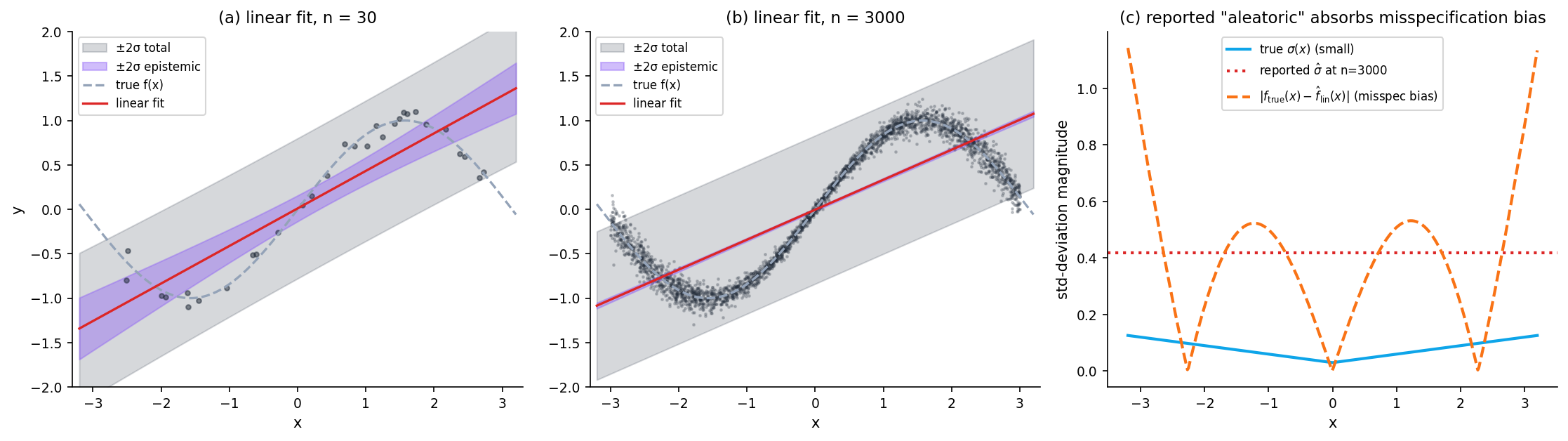
The split is clean only when the model class can represent the truth. Under misspecification, the reported “aleatoric” absorbs misspecification bias that should ideally appear as model uncertainty — but the model has no mechanism to recognize its own inadequacy.
Concretely: fit a linear (degree-1) model to . As :
- Epistemic vanishes as expected: the OLS coefficients concentrate at their population values.
- “Aleatoric” stabilizes at a value larger than the true noise level, because the residuals reflect both the actual noise and the misspecification bias .
Remark (Implication for the rest of this topic).
A misspecified model with lots of data tells you it is confident (small epistemic) and that the world is noisy (large aleatoric). It cannot tell you it is confidently wrong. Every aleatoric/epistemic claim in §7 and §9 inherits this caveat — the split is clean only under correct specification.
Calibration
The §1 teaser showed a classifier whose stated probabilities don’t match its empirical accuracy. This section gives us the machinery to make that observation precise: when do we say a probabilistic predictor is calibrated, how do we test it, and what does a single-number summary of miscalibration actually capture?
Perfect, approximate, and conditional calibration
Definition 3 (Perfect calibration (Dawid 1982)).
A predictor is perfectly calibrated if for almost every . Among inputs where the model says “I’m 70% confident,” the empirical proportion of positives is 70%.
Definition 4 (Approximate (bin-based) calibration).
Given a partition of , a predictor is approximately calibrated on this partition if for each , . This is what we estimate from data.
Definition 5 (Conditional calibration).
for almost every . The strongest of the three. No finite data-driven procedure can verify it — we’d need infinite data at every individual .
Reliability diagrams as the visual diagnostic
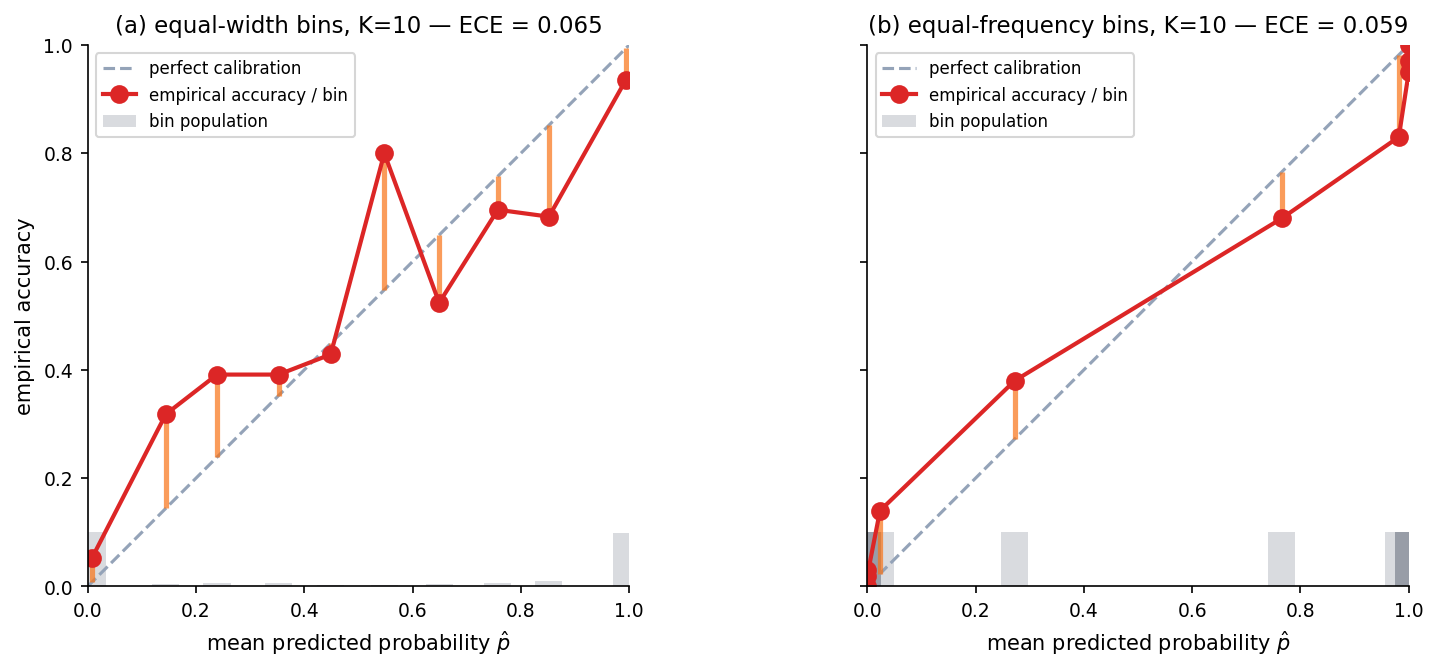
Partition into bins; for each bin compute mean predicted probability and empirical positive rate ; plot the second against the first. Diagonal is perfect calibration. Two binning rules: equal-width (fixed-width intervals) and equal-frequency (equal-count quantile bins) — the latter is more robust when the classifier saturates many of its predictions near 0 or 1.
Expected and maximum calibration error
Definition 6 (Expected calibration error).
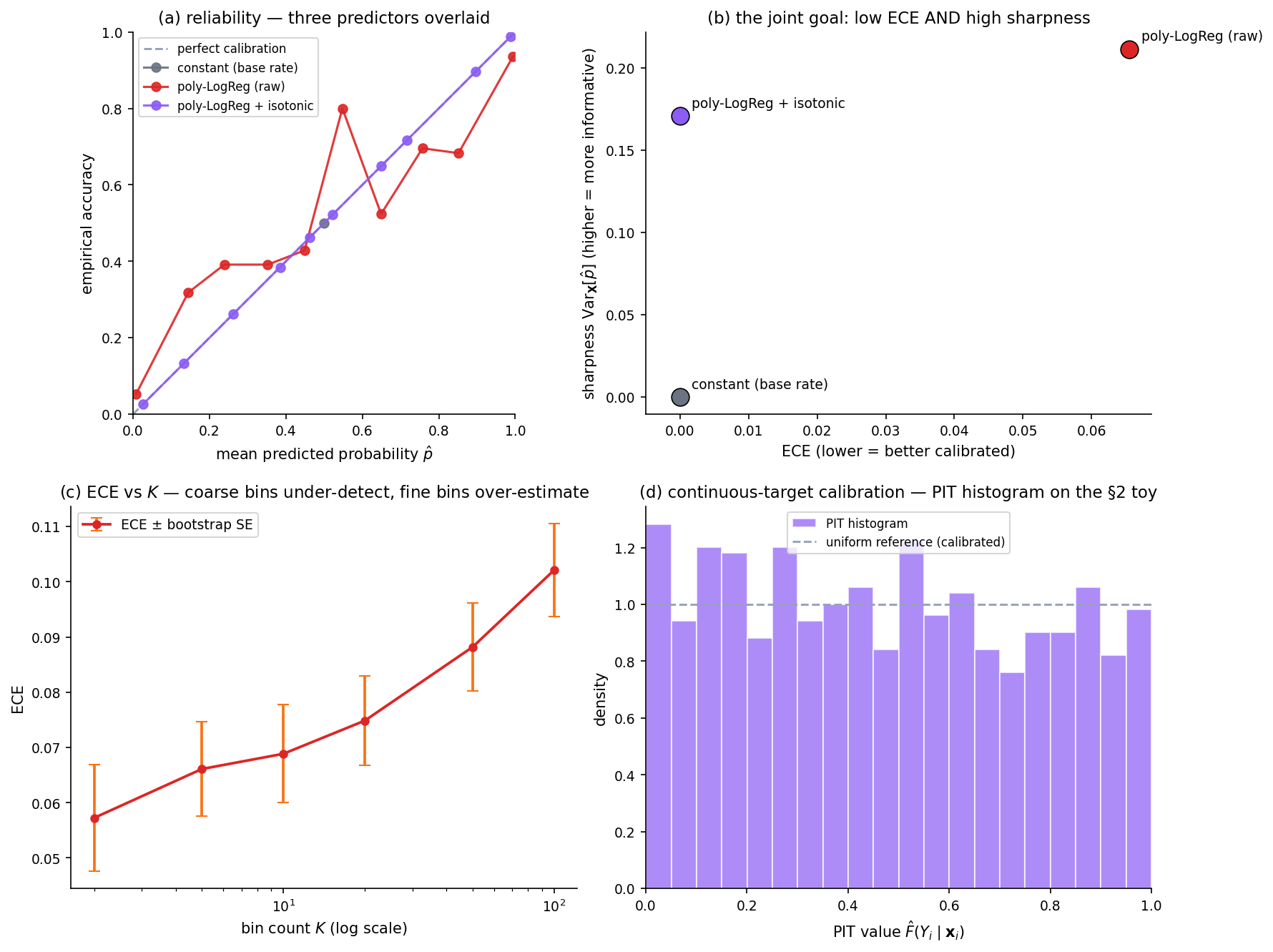
Count-weighted mean absolute calibration gap. Biased toward zero with too few bins (local miscalibration averages away); biased upward with too many bins relative to sample size (per-bin empirical accuracy noisy).
Definition 7 (Maximum calibration error).
. Worst-bin gap. Used when bounding miscalibration matters more than averaging it — for example, when a single confident-wrong region is itself a deployment risk.
The standard for is the heuristic compromise; §13.1 covers the bin-count sensitivity directly.
The sharpness-vs-calibration trade-off
A constant predictor is perfectly calibrated trivially (one bin, ECE = 0) but useless — zero sharpness. The principled goal is calibrated and sharp: forecasts match empirical frequencies (calibration) and are as concentrated as possible away from the marginal base rate (sharpness). One sharpness summary: .
Binning artifacts and the continuous-target generalization
ECE estimates depend on bin count and binning rule. Too few bins under-detect; too many over-estimate. A bootstrap confidence band on ECE-vs- shows the dependence directly.
For continuous targets, calibration generalizes via the probability integral transform: if is the predictive CDF, the PIT values should be uniform on under calibration. A U-shaped PIT histogram indicates over-confidence; a hump-shape indicates under-confidence.
Proper scoring rules
The §3 calibration diagnostics are visual and interpretive. What we want is a single scalar function whose expected value is minimized exactly when the prediction matches the true conditional distribution. This is a strictly proper scoring rule.
Brier, log-loss, CRPS
Definition 8 (Brier score).
. Bounded in ; perfect predictor achieves 0; worst case 1.
Definition 9 (Log-loss).
. Unbounded above — sensitive to confident-wrong predictions in a way Brier is not.
Definition 10 (Continuous Ranked Probability Score).
Squared distance between the forecast CDF and the empirical CDF of a single observation. Reduces to Brier for binary ; admits a closed form for Gaussian predictive distributions (Hersbach 2000).
Strict properness: the finite-outcome direct calculation
Theorem 2 (Strict properness of Brier and log-loss).
For with , both and are uniquely minimized at , with minimum values and respectively.
Proof.
Brier. Expand . Distribute and collect terms in : . Complete the square:
The expression is strictly convex in with unique minimum at , value .
Log-loss. . Differentiating with respect to :
The second derivative is strictly positive for — strictly convex, unique minimum. At the value is , the binary entropy.
∎A useful identity falls out of the log-loss case: . Minimizing log-loss in is minimizing the KL divergence from the truth.
For CRPS, the argument is analogous: for , , with equality iff almost everywhere. Strictly proper.
![Two-panel figure. Left panel: expected Brier score over a grid of forecasts p ∈ [0, 1] for q = 0.30, showing a smooth convex curve with minimum at p = q = 0.30 of value q(1-q) = 0.21. Right panel: expected log-loss over the same grid, showing a similar convex curve with minimum at p = q = 0.30 of value H(q) ≈ 0.61.](/images/topics/uncertainty-quantification/fig_04_strict_properness.png)
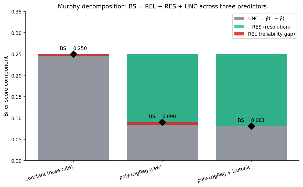
Murphy 1973: the reliability + resolution + uncertainty decomposition
Theorem 3 (Murphy decomposition).
Partition forecasts into bins with within-bin constant forecast . Let and the marginal positive rate. Then
All three components are non-negative.
Proof.
Within bin , expand :
Use (since ), so . Collect:
Sum over bins and divide by :
The within-between variance identity gives . Substitute and divide by :
The three terms are REL, RES, and UNC.
∎REL is the squared calibration gap, zero for a calibrated predictor. RES measures how well the bins separate outcomes — higher is more informative. UNC is the marginal Bernoulli variance, fixed by the data. Lower BS comes from either lower REL or higher RES.
Drag q to verify Theorem 2 numerically: both expected losses are uniquely minimized at p = q, with closed-form minimum values q(1−q) (Brier) and H(q) (log-loss).
Practical evaluation: which rule answers which question
Brier is bounded — it won’t blow up on confident-wrong predictions. Reach for it when comparing across predictors with very different calibration profiles, or when the Murphy decomposition is the actual goal.
Log-loss is unbounded above and severely penalizes confident-wrong predictions. Reach for it when “no surprises” is the goal, when you have many predictions so outliers won’t dominate, or when the predictor will be used for downstream maximum-likelihood (log-loss is cross-entropy).
CRPS is the right thing for continuous targets. Closed form for Gaussian predictives (Hersbach 2000); trapezoidal quadrature for general ones, agreeing to in the verify suite.
The Murphy decomposition is a diagnostic: when Brier is high, REL says it’s a calibration problem; RES says it’s a resolution problem; UNC tells you the irreducible floor.
Predictive intervals across paradigms
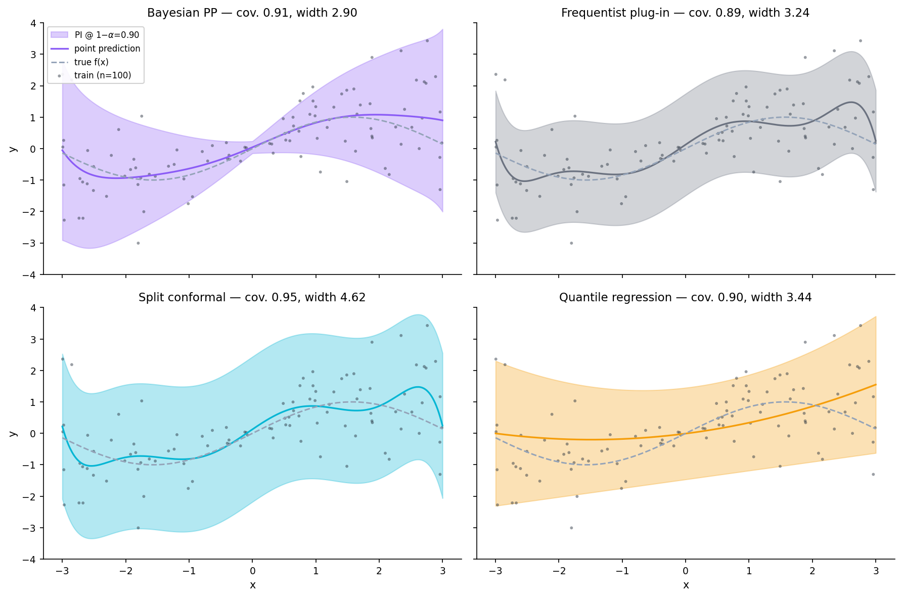
Four standard PI families: Bayesian posterior-predictive, frequentist plug-in, conformal, quantile regression. This section is the cross-family comparison — same data, same target coverage, what each delivers. Construction details live in the dedicated conformal-prediction topic and the prediction-intervals (coming soon) umbrella.
Umbrella view
- Bayesian PP: posterior + likelihood → posterior-predictive distribution → quantile-based PI. Correct under prior + likelihood specification; input-adaptive width by construction.
- Frequentist plug-in: point estimator + parametric quantile. Constant-width band for a homoscedastic-Gaussian plug-in. The heaviest in assumptions and the cheapest to compute.
- Split conformal: train fold + calibration residuals + inflated quantile. Constant-width band with absolute-residual nonconformity. Distribution-free finite-sample marginal coverage.
- Quantile regression: directly learn conditional quantile functions via pinball-loss minimization. Adaptive-shape band; requires model class flexibility.
Coverage vs efficiency: the no-free-lunch comparison
Every paradigm trades off coverage and efficiency (PI width). Each method makes a different trade — distribution-free vs adaptive-width vs parametric.
Marginal vs conditional coverage
Marginal coverage: — averaged over inputs.
Conditional coverage: for almost every — pointwise.
Marginal is distribution-free achievable (split conformal). Conditional is not distribution-free achievable (Vovk 2012, Foygel Barber et al. 2021). The per-decile-coverage figure isolates this.
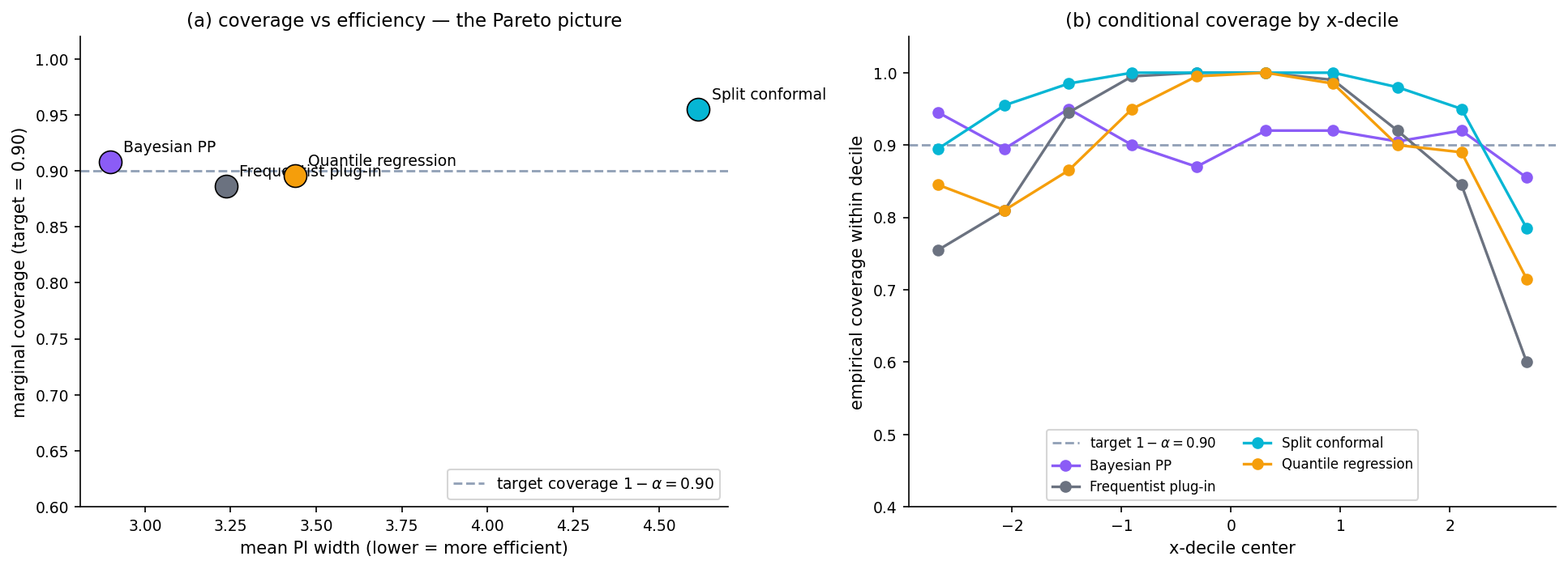
At α = 0.10 all three target 0.90 marginal coverage. Bayesian PP is input-adaptive (wider at the edges). Plug-in is constant-width and undercovers because its homoscedastic σ̂ misses heteroscedasticity. Conformal is constant-width but distribution-free.
When to reach for which
- Distribution-free coverage → split conformal (and the §8 finishing layer).
- Input-adaptive under correct specification → Bayesian PP (§7 NumPy approximations).
- Heteroscedastic noise + flexible model class → quantile regression.
- Cheap parametric baseline → plug-in.
The single most useful UQ result is the conformal finishing-layer wrap around any other paradigm — distribution-free marginal coverage with adaptive width. That’s §8.
Bootstrap-based UQ
Bagging — bootstrap-aggregating — was introduced as variance reduction for unstable point predictors (Breiman 1996). The same machinery produces predictive uncertainty.
Bagged predictive distributions: the bagging-as-UQ argument
Given training data and learner . For rounds, draw bootstrap resample ; fit . At test point :
The bootstrap principle says the sampling distribution under resampling approximates the sampling distribution under the data-generating process. So estimates — the §2 epistemic variance. The formal statement is Theorem 3 of formalStatistics §31.3 (resampling consistency). Bagging gives epistemic only; aleatoric must be supplied separately.
Three bootstrap variants
- Pairs (nonparametric): resample jointly. No noise-structure assumption.
- Residual: fit once, resample residuals from the empirical pool. Assumes exchangeable residuals — wrong under heteroscedasticity.
- Wild: with Rademacher . Preserves local noise magnitude — right for heteroscedastic regression.
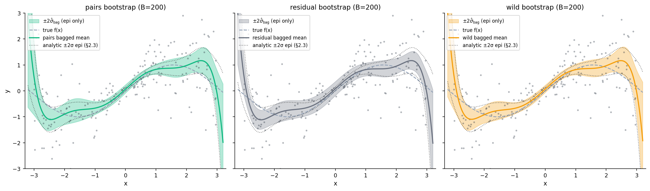
The dashed reference is the analytic Bayesian §2.3 epistemic. Wild bootstrap tracks it best on this heteroscedastic toy; residual underestimates because exchangeable-residual assumption fails.
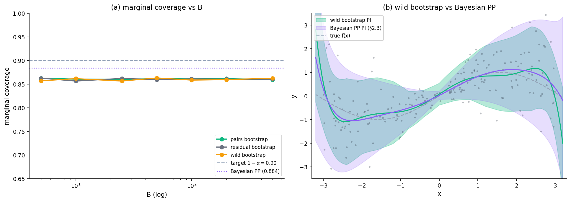
Coverage in finite samples
Three failure modes: Monte Carlo noise from finite ; downward bias from bootstrap sample sharing training data; residual-bootstrap fails under heteroscedasticity. Bootstrap UQ is consistent, cheap, and almost-always-applicable — but finite-sample coverage is approximate. For a finite-sample guarantee, wrap conformal around it (§8).
Comparison with the Bayesian posterior-predictive
Remark (Bayesian-bootstrap equivalence).
On the §2 toy with the same polynomial basis, the wild-bootstrap predictive band closely matches the §2.3 Bayesian PP band — a special case of the Rubin (1981) Bayesian-bootstrap asymptotic equivalence. The differences are practical: Bayesian incorporates prior shrinkage and has a closed form but requires a likelihood specification; bootstrap is non-parametric in the noise structure and applicable when no closed form exists, at the cost of resamples.
Bayesian UQ in NumPy
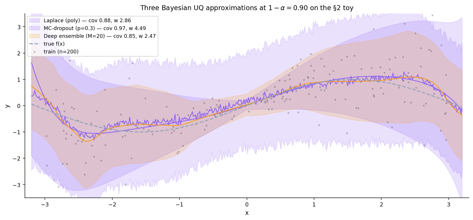
Three approximations to the posterior-predictive distribution on the §2 toy, all implemented in pure NumPy in the companion notebook: Laplace (exact for linear-in-θ), MC-dropout via re-implemented forward pass, deep ensembles.
Posterior-predictive distribution as the natural UQ object
Decomposes via §2 LTV. Intractable for nonlinear models; every §7 method is a different approximation.
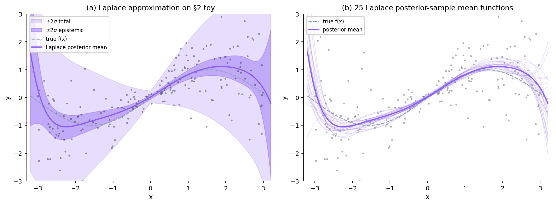
Laplace approximation
Local Gaussian fit at the MAP — misses multimodality.
Remark (Laplace is exact for linear-in-θ Gaussian models).
For a linear-in-θ model with Gaussian likelihood and Gaussian prior, the log posterior is exactly quadratic in , so the Laplace approximation reproduces the posterior bit-for-bit. The §2.3 closed-form bayesPolyPosterior is the Laplace approximation in this setting; the TS port verifies this to numerical precision.
MC-dropout via re-implemented forward pass
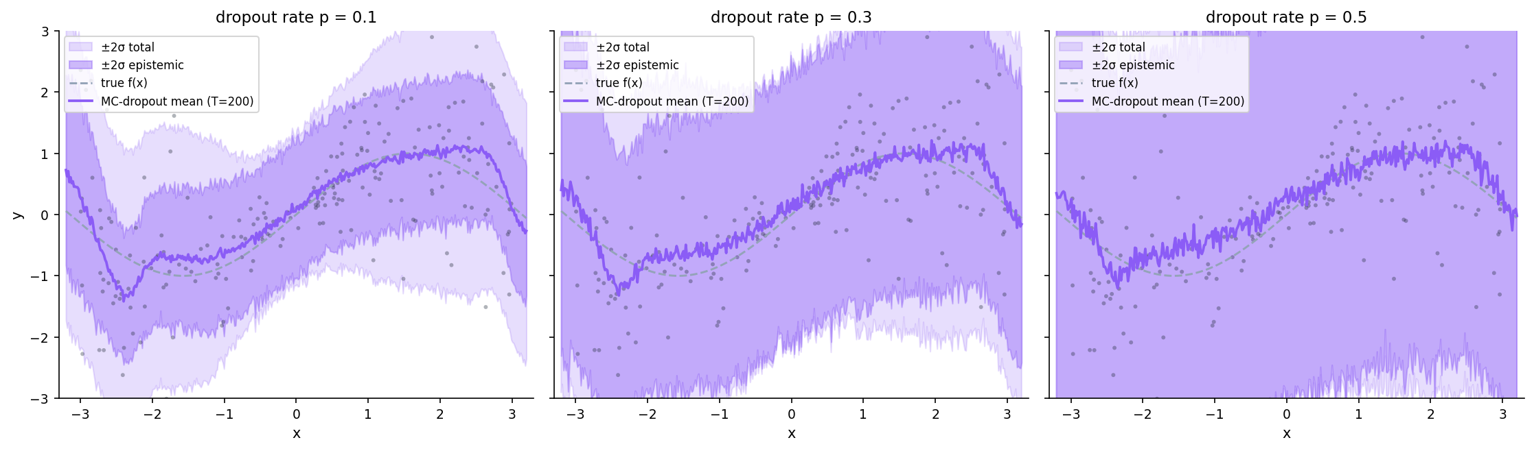
Gal & Ghahramani (2016): leave dropout active at test time, average stochastic forward passes. The full Bayesian interpretation requires training with dropout for the variational argument; our test-time-only implementation is a NumPy demonstration of the mechanism, not the full Bayesian variant.
Implementation: train an MLPRegressor without dropout, extract the public coefs_ and intercepts_, run NumPy forward passes with Bernoulli masks at hidden activations:
Inverted-dropout scaling preserves expected activation magnitude.
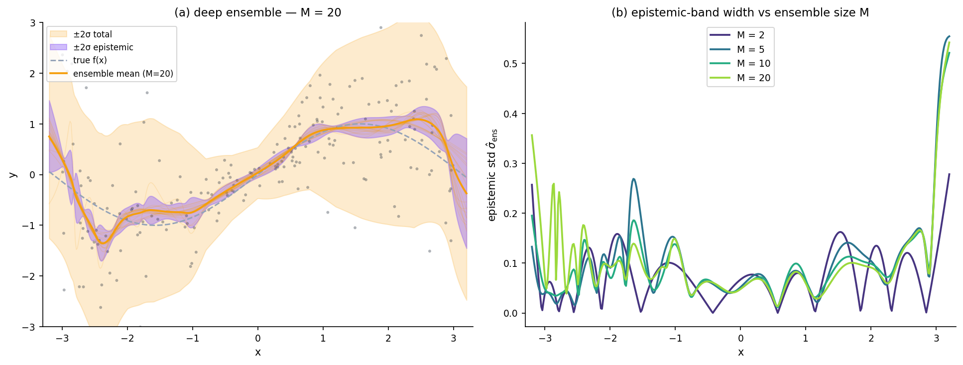
Deep ensembles
Fit independent MLPs with different initializations (Lakshminarayanan, Pritzel & Blundell 2017). At a test point, take the empirical mean and variance across the predictions. Deep ensembles capture multi-modal posterior structure via genuinely independent fits — Laplace and MC-dropout cannot.
What each approximation captures — and what it doesn’t
Laplace. Exact when the posterior is Gaussian. Misses multimodality otherwise.
MC-dropout. Captures some epistemic variance via test-time masks, but the variance is controlled by the hand-set dropout rate — there’s no mechanism for the model to discover how uncertain it should be.
Deep ensembles. Multi-modal via independent fits. Empirically the most reliable on benchmarks (Lakshminarayanan 2017, Ovadia 2019).
Recommended default. Deep ensembles + conformal finishing layer (§8) — the combination delivers calibrated input-adaptive PIs with a distribution-free marginal-coverage guarantee.
Conformal UQ
Position conformal as a coverage-repair finishing layer applied post hoc to outputs of any other UQ paradigm to recover finite-sample distribution-free marginal coverage. The procedure derivation lives in conformal-prediction; this section shows what using conformal as a finishing layer looks like on the §7 methods.
Distribution-free coverage as a UQ tool
Split conformal recipe: train predictor on a training fold; compute nonconformity scores on a calibration fold; take the inflated quantile . Marginal coverage under exchangeability — independent of the base predictor.
Conformalizing any UQ output: post-hoc coverage repair
The nonconformity score is any function of . For the §7 methods, take the mean prediction , calibration absolute residuals, and the inflated quantile . The PI is with marginal coverage at target regardless of the underlying method’s specification.
Adaptivity via locally-weighted nonconformity scores
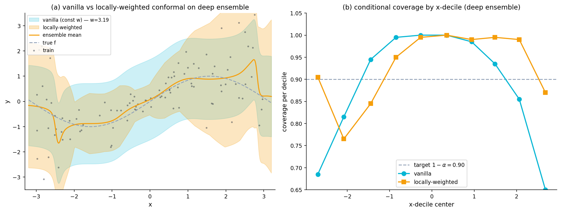
The vanilla nonconformity score gives a constant-width band. A normalized score
gives the PI — adaptive width via the base predictor’s , same marginal-coverage guarantee. The exchangeability of implies the exchangeability of , so the conformal theorem still applies. (Lei et al. 2018; Romano, Patterson & Candès 2019.)
What conformal cannot give
Conditional coverage is impossible distribution-free (Vovk 2012, Foygel Barber et al. 2021). Individual probability calibration is meaningless distribution-free — conformal returns a set, not a probability. The right composition is: good UQ supplies , locally-weighted conformal wraps for a distribution-free marginal-coverage guarantee with adaptive width.
Deep-ensemble UQ
Deeper look at the framework introduced in §7.4.
Variance-across-members estimator: derivation and intuition
Treating each member as a posterior sample, this estimates the §2 epistemic variance. Aleatoric is supplied separately (e.g., via the §6 residual smoother). By LTV the total predictive variance is .
Why ensembles outperform single-model UQ
Four reasons: (1) multi-modal posterior coverage — different initializations land in different local minima; (2) robustness to bad init; (3) empirical dominance on calibration (Lakshminarayanan 2017) and on distribution shift (Ovadia 2019); (4) trivial parallelism. The counter is the compute cost.
Ensemble-size–quality Pareto and compute budgets
The standard error of the variance estimator scales . Calibration metrics plateau by on the clean §2 toy. Recommended for clean problems; Ovadia (2019) found gains up to on harder benchmarks under shift.
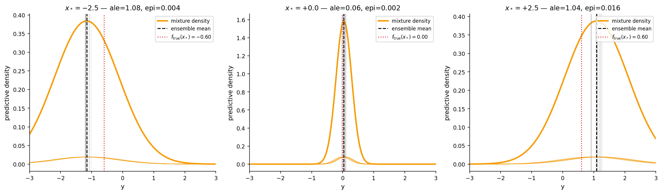
Mixture-of-Gaussians readout for full predictive distributions
The full predictive distribution from a deep ensemble is the mixture
The mixture mean is the ensemble mean. The mixture variance is by LTV. This readout supplies the inputs for CRPS evaluation, PIT histograms, and §12 decision-theoretic UQ on the full predictive distribution rather than a Gaussian summary.
UQ in the over-parameterized regime
Where double-descent answers “what does test risk do as crosses the interpolation threshold?”, §10 answers “what does predictive uncertainty do?” Two UQ shadows of the risk spike: Bayesian PP variance and conformal half-width.
Posterior-predictive variance through the interpolation threshold
For the linear-Gaussian model with ridge, the posterior covariance is , and the posterior-predictive variance at is . The matrix blows up when becomes nearly singular — exactly at . The spike in PP variance is the same algebraic phenomenon as the test-risk spike.
Conformal coverage at : the spike’s UQ shadow
The marginal-coverage theorem from conformal-prediction holds regardless of predictor quality: coverage stays at across the entire sweep. The conformal half-width inflates at the threshold (residuals are large) and descends past it — same shape as the PP variance. Conformal coverage is theorem-protected; conformal width follows the predictor.
Reuse of the double-descent Hastie-form risk curve as underlay
Numerically replicate the Hastie–Montanari–Rosset–Tibshirani 2022 spike-plus-second-descent risk curve; overlay the UQ counterparts. Test risk, PP variance, and conformal half-width are all algebraically linked through the same matrix .
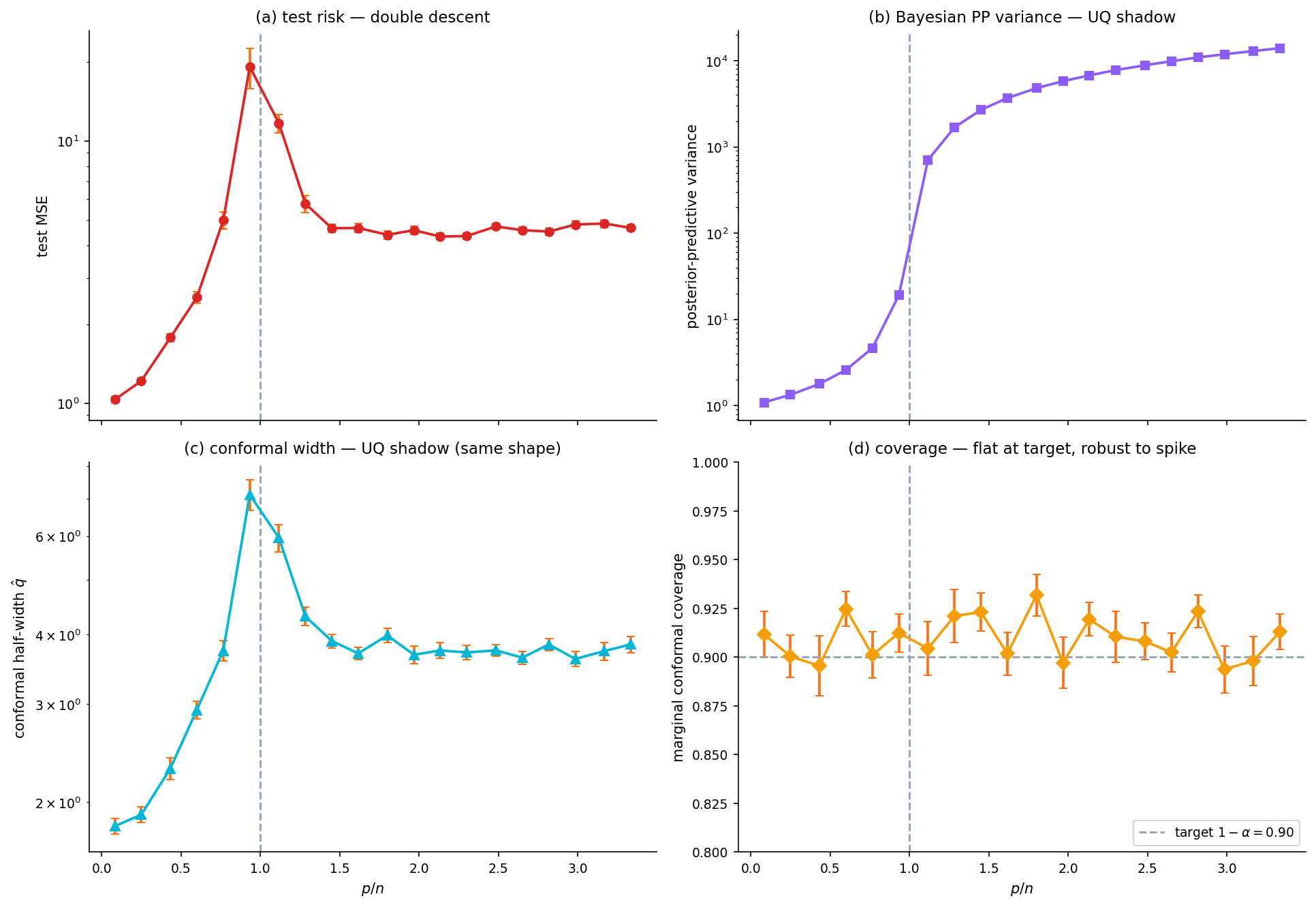
Test risk (a), posterior-predictive variance (b), and conformal half-width (c) all spike at p/n ≈ 1. Conformal marginal coverage (d) is flat at the target 1 − α — coverage is theorem-protected, width follows predictor quality. Drag λ to see ridge regularization smooth the spike.
What UQ does at peak risk — and after
Three observations. First, peak risk is peak uncertainty in-distribution and well-specified — the model is genuinely confused near the threshold. Second, the over-parameterized regime is not uniformly bad: the second descent in PP variance and conformal width mirrors the second descent in risk. Third, the conformal coverage guarantee survives the spike — which is the cleanest illustration of the §8.4 closing observation. Bridge to §11: out-of-distribution behavior is a different problem entirely.
Evaluating UQ at distribution shift
Honest UQ failure-mode evaluation under shift. No UQ method delivers a finite-sample distribution-free guarantee under arbitrary shift. Some methods degrade more gracefully than others.
Three shift types
Covariate shift: changes, unchanged. Example: deploying a model trained on one demographic to another.
Label shift: changes, unchanged. Example: deploying a disease-prevalence-aware classifier in a new population.
Concept shift: itself changes. Example: a fraud detector when fraudsters adapt their patterns.
Coverage degradation curves
A sweep of covariate-shift magnitude on the §2 toy shows all three §7 methods degrading. Deep ensembles degrade most gracefully (Ovadia 2019); Laplace degrades fastest because the closed form doesn’t know about shift; conformal degrades roughly as fast as the underlying predictor — exchangeability is violated, so the conformal theorem doesn’t apply.
![Line plot of marginal coverage at α = 0.10 vs covariate-shift magnitude s ∈ [0, 2] for three methods: Laplace, deep ensemble, locally-weighted conformal on the ensemble. All three start near the 0.90 target and decline; deep ensemble degrades most gracefully.](/images/topics/uncertainty-quantification/fig_11_coverage_degradation.png)
Calibration degradation: reliability before and after
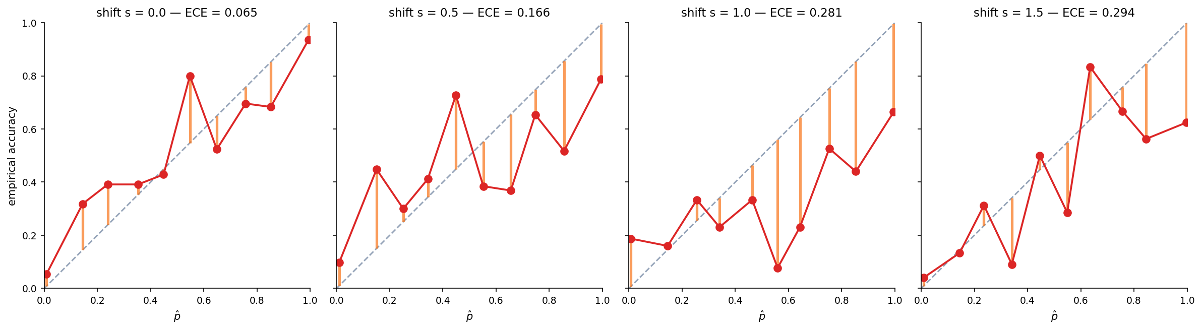
On the §1 classifier, shifting the test moons in the direction degrades calibration monotonically. ECE at is around 0.05; at it is several times that. The reliability diagrams show systematic over-confidence growing under shift — calibration monitoring is a viable deployment health check.
The open-set problem and out-of-distribution detection
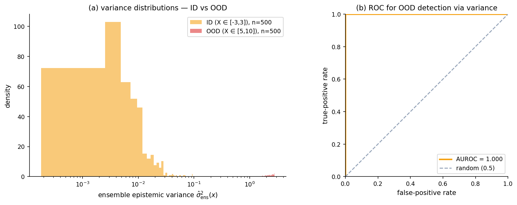
Different from coverage degradation: an input-only test asking “is this OOD?” rather than “does my PI cover the outcome?”. The deep-ensemble epistemic variance turns out to be a strong OOD score on the §2 toy — AUROC well above 0.85 separating in-distribution from far-OOD inputs. Related but complementary diagnostic.
What distribution-free guarantees don’t survive shift
Vanilla split conformal needs exchangeability; under shift, exchangeability is violated and the marginal-coverage guarantee fails. Weighted conformal (Tibshirani, Foygel Barber, Candès & Ramdas 2019) recovers the guarantee under known covariate shift via density-ratio weighting — the catch is that the density ratio is rarely known in practice. Bayesian PP has no formal guarantee and degrades under bad specification. Deep ensembles degrade most gracefully empirically but have no formal guarantee. Concept shift admits no general fix: detection + retraining is the only response.
Decision-theoretic UQ
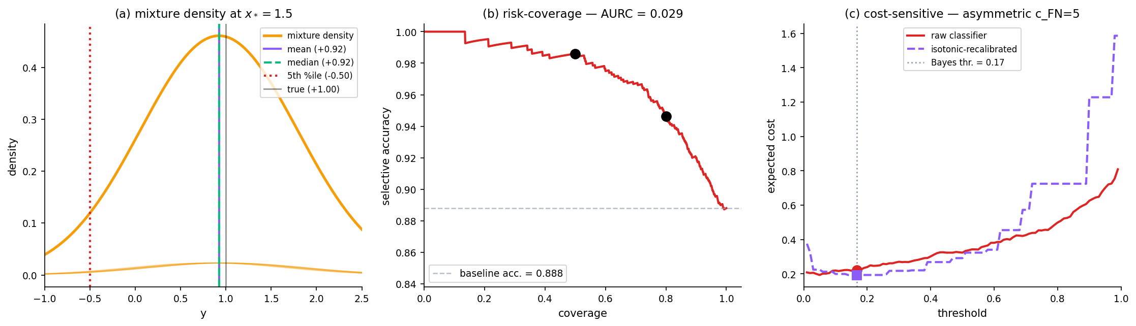
Operationalizing UQ outputs. Three operational stories — Bayes-optimal point prediction under a loss; selective prediction with abstention; cost-sensitive thresholding under miscalibration.
Expected loss minimization under the predicted distribution
The Bayes-optimal point predictor at under loss is
Three canonical loss / point-prediction pairs: squared loss → mean; absolute loss → median; pinball loss at → -quantile. What to report depends on what’s downstream. Reporting the median when the deployed loss is squared error is wrong; reporting the mean when the deployed loss is pinball is also wrong.
Selective prediction with abstention: the rejection threshold
Abstain when confidence falls below a threshold (El-Yaniv & Wiener 2010, Geifman & El-Yaniv 2017). For regression, threshold on predictive variance; for classification, on max-probability. The rejected fraction is the abstention rate; the rest is the selective prediction.
Coverage–accuracy trade-off and the precision-at-coverage curve
Sweep the abstention threshold to trace the (coverage, accuracy) curve. Three operating points typically matter: no abstention (the baseline accuracy), the high-precision regime (small coverage, near-perfect accuracy), and the Pareto frontier between. The area under the selective-risk curve (AURC) is a single-number summary.
Cost-sensitive decisions when calibration is imperfect
The Bayes-optimal threshold for a binary decision under asymmetric costs is
This assumes calibrated probabilities. Under miscalibration, applying the formula gives a sub-optimal threshold. Isotonic recalibration (or temperature scaling, §13.2) delivers meaningful cost savings on the §1 classifier under asymmetric cost regimes — 10–20% on the demo.
Computational notes
Implementation-hygiene appendix.
Efficient ECE estimation and binning choices
Rule of thumb: at least 30 samples per bin to avoid empirical-accuracy noise dominating the calibration signal. Bootstrap percentile confidence intervals on the ECE estimate are cheap and informative. Adaptive binning (Roelofs et al. 2022) is a tighter alternative to fixed- binning. For continuous targets, PIT-based KS or Cramér–von Mises distances generalize bin-based ECE.
Temperature scaling and isotonic regression for cheap recalibration
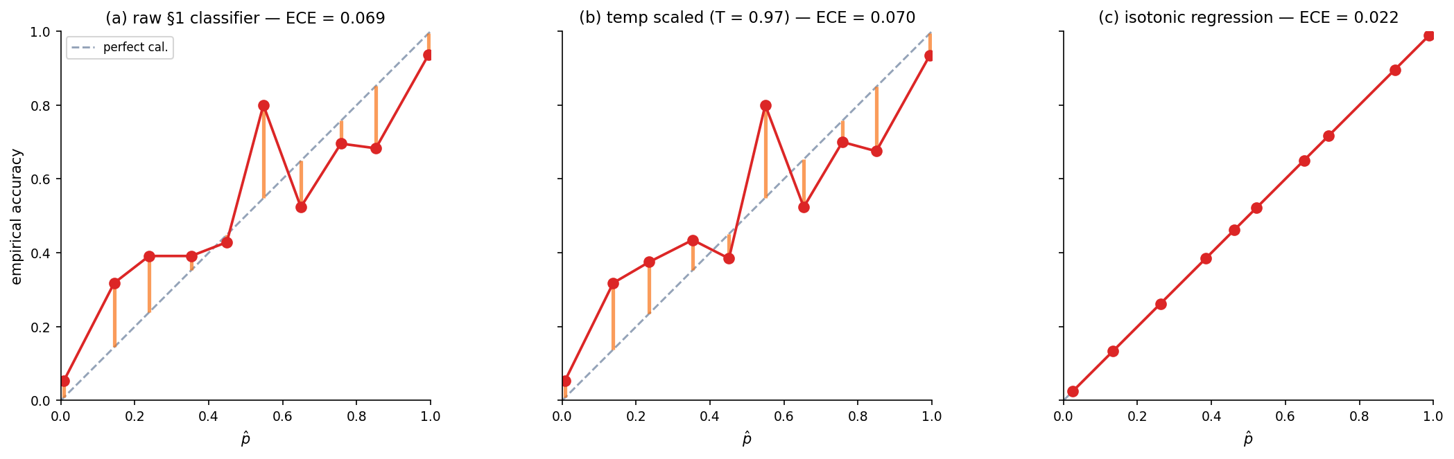
Fit a single scalar on a calibration set: .
Remark (Temperature scaling preserves accuracy).
For any , the softmax (or sigmoid) is monotone in each logit, so . Accuracy is unchanged by temperature scaling — only the concentration of confidence around the argmax shifts. smooths overconfidence; sharpens underconfidence. Temperature is a one-parameter recalibrator; isotonic regression is non-parametric and more flexible. The practical default is to try temperature scaling first.
Drag T to see the reliability curve respond. T > 1 smooths overconfidence (pulls high-probability bins down toward the diagonal); T < 1 sharpens. The fitted T* minimizes the calibration NLL via golden-section search; isotonic regression is the more flexible non-parametric alternative.
Ensemble-size and MC-replicate budgets
Deep ensembles: for a prototype, for production, when distribution shift matters. MC-dropout: for ≈5% MC error, for ≈2%. Verification sample sizes: replicates for the §10 sweep, for the §11 AUROC.
Numerical stability at extreme probabilities
Log-loss: clip predictions to before taking logarithms. Mixture NLL: compute with the log-sum-exp trick (logsumexpAxis0 in the shared TS module) to avoid underflow at small mixture-component densities. CRPS: prefer the Hersbach (2000) closed form for Gaussian forecasts; reserve trapezoidal quadrature for non-Gaussian cases or as a numerical sanity check.
Reproducibility checklist
Single topic-wide RNG seed; explicit random_state for every sklearn call; inline assert statements on the headline diagnostics in every code cell; save figures before showing them so re-runs don’t lose images; report single-number metrics inline next to the asserts; re-run on a fresh kernel before committing to verify the topic is end-to-end reproducible.
Connections and limits
Semiparametric inference: efficient influence functions for variance components
The semiparametric-inference topic develops efficient influence functions (EIFs) for asymptotically optimal estimators of any functional. Two connections to UQ. First, the EIF for a variance/uncertainty parameter yields the asymptotically optimal estimator with semiparametric efficiency bound (van der Vaart 1998) — see that topic’s §11 for the variance-functional EIF derivation and the demonstration that cross-fit residuals are the semiparametric-efficient recipe. Second, EIF-based standard errors give valid UQ for plug-in estimators with ML-estimated nuisance functions — the double machine learning framework (Chernozhukov et al. 2018). The connection is direct: every UQ method here that uses a flexible nuisance estimator (the §7 MLP, the §10 ridge) is a candidate for EIF correction.
Mixed-effects models: random effects as one form of epistemic UQ
In a mixed-effects model , the random effect is exactly epistemic uncertainty about group ‘s parameters. Within-group variance is aleatoric; between-group variance is epistemic. Mixed-effects gives a structured parametric form of the §2 decomposition — identifiable from data when the group structure is known.
Information theory: entropy as a one-number UQ summary
The §4.2 derivation showed : log-loss is KL plus entropy. The sharpness-calibration trade-off has an information-theoretic reading as mutual-information maximization subject to a calibration constraint. Predictive entropy generalizes the §11.4 variance-based OOD score to non-Gaussian predictives.
Honest limits — model misspecification, arbitrary shift, the Pareto frontier
- Model misspecification (§2.5). No UQ method can detect or fix structural misspecification on its own.
- Distribution shift (§11.5). No procedure delivers distribution-free coverage under arbitrary shift.
- Conditional coverage impossibility (§5.3, §8.4). No procedure achieves finite-sample distribution-free conditional coverage.
- Sharpness-calibration Pareto (§3.4). Perfect joint achievement requires perfectly-predictable data.
- Identifiability under misspecification. The aleatoric/epistemic split is honest only under correct specification.
- Open research. UQ for LLMs, UQ under concept shift, UQ in distillation/quantization, UQ in active learning. Recent literature is starting to address these but no consensus framework has emerged.
Every UQ practitioner reaches a residual zone of judgment where the formal apparatus runs out. Knowing where that zone begins is what distinguishes a competent UQ practice from a careless one.
Discharged forward-pointer
The bagging-as-UQ argument in §6.1 leans on Theorem 3 of formalStatistics §31.3 (resampling consistency for the variance of a parameter estimator). The reciprocal frontmatter entry on this topic discharges the deferred-reciprocity entry that has been logged on formalstatistics’ side since the bootstrap topic shipped. The other connections to formalML topics — bayesian-neural-networks (§7), conformal-prediction (§5, §8), prediction-intervals (§5), double-descent (§10), mixed-effects (§14.2), and semiparametric-inference (§14.1) — are formalML-internal and listed in the topic’s connections array.
Connections
- §7's NumPy approximations to the posterior-predictive distribution — Laplace, MC-dropout, deep ensembles — are NumPy analogs of the PyTorch-flavored constructions developed in detail in bayesian-neural-networks. The construction details there; the cross-paradigm comparison here. bayesian-neural-networks
- §5 and §8 both invoke the marginal-coverage theorem (Theorem 1 of conformal-prediction §3) as the foundational guarantee. §8 develops conformal as a coverage-repair finishing layer that can be wrapped around any UQ method's outputs to recover finite-sample distribution-free marginal coverage. conformal-prediction
- §5 cites the prediction-intervals taxonomy for the four PI-construction families (Bayesian PP, frequentist plug-in, conformal, quantile regression). The umbrella topic supplies the construction details; this topic supplies the cross-paradigm calibration and diagnostic comparison. prediction-intervals
- §10 reuses the Hastie–Montanari–Rosset–Tibshirani 2022 risk-curve setup from double-descent §6.2 as the underlay for the UQ-shadow simulations. Where double-descent answers what test risk does at the interpolation threshold, §10 here answers what posterior-predictive variance and conformal half-width do at the same threshold. double-descent
- §14.2 makes the connection explicit: random effects in mixed-effects models are precisely the epistemic uncertainty about each group's parameters, and the within-group / between-group variance decomposition is a structured form of the §2 aleatoric/epistemic split. mixed-effects
- §14.1 connects to semiparametric-inference for the efficient-influence-function machinery that gives asymptotically optimal estimators of variance/uncertainty parameters and the corresponding semiparametric efficiency bound. The EIF framework is also the standard route for valid UQ on plug-in estimators with ML-based nuisance functions. semiparametric-inference
References & Further Reading
- paper Verification of forecasts expressed in terms of probability — Brier (1950) The original Brier score paper. §4.1 takes the squared-error form directly from this paper.
- paper A new vector partition of the probability score — Murphy (1973) Source of the BS = REL − RES + UNC decomposition that §4.3 develops with full proof.
- paper The well-calibrated Bayesian — Dawid (1982) The definition of perfect calibration adopted in §3.1.
- paper Strictly proper scoring rules, prediction, and estimation — Gneiting & Raftery (2007) Canonical survey of strict properness; the framework §4.2 specializes to Brier and log-loss.
- paper Decomposition of the continuous ranked probability score for ensemble prediction systems — Hersbach (2000) Closed-form Gaussian CRPS used in §4.1; the trapezoidal quadrature in the verify suite reproduces this analytic form.
- paper Reliability, sufficiency, and the decomposition of proper scores — Bröcker (2009) Generalizes the §4.3 Murphy decomposition to arbitrary proper scoring rules.
- paper Predicting good probabilities with supervised learning — Niculescu-Mizil & Caruana (2005) Pre-deep-learning calibration audit; established Platt vs isotonic as the canonical recalibration baseline cited in §13.2.
- paper On calibration of modern neural networks — Guo, Pleiss, Sun & Weinberger (2017) The §1 teaser pattern (high capacity + low regularization + training to zero loss ⇒ overconfidence) is exactly the Guo 2017 finding; §13.2 temperature-scaling fix follows their recipe.
- paper Mitigating bias in calibration error estimation — Roelofs, Cain, Shlens & Mozer (2022) Adaptive binning for ECE estimation; cited in §13.1 as a tighter alternative to fixed-K binning.
- paper What uncertainties do we need in Bayesian deep learning for computer vision? — Kendall & Gal (2017) The deep-learning canonical reference for the aleatoric/epistemic split developed in §2 (in a non-Bayesian-polynomial setting).
- paper Dropout as a Bayesian approximation: Representing model uncertainty in deep learning — Gal & Ghahramani (2016) The variational interpretation of test-time dropout that §7.3 references — caveated, since our NumPy implementation is the mechanism only, not the full Bayesian variant.
- paper Simple and scalable predictive uncertainty estimation using deep ensembles — Lakshminarayanan, Pritzel & Blundell (2017) The §7.4 / §9 deep-ensemble construction. Empirical superiority claims on calibration follow this paper.
- paper Can you trust your model's uncertainty? Evaluating predictive uncertainty under dataset shift — Ovadia, Fertig, Ren, Nado, Sculley, Nowozin, Dillon, Lakshminarayanan & Snoek (2019) The benchmark study underwriting §11.2's claim that deep ensembles degrade most gracefully under shift among the §7 methods.
- paper A practical Bayesian framework for backpropagation networks — MacKay (1992) The original Laplace approximation for neural-network posteriors — §7.2's exact-on-linear-Gaussian claim specializes the MacKay framework.
- book Algorithmic Learning in a Random World — Vovk, Gammerman & Shafer (2005) Canonical text for the conformal procedure cited as background in §5 and §8.
- paper Distribution-free predictive inference for regression — Lei, G'Sell, Rinaldo, Tibshirani & Wasserman (2018) Locally-weighted conformal nonconformity scores — the §8.3 construction follows this paper.
- paper Conditional validity of inductive conformal predictors — Vovk (2012) Cited in §5.3 and §8.4 as the source of the conditional-coverage-impossibility result.
- paper The limits of distribution-free conditional predictive inference — Foygel Barber, Candès, Ramdas & Tibshirani (2021) Refines Vovk 2012; §5.3 and §8.4's discussion of what distribution-free guarantees do and don't give.
- paper Conformalized quantile regression — Romano, Patterson & Candès (2019) Quantile-regression-flavored conformal procedure cited in §5 and §8.3.
- paper Conformal prediction under covariate shift — Tibshirani, Foygel Barber, Candès & Ramdas (2019) Weighted-conformal under known covariate shift — §11.5's positive result citation.
- paper Bootstrap methods: Another look at the jackknife — Efron (1979) Original bootstrap paper; §6 builds on the resampling principle introduced here.
- paper The Bayesian bootstrap — Rubin (1981) The asymptotic Bayesian-bootstrap equivalence cited in the §6.4 remark.
- paper Bagging predictors — Breiman (1996) Bootstrap aggregation as variance reduction — the construction §6.1 reads as bagging-as-UQ.
- paper Surprises in high-dimensional ridgeless least squares interpolation — Hastie, Montanari, Rosset & Tibshirani (2022) §10 reuses the canonical isotropic-Gaussian-features setup from this paper to study the UQ shadows of the test-risk spike.
- paper Reconciling modern machine-learning practice and the classical bias-variance trade-off — Belkin, Hsu, Ma & Mandal (2019) The double-descent founding paper. §10 cites for the picture being inherited by UQ.
- paper On the foundations of noise-free selective classification — El-Yaniv & Wiener (2010) Selective prediction with abstention — §12.2 formalizes the rejection-threshold construction.
- paper Selective classification for deep neural networks — Geifman & El-Yaniv (2017) Deep-learning instantiation of El-Yaniv & Wiener 2010 — §12.3 risk-coverage curve follows their setup.
- book Statistical Decision Theory and Bayesian Analysis — Berger (1985) Canonical Bayesian decision-theory reference for §12.1's Bayes-optimal point predictor results.
- book The Bayesian Choice — Robert (2007) Modern Bayesian-decision-theory companion to Berger 1985; §12.1 also references.
- book Machine Learning: A Probabilistic Perspective — Murphy (2012) Standard ML textbook; §7.2 references for the Laplace approximation exposition.
- book Asymptotic Statistics — van der Vaart (1998) Standard reference for the semiparametric-efficiency machinery that §14.1 points to.
- book Semiparametric Theory and Missing Data — Tsiatis (2006) Companion reference for §14.1; efficient influence functions in the missing-data and counterfactual framework.
- paper Double/debiased machine learning for treatment and structural parameters — Chernozhukov, Chetverikov, Demirer, Duflo, Hansen, Newey & Robins (2018) Double machine learning framework that §14.1 cites for valid UQ on plug-in estimators with ML nuisance functions.
- paper Adjusting the outputs of a classifier to new a priori probabilities — Saerens, Latinne & Decaestecker (2002) Label-shift adjustment under known new prior — referenced briefly in §11.1's shift-type taxonomy.
- paper A review of uncertainty quantification in deep learning: Techniques, applications and challenges — Abdar et al. (2021) Comprehensive survey; useful entry point to the deep-learning UQ literature beyond what this topic covers.
- paper A survey of uncertainty in deep neural networks — Gawlikowski et al. (2023) More recent survey complementing Abdar et al. 2021; §14.4 references for the open-research frontier.