Generalized Method of Moments
Hansen's framework for over-identified estimation — efficient weighting, the J-statistic, and the bridge from ML to double machine learning
§1 — Introduction and motivation
Eighty-nine years separate Karl Pearson’s introduction of the method of moments in 1894 from Lars Peter Hansen’s generalization in 1982. In that span the field of statistics underwent the likelihood revolution, the rise of the Neyman–Pearson testing framework, and the bootstrap; econometrics absorbed all three and grew its own preoccupations on top. By the early 1980s rational-expectations models routinely produced more moment restrictions on a parameter vector than the parameter vector had components, and the just-identified inversion Pearson had relied on could no longer carry the load. Hansen’s resolution — minimize a weighted quadratic form in the sample-moment vector — is what we now call generalized method of moments (GMM). It earned Hansen a share of the 2013 Nobel Prize and has been the workhorse estimator of modern econometrics ever since.
We develop GMM from the just-identified Pearson setup forward, building the asymptotic theory, deriving the efficient weighting matrix and the Hansen J-statistic in full, and connecting GMM to maximum likelihood, instrumental variables, and the modern double machine learning of Chernozhukov et al. (2018). The reader should have seen Semiparametric Inference (the efficient-weighting matrix realizes the semiparametric bound), Convex Analysis (the GMM criterion is convex-quadratic in the moment residuals), and Concentration Inequalities (uniform laws of large numbers are the workhorse step in the consistency proof) before this topic.
1.1 From Pearson to Hansen — a century of moment matching
Pearson’s (1894) “Contributions to the mathematical theory of evolution” introduced the method of moments as a procedure for fitting a mixture of two Gaussians to a dataset of crab carapace measurements. The recipe was simple: compute the first sample moments, set them equal to the first population moments expressed as functions of , and solve the resulting system for . With equations in unknowns the problem was usually well-posed; Pearson did the arithmetic by hand for in the crab study, an order of difficulty that limited the method’s reach.
Then Fisher’s likelihood program subsumed nearly everything. From the 1920s through the 1960s the method of moments survived in textbooks as a pedagogical introduction to estimation, but in research it was sidelined as a “rough” alternative to maximum likelihood — asymptotically efficient only by accident, and noticeably inefficient in standard parametric families.
The setting that brought moment-based estimation back was rational-expectations macroeconomics. Hansen and Singleton’s “Generalized instrumental variables estimation of nonlinear rational expectations models” (1982, Econometrica) modeled a consumer’s Euler equation as
where is the discount factor, the coefficient of relative risk aversion, the gross asset return, and the agent’s information set at time . The conditional moment condition becomes a family of unconditional moment conditions — one for every -measurable instrument we choose — and as soon as we pick more than two instruments we have more equations than the two parameters to identify. The companion paper, Hansen’s “Large sample properties of generalized method of moments estimators” (1982, Econometrica), gave the framework that made this over-identified system into a well-defined estimator. Hansen shared the 2013 Nobel Prize for the asset-pricing applications of this machinery.
1.2 The over-identified problem — what L > k moment conditions break
Suppose we observe an i.i.d. sample from a distribution indexed by an unknown parameter . Economic theory — or a structural model, or a domain assumption — supplies a vector-valued moment function
such that the population moment condition
holds at the true parameter and at no other parameter in . The integer is the number of moment conditions; is the number of unknown parameters. Three regimes:
- Under-identified (): fewer equations than unknowns. Even in expectation the moment conditions do not pin down — the parameter is not identifiable from these moments alone, and no amount of data can rescue us.
- Just-identified (): as many equations as unknowns. The Pearson case. The system generically has a unique solution , and the sample-moment system generically has a unique solution that we can compute by inverting .
- Over-identified (): more equations than unknowns. In expectation the system is consistent — zeroes all moment conditions simultaneously by hypothesis — but in any finite sample has no solution at all. We have a redundancy of information that no choice of can absorb exactly.
The over-identified regime is the interesting one and the one Hansen’s framework targets. Why might we want more moment conditions than parameters? Because more conditions, even though they cannot all hold exactly in-sample, contain more information about than any subset of of them — and we want an estimator that uses all of them simultaneously rather than picking a subset and throwing the rest away.
Concrete prototype: linear instrumental variables. We posit a structural equation
where is endogenous (correlated with ) and is a vector of instruments assumed orthogonal to the structural error. The moment function is . With exactly, the unique solution to is the textbook IV estimator . With — more instruments than endogenous regressors — there is no that orthogonalizes the residual against every column of , and we need a principled rule for combining the moment conditions. That rule is GMM.
1.3 The GMM idea in one paragraph
The natural object to minimize is the magnitude of the sample-moment vector . But magnitude relative to what metric? Hansen’s framework parameterizes this freedom. Pick any positive-definite matrix — this is the weighting matrix — and define the GMM criterion
The GMM estimator corresponding to is the minimizer
Three facts make this work as a foundational estimation framework. First, any positive-definite delivers a consistent estimator: as , regardless of the choice of . Second, different choices of deliver different asymptotic variances, all of the same “sandwich” form, partially ordered by the Loewner ordering on positive-semidefinite matrices — and one specific choice uniquely minimizes the asymptotic variance: the inverse of the moment-residual variance , where . The resulting minimum-variance matches the semiparametric efficiency bound for the moment-condition model and gives Hansen’s framework its claim to optimality. Third, the value of the criterion at its efficient-weight minimum, , has an asymptotic distribution under correct specification — a free over-identification test that emerges as a by-product of the same quadratic form the estimator minimizes. Sections §4 through §8 develop these three facts in full.
1.4 Where GMM sits in the T6 track
GMM is the over-identified extension of formalStatistics: method-of-moments . That topic covers the just-identified Pearson case in detail; this topic picks up where Pearson stops, generalizing to and developing the asymptotic machinery the over-identified case requires.
Three formalML prerequisites carry direct weight. Concentration Inequalities supplies the uniform laws of large numbers that make the consistency proof go through: we need uniformly over , not just pointwise, and the empirical-process bounds from that topic are how we get there. Convex Analysis gives us the geometry of the criterion: is a positive-semidefinite quadratic form in , which means the criterion is convex in whenever is affine in (the linear case) and the first-order conditions are well-behaved more generally. Semiparametric Inference supplies the efficiency bound: the variance that efficient GMM achieves is the semiparametric efficiency bound for the moment-condition model, derivable from the efficient influence function of on the tangent space orthogonal to the moment-condition score.
Two formalML topics pick up where GMM leaves off. Causal Inference Methods (coming soon) extends to doubly-robust estimation, where the augmented inverse-probability-weighted estimator is GMM with a specific Neyman-orthogonal moment condition. The same topic covers double machine learning (Chernozhukov et al. 2018), where GMM-style score equations on first-stage nuisance functions produce second-stage point estimators whose asymptotic distribution is unaffected by the convergence rate of the machine-learned first-stage estimators.
§2 — Classical method of moments: the just-identified case
2.1 Sample moments and the moment equations
Given an i.i.d. sample from indexed by , Pearson’s construction picks scalar moment functions — a vector-valued — satisfying the population moment condition at the true parameter, and at no other parameter in . The method-of-moments estimator is the solution to the sample-moment equations
Two practical observations frame everything that follows. First, the choice of moment functions is a design choice: different functions give different estimators with different asymptotic variances, and the estimator is only as efficient as the moments are informative about . Second, in general the system has no closed-form solution, and we solve it numerically via Newton–Raphson or scipy.optimize.fsolve. The canonical illustrations below — Gaussian on the first two moments and Gamma on the first two moments — happen to admit clean closed forms; most nontrivial cases do not.
2.2 Worked examples — Gaussian and Gamma
Gaussian on . For with , the first two population moments are and . The MoM sample-moment equations are and , solved in closed form by and (the sample variance with divisor ).
For the Gaussian, this MoM estimator coincides exactly with maximum likelihood: the sufficient statistics for are precisely the first two sample moments, so the score equations reduce to the same system the MoM solves. We will see in §11 that every MLE is a just-identified GMM with the score equations as moment conditions; for the Gaussian, the first-two-moments MoM is also the score-equation MoM, and the two coincide.
Gamma on . For with density on , the mean is and the variance is . Equating to the sample mean and sample variance,
and solving gives the closed form
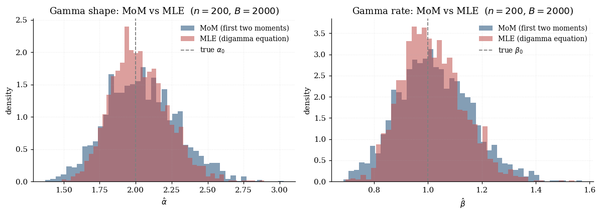
The MLE for the Gamma is not this estimator. The Gamma’s sufficient statistics are and , not and , and the MLE solves the digamma equation
where is the digamma function. This has no closed form; we solve it numerically. The MoM estimator on the Gamma is therefore consistent but not efficient — and the gap to MLE is large enough to see clearly at moderate sample sizes, as the visualization below demonstrates.
2.3 Asymptotic normality via the delta method
Theorem 2.1 (Just-identified MoM asymptotic normality).
Suppose , is twice continuously differentiable in in an open neighborhood of , the Jacobian
is non-singular, and is finite. Then
Proof.
The estimator solves . By the consistency assumption, lies in the smooth neighborhood for large enough. Taylor-expand each component around to first order, with the second-order remainder absorbed by a mean-value point on the segment between and :
where is the sample-Jacobian. The mean-value point varies by component, but the rest of the argument needs only , which follows from uniform LLN on over the neighborhood (a workhorse application of Concentration Inequalities) together with .
Rearrange and multiply by :
Two convergence facts complete the proof. By the central limit theorem applied to the i.i.d. observations with mean and covariance ,
By the continuous mapping theorem applied to matrix inversion (continuous at non-singular matrices), . Slutsky’s theorem combines these:
∎This is the just-identified case of the sandwich variance formula §5 will develop in full generality. With , the Jacobian is square and invertible by identification, so the “sandwich” collapses to the triple product . The weighting matrix does not appear because leaves no choice of how to combine moment conditions — the just-identified system has a unique solution.
A useful corollary: when the moment functions are the score, , the asymptotic variance reduces to the inverse Fisher information — the Cramér–Rao lower bound. To see this, note that under regularity (the negative Hessian of the log-likelihood in expectation), and (the information matrix equality). So . Choosing the score as moment function gives MLE efficiency; any other choice gives a consistent estimator with a (weakly) larger asymptotic variance in the Loewner ordering. This is why MoM on the Gaussian (where the first-two-moments are sufficient) matches MLE, and MoM on the Gamma (where the first-two-moments are not sufficient) does not.
2.4 Why we need GMM — over-identification kills direct inversion
What happens if we add a third moment condition to the Gaussian setup? Take
The third and fourth components exploit the Gaussian’s symmetry and the closed form for its fourth central moment (). In population all four moment conditions hold at . In any finite sample, however, the sample third central moment fluctuates around zero at rate and the sample fourth central moment fluctuates around at the same rate. So the system has no solution at finite : the first two equations pin down , and the third and fourth equations evaluated at that solution leave residuals of order .
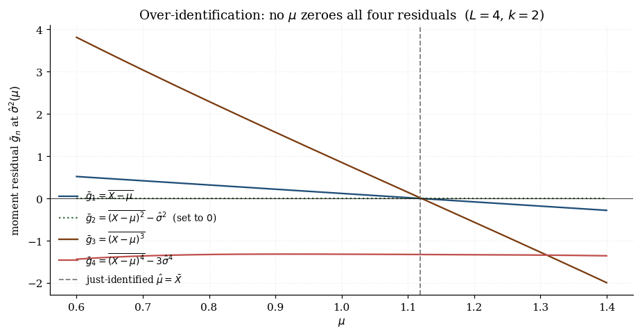
Three responses to this redundancy. We can drop two moment conditions and revert to a just-identified system — but which two, and why throw away information theory has supplied? We can use the first two to estimate and use the residuals in the third and fourth as a test of correct specification — a quick precursor to the Hansen J-statistic of §8. Or we can combine all four moment conditions through a positive-definite weighting matrix that absorbs their relative noise levels and trades off between them. This is GMM, and §3 develops it.
§3 — The GMM framework: moment conditions and weighted quadratic forms
This is the central definitional section. We formalize the over-identified moment-condition model, define the GMM criterion as a weighted quadratic form in the sample-moment vector, derive the first-order conditions that the GMM estimator solves, and lay out the rank condition that makes the whole construction work. Hansen’s (1982) original paper develops all four pieces in roughly five pages of dense notation; we expand them with concrete geometry and a worked running example.
3.1 Moment conditions and population identification
The GMM data-generating model has three pieces.
-
Sample. An i.i.d. sample from a distribution on a measurable space .
-
Parameter. An unknown , with an open subset of Euclidean space. (Compactness is sometimes imposed for the consistency proof in §4; we relax it where the geometry allows.)
-
Moment function. A known map , measurable in its first argument and continuously differentiable in its second, satisfying the population moment condition
The integer is the number of moment conditions; is the number of unknown parameters. We assume throughout. When we recover the just-identified Pearson setup of §2; the over-identified case is the one Hansen 1982 targets and the one this topic is about.
The moment condition is an identifying restriction: we further assume the population moment satisfies if and only if . Without this global identification hypothesis the population objective the GMM estimator targets has multiple zeros and consistency fails outright.
Running example. Throughout this section we use a synthetic problem that strips IV and endogeneity away and isolates the over-identified structure. We observe four scalar measurements at each , and on theoretical grounds we know the population means satisfy
With four measurements and two unknown parameters (, ), the system is over-identified. The moment function is
This is generalized-least-squares-via-moments — the simplest nontrivial over-identified GMM problem. The linear setup makes everything in §3 concrete and the criterion surface in §3.2 literally elliptical. §9 will replace the synthetic design with a structural instrumental variables setup.
3.2 The GMM criterion function
The sample moment vector is the empirical analog of ,
By LLN, pointwise (we will need uniform convergence for the consistency proof in §4, but pointwise convergence suffices to define the estimator). For the running example, where .
The GMM criterion function measures the magnitude of relative to a positive-definite weighting matrix :
where is symmetric and positive-definite. The factor of standardizes the criterion to an scale at : without it, and the asymptotic theory would be awkward. With the factor, converges in distribution (§8 gives the limit at the efficient weighting, and the analogous quadratic-form-in-Gaussians limit in general).
The criterion is non-negative, and equals zero only when . In the over-identified case (), for all at finite — the system has no solution that zeroes all residuals simultaneously — so the minimization
is a genuine minimization rather than root-finding. The minimum value is the residual GMM criterion — the unavoidable mismatch the over-identified system leaves behind, which §8 will repurpose as a specification test.
When is affine in , as in the running example, is exactly quadratic in :
Its contours in -space are concentric ellipses centered at , with shape controlled by and eccentricity reflecting how the four moment conditions trade off against each other under the metric .
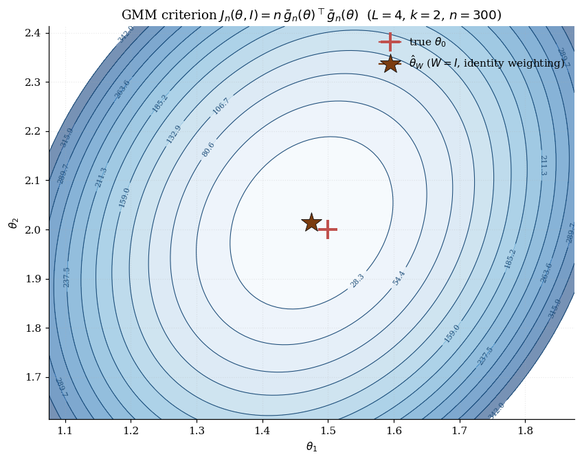
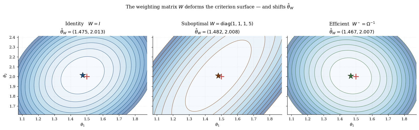
For general nonlinear , is convex in a neighborhood of — its Hessian at is , which is positive-definite under the rank condition in §3.4 — but may be non-convex globally. Practical optimization uses Newton–Raphson, quasi-Newton, or scipy.optimize.minimize; §13 covers the tips and traps.
3.3 First-order conditions — the GMM normal equations
Differentiate with respect to :
where is the sample Jacobian. Setting this to zero gives the GMM normal equations:
This is the over-identified analog of the just-identified system from §2. In the just-identified case (), is and generically invertible, so if and only if — the weighting matrix drops out and we recover the unique just-identified solution. In the over-identified case (), the system reduces from equations to equations through left-multiplication by , projecting the -dimensional moment residual onto the -dimensional column space of . The geometric reading is set the projection of the moment residual onto the parameter-direction subspace (in the metric ) to zero — we cannot zero the full -dimensional residual at any , but we can zero its projection along the directions that matter for .
For affine , the GMM normal equations have a closed-form solution. The running example gives (independent of ), so
This is generalized least squares, with the role of the GLS weighting matrix played by the GMM weighting matrix . For we get ordinary least squares of on ; for we get weighted least squares with variance-inverse weights; for the efficient choice where is the full moment-covariance matrix (off-diagonal terms included), we get the Aitken / Gauss–Markov estimator that achieves the smallest asymptotic variance. §6 derives this efficient choice.
3.4 Identification rank conditions
The GMM estimator is well-defined and the asymptotic theory works only if the model identifies . Two layers.
Global identification. The population moment has a unique zero at :
This is a hypothesis on the model — we assume it. For affine of the form , global identification reduces to having full column rank : equivalently being invertible. Geometrically, the columns of must span a -dimensional subspace of , so no two parameter vectors map to the same population mean vector.
Local identification — the rank condition. The Jacobian at the truth,
has full column rank :
This is the rank condition of GMM, and it carries three consequences we will rely on throughout the rest of the topic.
- The Hessian of the population criterion at is , positive-definite under the rank condition — so is a strict local minimum of the population objective.
- The sandwich variance that §5 derives is well-defined (the “bread” is invertible).
- The efficient-weighting variance that §6 derives is well-defined.
For the running example, has rank 2 iff the columns of are linearly independent. With the given the first two rows already form a identity submatrix, so the rank condition holds. The visualization below lets you watch the criterion surface degenerate as the design matrix is artificially collapsed toward rank deficiency.
What can go wrong? If the four moment conditions were with for all , every row of would be a scalar multiple of — has rank 1, is not identified by these moments (only the linear combination is), and no amount of data rescues the estimator. The model is under-identified despite having moment conditions. Over-identification counts equations, not information; the rank condition counts information.
When the rank condition holds exactly but is nearly rank-deficient — the columns of are nearly collinear in the metric — we have weakly-identified parameters (in the IV setting, weak instruments). The asymptotic theory still goes through but the asymptotic-normal approximation deteriorates at finite samples, and standard errors can be wildly understated. §9 covers the diagnostics for this case (the Staiger–Stock F-statistic for linear IV, the Anderson–Rubin test as a weak-instrument-robust alternative).
§4 — Consistency of GMM estimators
We turn to the first asymptotic result: as , the GMM estimator converges in probability to the true parameter . The result is almost free in the sense that it requires no particular choice of weighting matrix — any positive-definite limiting delivers consistency — and depends only on global identification plus a uniform law of large numbers on the sample-moment vector. What does require care is the bridge from pointwise convergence of at each to uniform convergence over , which is what the consistency proof actually needs. The technical workhorse is the empirical-process machinery developed in Concentration Inequalities.
4.1 Uniform laws of large numbers
The ordinary LLN gives us for each fixed — pointwise convergence. But the GMM estimator is the argmin of a function of , and pointwise convergence of the integrand is not enough to conclude that the argmin converges. A small pathological dip of far from can fool the optimizer even when each is close to in expectation; what we need is that no such dip happens anywhere in .
A function class obeys the uniform law of large numbers if
Two standard conditions, both inherited from Concentration Inequalities, deliver this. The bracketing-entropy condition asks that be compact, be continuous in for -a.e. , and a dominating function exist with and . This is the textbook Newey–McFadden setup (1994, Lemma 2.4); it gives convergence with no explicit rate. The Rademacher complexity condition asks that the class have Rademacher complexity that vanishes with . This gives an explicit rate — at the parametric when is VC or has bounded entropy.
For the linear running example , the function class is affine in parameters, has VC-dimension , and the uniform LLN holds at the optimal parametric rate . The connection to Concentration Inequalities is direct: the uniform LLN follows from concentration of the empirical-process supremum , controlled by Talagrand’s inequality, the bounded-differences inequality, or Massart’s symmetrization argument applied to the function class .
4.2 The population objective and global identification
Define the population criterion as the limit of :
Two properties drive consistency. First, for all , with equality iff ; this follows from positive-definiteness of . Second, under the global-identification hypothesis , the population criterion has a unique minimizer at , where .
Combining: uniquely. Consistency reduces to verifying that the sample argmin converges to the population argmin — a question for the argmax theorem (the consistency lemma for extremum estimators). The sample criterion is the empirical version of , scaled by : . The factor of does not move the argmin.
4.3 The consistency theorem
Theorem 4.1 (Consistency of GMM).
Assume (i) i.i.d. sample; (ii) compact parameter space ; (iii) global identification (); (iv) continuity of on for -a.e. ; (v) dominating function ; (vi) weighting with symmetric positive-definite deterministic. Then
Proof.
Four steps.
Step 1: uniform LLN. By (i), (iv), (v), the class satisfies the bracketing-entropy condition and the uniform LLN holds: .
Step 2: uniform convergence of the criterion. We show . Using the symmetric- identity ,
Take operator-norm bounds, sup over , and apply Slutsky with Step 1’s uniform LLN and assumption (vi). Result: .
Step 3: identification. By (iii) and positive-definiteness of , with equality iff . So is the unique minimizer of on .
Step 4: argmin convergence. Fix and let . By compactness of and continuity of , . On the failure event , the argmin definition and Step 2 give . So , which holds with probability going to zero by Step 2. .
∎(Originally Hansen 1982; the textbook treatment with these regularity conditions follows Newey & McFadden 1994 §2.) The proof carries a useful geometric reading. The sample criterion tracks the population criterion uniformly; the population criterion has a strict global minimum at separated by a positive gap from any point outside the -neighborhood; therefore the sample minimizer must eventually fall inside the -neighborhood. Compactness of guarantees the positive gap; the uniform LLN guarantees the sample criterion tracks the population criterion everywhere on , not just near the truth.
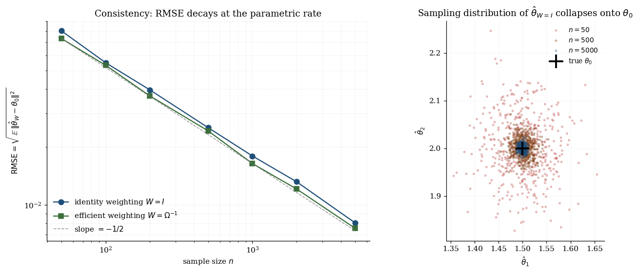
Two consequences worth noting before §5. Robustness to the weighting matrix. Theorem 4.1 imposes no special structure on beyond positive-definiteness — any positive-definite limiting weighting matrix gives a consistent estimator. The first-step identity-weight GMM and the second-step efficient -weighted GMM are both consistent. The proof template generalizes. The four-step proof — uniform LLN on the integrand, uniform convergence of the criterion, identification of the population minimizer, argmin convergence — is the template for proving consistency of every extremum estimator in statistics: MLE, M-estimators, GEL, sieve estimators, neural-network ERM. GMM is the prototype.
4.4 What can go wrong
Four failure modes, each illustrating which assumption above is doing the work.
Global identification failure. If the population moment has multiple solutions, is not the unique minimizer of — assumption (iii) breaks. The sample criterion has multiple local minima of comparable depth, and the argmin is not a well-defined limit object. Mitigation: re-parametrize to break the symmetry, or use a sign-restricted optimizer.
Rank deficiency. If has rank , the population criterion is flat along the null direction of near . The sample criterion inherits a near-flat ridge, the argmin is non-unique up to motion along the ridge, and the asymptotic variance in §5 blows up.
Weak identification. has full column rank but is nearly rank-deficient. Consistency still holds in principle (Theorem 4.1 applies — the rank condition is local-identification, not consistency), but the rate of convergence is governed by . At finite samples, the consistency-implied Gaussian approximation breaks down — the sampling distribution has heavy tails and CI coverage drops. §9.4 develops the linear-IV special case.
Dependent data. For non-i.i.d. data — time series, clustered samples — the LLN still applies under standard mixing or ergodicity conditions, but the moment-covariance in §5 must account for autocorrelation (HAC / Newey–West estimators replace the simple sample covariance). Consistency direction (Theorem 4.1) carries over with minimal modification; the asymptotic variance does not.
§5 — Asymptotic normality of GMM estimators
§4 established that . We now refine that result with the rate and limit distribution: , where is the sandwich variance that gives Hansen’s framework its characteristic asymptotic structure. Three ingredients — the Jacobian , the weighting matrix , and the moment-covariance — enter the formula, and reading their interactions sets up the efficient-weighting choice of §6 and the J-statistic of §8.
5.1 The sandwich variance formula
Theorem 5.1 (Asymptotic normality of GMM).
In addition to the consistency conditions of Theorem 4.1, assume (vii) lies in the interior of ; (viii) and is positive-definite; (ix) is continuously differentiable on a neighborhood for -a.e. , with a Jacobian uniform LLN and dominating function; (x) has full column rank . Then
The factor is the bread; the factor is the meat. The bread appears twice (once on each side of the meat) because the GMM normal equations are obtained by left-multiplying the moment residual by , so the inverse Hessian of the criterion enters the variance once for each application.
Two special cases collapse the sandwich. In the just-identified case (), is and invertible by (x). Algebraic cancellation gives — the weighting matrix drops out, recovering the §2.3 just-identified-MoM variance. Under efficient weighting (), the sandwich collapses to . §6 will show this is the Loewner-minimum of over all positive-definite — Hansen’s efficiency bound.
5.2 Proof via Taylor expansion of the first-order conditions
Proof.
The GMM estimator satisfies the first-order conditions . By consistency, lies in the differentiability neighborhood eventually. Five steps complete the argument.
Step 1 — mean-value expansion. By the mean-value theorem applied component-wise to ,
where lies on the segment from to .
Step 2 — substitute into the FOCs. This gives , where .
Step 3 — matrix convergence. By consistency, the Jacobian uniform LLN, and continuous mapping, . The rank condition (x) makes this invertible, so .
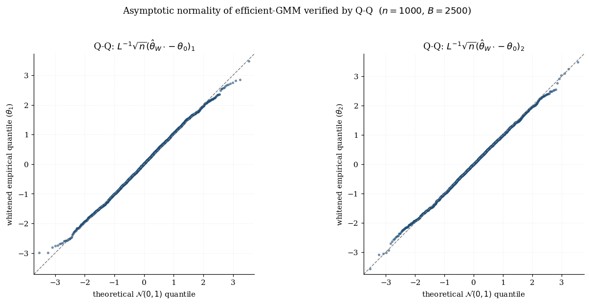
Step 4 — CLT on the moment vector at . by the classical CLT applied to i.i.d. with mean 0 and covariance .
Step 5 — Slutsky. . The limit is a linear transformation of a Gaussian: with and , so .
∎(Hansen 1982; textbook treatment in Newey & McFadden 1994 §2 and Hayashi 2000 Ch. 3.) The proof is structurally identical to the just-identified case of §2.3, with one substitution: instead of inverting directly (impossible in the over-identified case), we invert the first-order conditions . The mapping from ” moment-condition equations” to ” first-order-condition equations” is achieved by left-multiplying by , projecting the -dimensional moment residual onto the -dimensional parameter-direction subspace. This projection lives in the bread of the sandwich.
5.3 Reading the sandwich
The variance has three ingredients, each contributing a specific piece of statistical content. The Jacobian measures signal strength — how strongly the population moment responds to a parameter perturbation at the truth. A large (well-identified parameter, strong instruments) gives small . The covariance is the moment-noise covariance — diagonal entries capture per-moment noise levels, off-diagonals capture cross-moment correlations. The weighting matrix is the only ingredient under the analyst’s control: different ‘s produce different consistent estimators with different ‘s.
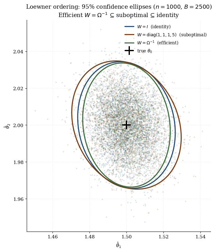
Three weighting values of practical interest: identity (, easy to compute, generally suboptimal); diagonal inverse-variance (, captures heteroskedasticity but ignores correlations); efficient (, achieves the Hansen bound). For score moments , the efficient sandwich collapses to , the Cramér–Rao bound — maximum likelihood is efficient GMM with score moments. The viz below makes the three ingredients literal: it shows how the bread / meat / sandwich operator-norms shift across weighting choices, and how the resulting 95% confidence ellipses nest.
In practice we don’t know or exactly. The natural plug-in estimators are
and the plug-in sandwich is . Under the regularity conditions of Theorem 5.1, , so confidence intervals built from have asymptotically correct coverage. For dependent data, is replaced by a HAC estimator like Newey–West.
5.4 Loewner ordering on asymptotic variances
Different choices of produce different asymptotic variances. We compare them via the Loewner ordering on positive-semidefinite matrices: . The Loewner ordering captures the variance comparison faithfully: means every linear combination of has smaller asymptotic variance under than under . Equivalently, every confidence ellipse from is contained in the corresponding ellipse from . The ordering is partial: not every two asymptotic-variance matrices are comparable. But there is a unique smallest element.
Question. Is there a that achieves for all positive-definite ?
Answer (proved in §6). Yes. The efficient weighting matrix uniquely (up to positive scaling) achieves the Loewner-minimum for every positive-definite .
§6 — Efficient weighting and the Hansen bound
§5 derived the sandwich asymptotic variance for any positive-definite and noted in §5.4 that the family has a Loewner-minimum. This section proves that the minimum is achieved uniquely (up to positive scaling) at , derives the resulting Hansen efficiency bound , and connects the bound to the semiparametric efficiency machinery from the prerequisite Semiparametric Inference. The agreement between Hansen’s purely algebraic argument and the Hilbert-space tangent-space construction of the semiparametric efficiency bound is one of the most satisfying results in this part of asymptotic statistics.
6.1 Minimizing the asymptotic variance
We want to find the positive-definite weighting matrix that minimizes in the Loewner order. Direct calculus on the matrix-valued objective is awkward — the cone of positive-definite matrices has no obvious differential structure that makes “differentiating with respect to ” tractable. The standard reduction is to scalar sub-problems: for every direction , find the that minimizes the scalar variance . If a single minimizes for every simultaneously, that is the Loewner-minimum of the family.
The strategy is global rather than local: we will not differentiate at all. Instead we exhibit directly and verify the Loewner inequality via a matrix Cauchy–Schwarz argument. This is Hansen’s original 1982 proof technique, and it generalizes the classical Gauss–Markov / Aitken theorem to nonlinear moment-condition models.
6.2 The efficient weighting matrix theorem
Theorem 6.1 (Efficiency of Ω⁻¹-weighted GMM).
Under the conditions of Theorem 5.1, for every positive-definite ,
with equality if and only if for some scalar .
Proof.
We invert and use matrix Cauchy–Schwarz, which is the cleaner form of the algebra.
Step 1 — whitening. Let be the Cholesky decomposition. Define and . Then is symmetric positive-definite, has full column rank , and
So and .
Step 2 — matrix Cauchy–Schwarz. For any matrices with invertible,
with equality iff . Proof: is the orthogonal projection onto , so is positive semi-definite, and .
Step 3 — apply with , . The pieces compute to . Inverting reverses the Loewner order:
Step 4 — uniqueness. Equality requires , which forces for some on . Translating back, .
∎(Hansen 1982; textbook treatment in Newey & McFadden 1994 §2.3.)
6.3 The Hansen efficiency bound
The single-matrix form — the Hansen efficiency bound — is structurally cleaner than the sandwich . The collapse from “bread × meat × bread” to a single matrix happens because under efficient weighting the meat equals the bread:
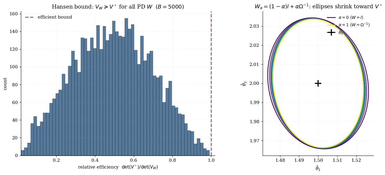
The visualization below makes this concrete. Panel A: a scatter of over 200 random positive-definite weighting matrices drawn from a Wishart distribution. sits at the southwest extreme — there is no that yields a smaller uncertainty volume and a smaller total uncertainty. Panel B: nested 95% confidence ellipses for the interpolation as slides from 0 (identity) to 1 (efficient).
6.4 Connection to the semiparametric efficiency bound
The Hansen bound admits a second derivation — entirely independent of Hansen’s algebra — from the semiparametric efficiency machinery developed in the prerequisite Semiparametric Inference. The two derivations are different proof technologies but they yield the same lower bound.
For the moment-condition model , the efficient influence function (EIF) for at is (Bickel–Klaassen–Ritov–Wellner 1993, Theorem 5.1)
Computing its variance:
The semiparametric bound equals the Hansen bound. Efficient GMM is therefore not merely efficient within the GMM family (Theorem 6.1) — it is efficient within the entire semiparametric class of RAL estimators of under the moment-condition restriction. No future ML, nonparametric, or regularized estimator can asymptotically beat on this model class. This is the rigorous statement of what makes GMM the canonical estimator for moment-condition models: it is information-theoretically optimal in the strongest sense available.
§7 — Two-step feasible efficient GMM
§6 proved that achieves the Hansen efficiency bound. But is a population object we do not observe. The two-step feasible efficient GMM procedure resolves this: run GMM once with some preliminary weighting to get a consistent first-step estimate , use those residuals to construct , then run GMM again with . The second-step estimator inherits the efficiency bound asymptotically. This is the practical algorithm of applied GMM; almost every GMM regression run in econometrics today follows this two-step structure.
7.1 The two-step algorithm
Algorithm 7.1 (Two-step efficient GMM (Hansen 1982)).
Given a sample and a moment function with :
- Choose a first-step weighting matrix , positive-definite and not depending on the parameter. Common choices: (always works), or for linear IV.
- First-step GMM: .
- Estimate from first-step residuals: .
- Second-step GMM with : .
- Return as the efficient estimator, with asymptotic variance .
Theorem 7.1 (Efficiency of the two-step estimator).
Under the conditions of Theorem 5.1, the two-step estimator from Algorithm 7.1 satisfies
Proof.
Two steps. Step 1: by consistency of (Theorem 4.1) combined with a uniform mean-value bound on over the neighborhood . Step 2: Apply Theorem 5.1 with (continuous mapping). The limit variance is .
∎The proof carries the central insight: the first-step weighting matrix doesn’t need to be efficient — it just needs to deliver consistency. Any positive-definite does the job. The efficiency comes entirely from the second-step weighting .
The visualization below traces Algorithm 7.1 end-to-end on the running example. Three stacked panels: (a) the step-1 criterion surface with the step-1 estimate marked; (b) the estimated shown as a heatmap (off-diagonals capture cross-sensor moment correlations); (c) the step-2 criterion surface , with step-1 and step-2 estimates overlaid. Raise to make the step-1 / step-2 ellipse shapes visibly different.
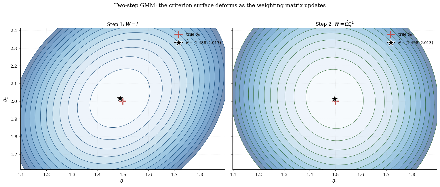
7.2 Estimating Ω from first-step residuals
For i.i.d. data the uncentered estimator (with ) is the natural choice — uncentered because by the moment-condition restriction. Some software packages center anyway (subtract ) as a defensive measure against misspecification; for correctly-specified models the two estimators are asymptotically equivalent.
For dependent data — time series, clustered samples — the simple covariance estimator is inconsistent because it ignores the contributions of at lags . The HAC estimator (Newey–West 1987; Andrews–Monahan 1991) generalizes:
where are sample auto-covariances, is a bandwidth, and is a kernel ensuring positive-definiteness. The canonical applied workflow: use Newey–West for time series, use the plain sample covariance for i.i.d. cross-sections.
7.3 Iterated GMM and convergence
The two-step procedure stops after one update of . Iterated GMM keeps going: re-estimate from residuals at , set , recompute , and iterate to a fixed point. Iterated GMM is a Picard iteration on the update map .
Three properties: (a) asymptotic equivalence — both and converge at rate with the same asymptotic variance ; (b) invariance — depends only on the sample and the moment function, not on ; (c) fixed-point characterization — for affine moment functions, this fixed point coincides with the continuous-updating estimator (CUE) of §10. In applied practice, two-step is the default; iterated GMM is used when reviewers ask for “specification-agnostic” results; CUE / EL / GEL (§10) are used when two-step bias matters.
7.4 Finite-sample bias of two-step GMM — the Hansen–Heaton–Yaron critique
Hansen, Heaton, and Yaron (1996) found that the estimated depends on the same data used in step 2, inducing a finite-sample bias of order . The mechanism: is constructed from , which is a function of the sample; using it as the weighting matrix in step 2 creates a correlation between and in the FOCs that classical asymptotics ignores.
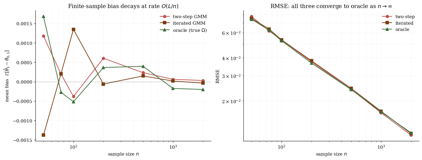
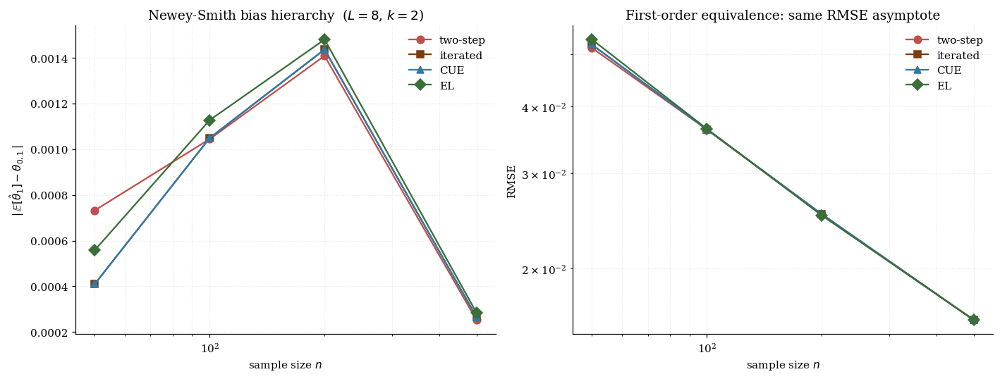
Three responses to the HHY critique shape the modern literature: iterated GMM mitigates but does not eliminate (bias drops by a constant factor); continuous-updating (CUE) jointly optimizes and with smaller higher-order bias; empirical likelihood (EL) has the smallest higher-order bias in the GEL class (Newey–Smith 2004). §10 develops all three.
§8 — The Hansen J-statistic and over-identification testing
The two-step procedure of §7 produces, almost as a by-product, a test of correct specification. The minimum value of the efficient-weight GMM criterion — the Hansen J-statistic — has an asymptotic distribution under correct specification. The same machinery that produces the point estimate produces a free specification test.
8.1 The J-statistic as a quadratic form
After running two-step (or iterated) efficient GMM, the Hansen J-statistic is
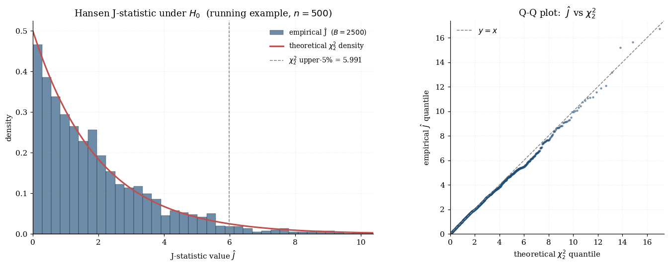
Under correct specification (), , so — bounded in probability, with the distribution below. Under misspecification (no satisfies the population moment condition), is bounded away from zero, so — the criterion diverges, and the test rejects with probability tending to 1.
8.2 Asymptotic distribution under H₀
Theorem 8.1 (Asymptotic distribution of the J-statistic).
Under the conditions of Theorem 5.1, with two-step or iterated efficient GMM weighting,
Proof.
Four steps.
Step 1 — linearize around . From the proof of Theorem 5.1, . Mean-value expansion of then gives
where is the residual-projection matrix.
Step 2 — CLT. . By continuous mapping and , .
Step 3 — whitening. Let and , . Then , where is the standard Euclidean orthogonal projection onto , a symmetric idempotent matrix of rank .
Step 4 — compute. . Since and is an orthogonal projection of rank , .
∎(Hansen 1982; the residual-projection proof is the canonical textbook treatment.) Geometric reading: the sample-moment vector at the GMM optimum is the residual after projecting the -dimensional moment-noise vector onto the -dimensional parameter-identifying subspace . The projection components are absorbed into ; the residual components are what measures. A just-identified model () has zero over-identifying restrictions, exactly, and there is no specification test. Over-identification is precisely the resource the J-test exploits.
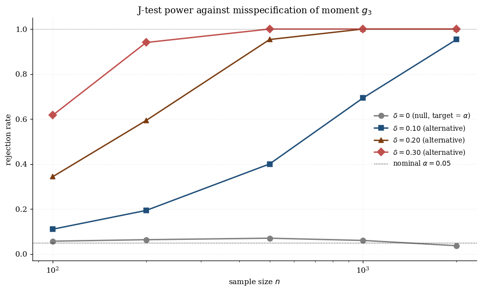
The visualization below runs the J-statistic Monte Carlo on the running example. Top panel: empirical density of over 400 two-step replicates at the user’s chosen , with the theoretical density overlaid. The empirical 95th percentile and Type-I rate are reported. Bottom panel: power curve — the empirical rejection rate at as we shift sensor 3’s true mean away from its -implied value by . At the rate hovers near ; as grows the rate rises toward 1, consistent with the consistency of the J-test against fixed misspecifications.
8.3 Power against misspecification
The J-test is consistent against any fixed misspecification: if the model is wrong, the test rejects with probability tending to 1.
Fixed alternatives. Suppose the true distribution satisfies for every . The “pseudo-true” parameter is the limit of , and the population objective at this point is strictly positive. So , at rate , and the test rejects with probability tending to 1.
Local alternatives (Pitman drift). Suppose the true population moment is for some fixed direction . Following the proof of Theorem 8.1 with the local-alternative drift, the limiting distribution is
— a non-central chi-squared. Power increases with : the J-test is most powerful against misspecifications that are large in the norm and orthogonal (in that norm) to the parameter-identifying subspace.
Where the J-test is blind. A misspecification — a deviation in the parameter-direction subspace — is absorbed by the GMM optimizer into a shift of and contributes nothing to . The J-test cannot detect parametric misspecification within the model’s identification capacity; it only detects mismatches orthogonal to the parameter-direction subspace.
8.4 Reading a J-test in practice
The standard reporting convention is the p-value: . Reject at level if . Three practical pitfalls.
Pitfall 1: “Low J → correctly specified” is a Type II error trap. A non-rejecting J-test is consistent with correct specification but does not prove it. Power against subtle misspecifications can be low at moderate .
Pitfall 2: A significant J does not localize the culprit. The J-statistic is a single scalar; it does not localize the problem to a specific moment condition. To diagnose, examine individual moment residuals ; the component(s) with the largest standardized residuals point to candidate misspecified moments. Newey (1985) develops formal tests of subsets of moment conditions.
Pitfall 3: Weak identification inflates the false-rejection rate. When is near-singular, the asymptotic approximation breaks down. The Anderson–Rubin test (§9.4) provides a weak-instrument-robust alternative.
Relationship to other specification tests. The Sargan test (Sargan 1958) is the J-test specialized to linear IV — same statistic, same null distribution, older econometric name. The Hausman test (Hausman 1978) tests whether two consistent estimators agree — a specification check based on the difference between estimators. Conditional moment tests (Newey 1985) test subsets of moment conditions, useful for localizing the source of a significant J-statistic.
§9 — Linear GMM, instrumental variables, and 2SLS
This section makes the abstract framework concrete via the canonical applied case: linear instrumental-variables regression. The IV setting is where GMM was born — Hansen and Singleton’s (1982) Euler equations are nonlinear IV — and where the framework continues to do most of its applied work.
9.1 The linear IV model
The structural equation is , , where is a vector of regressors with some component endogenous, . OLS is biased because the orthogonality condition fails.
The fix is an instrument vector with satisfying two conditions: exogeneity and relevance has rank . Given , the GMM moment function is . By exogeneity, at the truth. By relevance, has full column rank . The over-identification degree is .
The sample-moment vector is where stack rows. The sample Jacobian is , independent of (the moment function is affine in ).
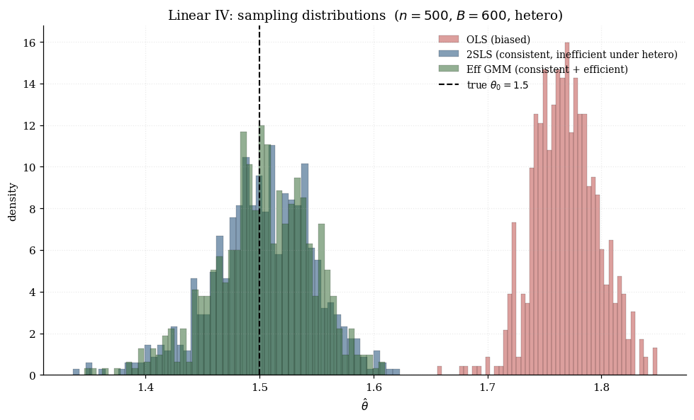
The visualization below sets (one endogenous regressor) and (four instruments), with a heteroskedasticity-controlled error variance. As you raise endogeneity , the OLS sampling distribution drifts away from . As you raise heteroskedasticity , the efficient-GMM advantage over 2SLS grows.
9.2 2SLS as -weighted GMM
The GMM estimator with a generic weighting matrix is
closed-form because is affine in .
Theorem 9.1 (2SLS as GMM).
The two-stage least squares estimator is the GMM estimator with weighting matrix :
Proof.
Substitute into (9.1); the scalar cancels, leaving .
∎The textbook “two-stage” interpretation: is the OLS prediction of from (first stage), and is the OLS regression of on (second stage). Under homoskedasticity , , and differs from only by the scalar . So 2SLS is efficient GMM under homoskedasticity. The Hansen bound becomes , estimated as — the standard 2SLS variance formula.
9.3 Efficient GMM under heteroskedasticity
When depends on , is no longer proportional to , and 2SLS is inefficient. The fix is the two-step procedure of §7 specialized to linear IV.
Algorithm 9.1 (Heteroskedasticity-robust efficient GMM).
- Run 2SLS to obtain .
- Compute residuals .
- Estimate the heteroskedasticity-robust moment covariance: .
- Re-estimate GMM with : .
- The plug-in efficient variance is .
This estimator goes by several names: efficient GMM (Hansen 1982), heteroskedasticity-robust 2SLS (applied econometrics), White (1980) estimator in the just-identified case , or sandwich estimator (statistical learning).
9.4 Weak instruments and near-identification
For a scalar endogenous regressor (), the first-stage equation is . The strength of the instruments is measured by the concentration parameter . The first-stage F-statistic is (large- approximation), an asymptotic chi-squared random variable under the null that all .
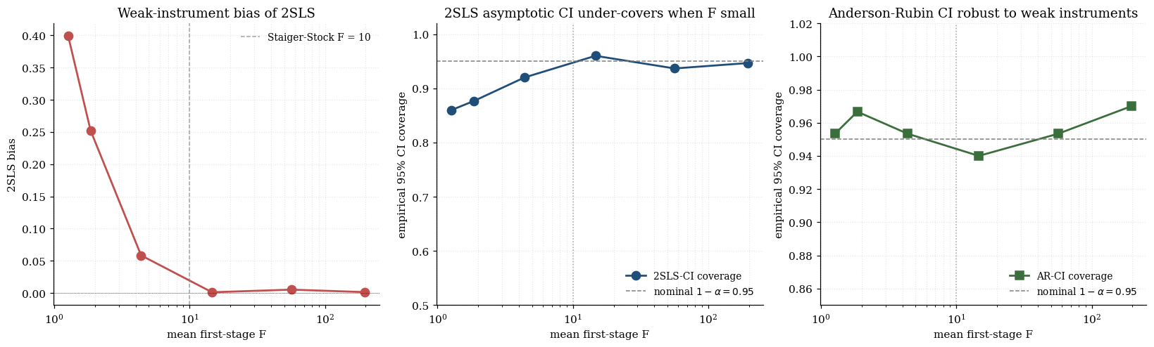
Staiger and Stock (1997, Econometrica 65(3): 557–586) proposed the most-cited rule of thumb — first-stage F > 10 as a working threshold separating “strong” from “weak” identification — based on simulation evidence that the 2SLS asymptotic-normal approximation deteriorates below this point. Stock and Yogo (2005) subsequently formalized the threshold via tabulated critical values: under their bias-bound criterion (2SLS bias of OLS bias) at instrument, the 5%-level critical value is approximately 11.0; values for other pairs are in Stock-Yogo Tables 1–2.
When the first-stage F is below 10, two pathologies appear. Bias: 2SLS becomes biased toward OLS in finite samples, with bias of order . Standard-error distortion: the 2SLS asymptotic-normal CI undercovers — the nominal-95% CI may have actual coverage of 80% or less.
The Anderson–Rubin test (Anderson and Rubin 1949) introduced a test that does not condition on estimating and is therefore robust to weak instruments. The AR statistic at a hypothesized value is
where is the moment-covariance estimated under . Under , by the same residual-projection argument as §8.2 but without subtracting the parameter-estimation degrees of freedom,
The AR confidence set is — robust to weak instruments. Kleibergen (2002) developed the K-statistic and Moreira (2003) the conditional-likelihood-ratio test as closely related weak-instrument-robust alternatives.
The visualization below makes the weak-instrument failure mode visible. Slide the first-stage strength down toward zero: the 2SLS sampling distribution develops bias toward OLS and heavy tails, while the AR confidence set widens dramatically (often spanning the whole real line) to honestly reflect the lost identification. The 2SLS Wald 95% CI under-covers — its width does not grow as shrinks.
For ML / causal-inference applications with strong, theory-motivated instruments (e.g., randomized experiments treated as instruments for compliance), weak instruments are rarely binding. For applied micro applications relying on borderline-relevant instruments, the weak-instrument diagnostics are essential.
§10 — Modern GMM: CUE, empirical likelihood, and GEL
Three modern estimators — the continuous-updating estimator (CUE), Owen’s empirical likelihood (EL), and the generalized empirical likelihood (GEL) family unifying both — provide alternatives to two-step GMM with the same first-order asymptotic efficiency but provably smaller higher-order bias. Newey and Smith (2004) gave the unifying analysis: CUE, EL, and exponential tilting (ET) are all members of a single one-parameter family with a bias hierarchy where EL is strictly preferred.
10.1 The continuous-updating estimator (CUE)
CUE collapses the two steps into a single joint optimization:
where is recomputed at every . The criterion is genuinely nonlinear, even when is affine in .
Three properties of CUE: (a) smaller higher-order bias than two-step GMM — CUE breaks the – asymmetry; (b) reparametrization invariance — invariant to smooth invertible ; (c) computational cost — nonlinear optimization (BFGS or Newton) starting from the two-step estimate; typically iterations. Under standard regularity with the same as two-step.
10.2 Empirical likelihood (Owen 1988, 1990, 2001)
Empirical likelihood replaces the parametric likelihood with a nonparametric likelihood defined over discrete distributions supported on the data. Given probability weights , define the empirical likelihood subject to , , and .
Profile empirical likelihood. At each , profile out . The Lagrangian KKT conditions give , where solves the inner moment constraint
The inner problem (10.1) is the FOC of a convex optimization over — minimize — with unique interior solution. Newton-Raphson with backtracking (to maintain ) converges in iterations.
The profile empirical-likelihood-ratio statistic is , and the empirical likelihood estimator is .
Theorem 10.1 (Wilks' theorem for empirical likelihood (Owen 1990)).
Under the conditions of Theorem 5.1, — the parametric Wilks asymptotic, despite the nonparametric construction. The EL over-identification statistic satisfies — the same degrees of freedom as Hansen’s J-statistic.
EL confidence regions are transformation-invariant, have data-determined shape, and have better finite-sample coverage in many settings (DiCiccio-Hall-Romano 1991).
10.3 Generalized empirical likelihood (GEL): the Newey–Smith unification
Newey-Smith (2004) observed that CUE, EL, and ET all fit a single GEL family. Let be twice continuously differentiable, concave on a neighborhood of zero, with . The GEL estimator with carrier is
Three canonical members of the Cressie-Read family :
| Estimator | Source | ||
|---|---|---|---|
| CUE | Hansen-Heaton-Yaron 1996 | ||
| EL | Owen 1988, 1990 | ||
| (centered) | ET | Imbens 1997; Kitamura-Stutzer 1997 |
All GEL estimators have — first-order equivalent.
10.4 Higher-order properties and the Newey–Smith bias hierarchy
Newey-Smith (2004) computed the bias for each estimator and proved a strict ordering:
The visualization below makes the hierarchy visible. Panel A: the Cressie-Read carrier morphs as you slide — at it’s the EL log carrier; at the CUE quadratic; at the ET exponential. Panel B: an empirical bar chart of mean for two-step, iterated, CUE, and EL on the running example at small where the gap is visible.
Computational hierarchy:
| Estimator | Implementation | Per-replicate cost |
|---|---|---|
| Two-step GMM | Closed-form (linear) / 2 BFGS (nonlinear) | |
| Iterated GMM | Picard iteration | |
| CUE | Single BFGS with -dependent | |
| EL | Nested BFGS + Newton on | |
| ET | Same as EL with exponential carrier | similar to EL |
Recommendation. Modern applied workflow: (1) always report two-step efficient GMM as the baseline; (2) also report CUE or EL when is large or ; (3) use EL-based confidence regions when interest centers on a nonlinear function of .
§11 — GMM and maximum likelihood
Maximum likelihood is the canonical estimator of parametric statistics. GMM is the canonical estimator of moment-condition models. ML is just-identified GMM with the score equations as moment conditions, and the Cramér–Rao bound is the Hansen efficiency bound under score moments. Conversely, when the assumed likelihood is wrong, the resulting “quasi-MLE” is consistent for a pseudo-true parameter but inherits the GMM sandwich variance rather than the Fisher-information inverse. Every M-estimator — MLE, OLS, quantile regression, Huber regression, quasi-MLE — is just-identified GMM with a specific score-like moment function. GMM extends M-estimation by allowing .
11.1 ML as just-identified GMM
The MLE solves . Identify the score with the moment function: . The MLE is the just-identified GMM estimator with . Under regularity:
- (the score has mean zero at the truth).
- (Hessian of the log-likelihood in expectation = negative Fisher information).
- (the information matrix equality; Fisher 1925).
Substituting into the just-identified sandwich:
The MLE achieves the Cramér–Rao lower bound. From the §6 perspective: . So MLE is efficient GMM with score moments — and the Cramér–Rao bound is the moment-condition special case of the Hansen efficiency bound.
11.2 Quasi-MLE and the sandwich variance
What if we maximize a wrong likelihood? Suppose the data come from but we maximize for a working density . The estimator solves and is called the quasi-MLE.
The quasi-MLE is consistent for the pseudo-true parameter . Under misspecification, the information matrix equality fails: . The quasi-MLE asymptotic variance is the GMM sandwich:
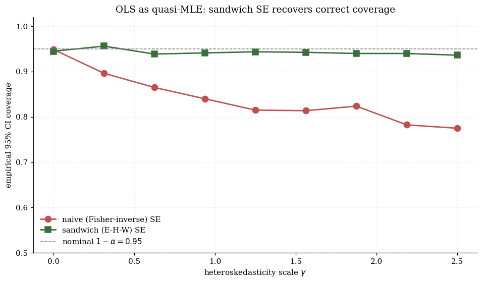
This is the Eicker–Huber–White sandwich (Eicker 1967; Huber 1967; White 1980), familiar as “robust standard errors” or vcov_type='HC0'.
Canonical example: heteroskedastic OLS. under the working assumption of homoskedastic Gaussian errors. OLS is the quasi-MLE. Under homoskedasticity, the information matrix equality holds and the naive CI has correct coverage. Under heteroskedasticity, the equality fails and the naive CI under-covers; the sandwich CI restores nominal coverage. The visualization below makes this concrete: slide the heteroskedasticity scale up and watch the naive coverage drop while the sandwich stays near 95%.
11.3 M-estimation as a unifying framework
Pick a loss function and define . The FOC with is just-identified GMM with . The asymptotic variance is the sandwich .
Five M-estimators:
| Estimator | Information identity holds? | ||
|---|---|---|---|
| MLE | Yes (correctly specified) | ||
| Quasi-MLE | No (misspecified) | ||
| OLS | Only under homoskedastic Gaussian | ||
| Quantile regression () | No (non-smooth) | ||
| Huber regression | No |
where (Koenker-Bassett 1978) and is the Huber loss (Huber 1964). Where GMM extends M-estimation. The over-identified case has no counterpart in classical M-estimation: there is no whose gradient is the full -vector . GMM absorbs M-estimation when and strictly generalizes it when by introducing the weighting matrix . In modern causal inference (§12), this generalization is the substantive value of GMM.
§12 — GMM in modern causal inference
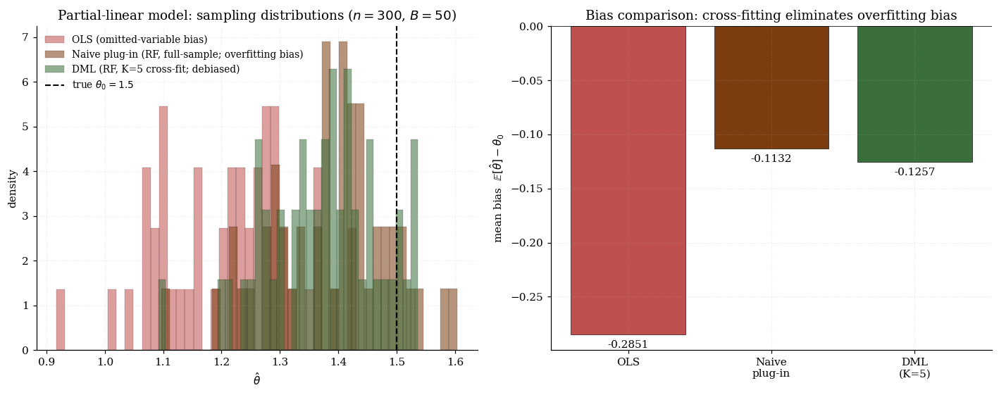
The most active recent application of GMM is in causal inference with machine-learned nuisance functions — what Chernozhukov, Chetverikov, Demirer, Duflo, Hansen, Newey, and Robins (2018) call double / debiased machine learning (DML). We want to estimate a low-dimensional causal parameter but identification requires high-dimensional nuisance functions estimated with ML at sub-parametric rates. DML answers: how can we plug ML-estimated into a target-parameter estimator and still get -consistent, asymptotically-normal ?
The answer combines two ideas: Neyman orthogonality — design so that — and cross-fitting — estimate on one fold, evaluate on another fold. Under both, achieves -consistency and asymptotic normality even when converges at rate, and the asymptotic variance is the semiparametric efficiency bound.
12.1 Doubly robust estimation as GMM
The partial-linear model. Observe where
Nuisances where . The Robinson (1988) partialling-out construction: given , form residuals , . The estimator is the simple OLS slope . This is GMM with the Robinson moment .
For the average treatment effect with binary treatment , the AIPW moment is
with . The estimator has the double robustness property: consistent if either the outcome regressions are consistent or the propensity is consistent.
12.2 Double machine learning
Algorithm 12.1 (DML, K-fold cross-fitting).
- Partition the data into folds .
- For each : estimate on observations outside fold ; evaluate on observations in fold .
- Solve the cross-fitted moment equation for .
Theorem 12.1 (Chernozhukov et al. (2018)).
Assume the moment function is Neyman-orthogonal (§12.3) and the product of nuisance estimation errors satisfies — the mixed-bias condition (a standard sufficient condition is for each nuisance). Under standard regularity (smooth , bounded moments, identification at ),
where is the semiparametric efficiency bound.
The result is striking. With ML nuisance estimators converging at rather than the parametric , the DML point estimator still attains -rate and Gaussian asymptotic inference, and achieves the semiparametric efficiency bound. The “double” in DML refers to the mixed-bias product condition: the product of the two nuisance error rates only needs to be — a substantially weaker requirement than the -each rate the naive plug-in argument would demand.
The visualization below illustrates the bias hierarchy on a partial-linear DGP with nonlinear nuisances , , fit with degree-4 polynomial regression (a simpler-than-RF nuisance estimator that still exhibits the asymptotic story). The bar chart shows bias and SD across replicates for the three estimators; the histogram shows the sampling distributions overlaid. OLS is biased because it doesn’t adjust for ; naive plug-in is biased at moderate because the same data fits nuisances and structural estimator; DML cross-fits and the bias collapses.
12.3 Neyman orthogonality: the central design constraint
The DML construction works because satisfies Neyman orthogonality:
This is a pathwise / Gâteaux derivative condition: small perturbations of around leave the population expectation of unchanged to first order. The plug-in estimator is therefore first-order insensitive to .
Verifying orthogonality for the Robinson moment. With , perturbing gives , with using . Similarly , with . The Robinson moment is Neyman orthogonal by construction.
Constructing orthogonal moments via the EIF. Start with a “naive” moment satisfying but not Neyman orthogonal. The orthogonalized moment is , where is the EIF of the nuisance-correction term from the semiparametric efficiency machinery (§6.4). This Neyman orthogonalization is the same operation that produces AIPW from naive outcome regression, Robinson partialling-out from naive OLS, targeted minimum-loss from naive plug-in, and most modern doubly-robust estimators.
Three reasons GMM-with-ML-nuisances is the modern frontier: (1) asymptotic theory is portable — Theorem 5.1’s sandwich, §6’s efficiency bound, §8’s J-statistic all generalize; (2) multiple identifying moments combine optimally — efficient GMM with the union of moments achieves the semiparametric efficiency bound; (3) specification testing is free — Hansen’s J-statistic generalizes to the DML setting (Chernozhukov-Newey-Singh 2022).
§13 — Computational notes, limits, and connections
13.1 Numerical optimization tips
Affine moment functions: use the closed form. numpy.linalg.solve(A.T @ W @ A, A.T @ W @ b) computes the GMM estimate in microseconds. Do not call scipy.optimize.minimize on a linear problem. For smooth nonlinear moments, scipy.optimize.minimize(method='BFGS') with the two-step estimate as starting value is the practical default; pass analytic gradients via jac= when available.
The CUE objective is generally nonconvex even for affine moments. Starting from the two-step estimate — asymptotically equivalent to CUE — typically lands in the convex basin of the global minimum. For EL, use nested optimization with a convex inner problem: Newton-Raphson with line search on the inner (converges in iterations), BFGS on the profile as the outer loop.
Convergence diagnostics: monitor the norm of the FOC residual at the optimum (should be near machine epsilon), the condition number of (large = weak identification), and the J-statistic value vs critical (large = specification rejection). Multi-start optimization is the standard defensive strategy for nonconvex problems.
13.2 Bootstrap for GMM and the J-statistic
The naïve nonparametric bootstrap fails for GMM because the bootstrap moment condition is not zero at in the over-identified case. The Brown-Newey (1995) / Hall-Horowitz (1996) recentered bootstrap fixes this: define and run GMM on . Hall and Horowitz (1996) proved that the recentered bootstrap yields an asymptotic refinement: bootstrap CIs and J-test critical values have coverage error vs asymptotic. Modern variants: wild bootstrap (Davidson-MacKinnon 2010) for heteroskedasticity-robust refinement; block bootstrap (Künsch 1989) for time-series GMM. Default for most applied work: recentered bootstrap with .
13.3 Bayesian GMM via Chernozhukov–Hong (2003)
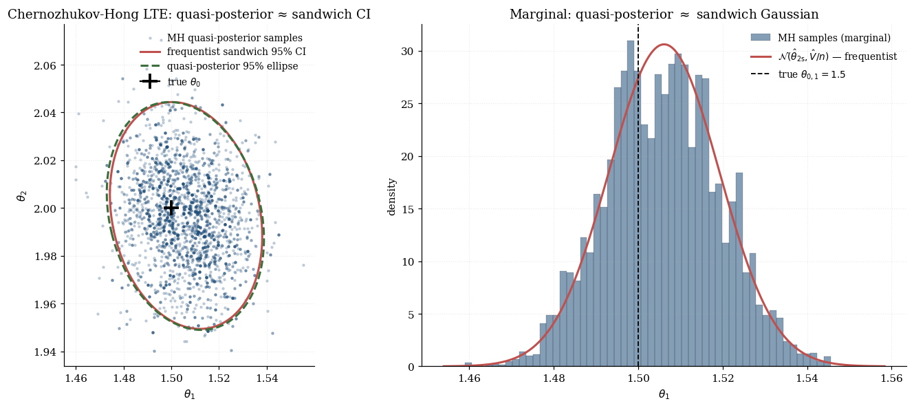
Chernozhukov-Hong define a Laplace-type estimator (LTE) by treating the GMM criterion as a quasi-log-likelihood:
Under standard regularity, the posterior mean is consistent, posterior variance equals the GMM sandwich variance, and posterior credible regions equal asymptotic confidence regions to first order. The visualization below runs a 2D random-walk Metropolis sampler from this quasi-posterior on the running example. Top panel: the LTE sample cloud overlaid with the frequentist sandwich 95% ellipse — the two agree at moderate . Bottom panel: marginal posterior densities for and , with the Gaussian asymptotic curves overlaid.
LTE is useful when: the GMM criterion is non-smooth (quantile IV, M-estimation with non-differentiable loss); the criterion is multimodal; the model is weakly identified and MCMC reveals the indeterminate direction; informative prior information is available.
13.4 Cross-site connections and further reading
Inbound connections from sister sites. The just-identified predecessor is formalStatistics: method-of-moments , which develops the §2 Pearson construction in detail. The deferred reciprocal in docs/plans/deferred-reciprocals.md auto-discharges via the formalstatisticsPrereqs reciprocal on ship.
Outbound connections within formalML. Three previously-shipped topics underwrite GMM’s machinery: Concentration Inequalities (uniform-LLN bridge for the §4 consistency proof), Convex Analysis (convex-quadratic geometry of the GMM criterion), and Semiparametric Inference (efficient influence function and the semiparametric efficiency bound that equals the Hansen bound). Two planned formalML topics will pick up where GMM leaves off: Causal Inference Methods (coming soon) — doubly-robust estimation, double machine learning, Neyman orthogonality, AIPW; and Empirical Processes (coming soon) — formal development of uniform LLN and Glivenko-Cantelli machinery.
Recommended further reading. Original sources: Hansen (1982), Hansen-Singleton (1982), Owen (1988). Textbook treatments: Hayashi (2000) Ch. 3-5; Hansen B.E. (2022) Ch. 13-15 (free online); Newey-McFadden (1994). Modern developments: Newey-Smith (2004) for GEL unification; Chernozhukov et al. (2018) for DML; Kennedy (2022) for EIF formulas. Software: linearmodels (Python); gmm package (R); statsmodels.sandbox.regression.gmm (Python); ivreg2 (Stata). For DML: econml (Microsoft); doubleml (CRAN/PyPI).
Closing remark. GMM is one of the few estimation frameworks that has stayed central through forty years of changing computational tools. Pearson’s method of moments (1894) became Hansen’s GMM (1982) became Newey-Smith’s GEL (2004) became Chernozhukov et al.’s DML (2018). Each generation built on the same algebraic core — minimize a weighted quadratic in the sample-moment vector — and adapted it to the computational reality of the day. The modern incarnation, GMM with cross-fitted ML nuisances, is the framework that lets us put random forests inside causal-inference confidence intervals without giving up the -consistency that classical statistics requires.
Connections
- The uniform LLN required for the §4 consistency proof comes directly from the empirical-process / Talagrand machinery developed there. Pointwise convergence of the sample-moment vector at each θ is not enough — the GMM estimator is an argmin, and we need sup_θ ‖ḡ_n − m‖ →_p 0 to conclude argmin convergence. The bracketing-entropy and Rademacher-complexity routes both deliver this. concentration-inequalities
- The GMM criterion J_n(θ, W) = n ḡ_n(θ)ᵀ W ḡ_n(θ) is a convex quadratic form in the sample-moment residual. When g(X, θ) is affine in θ (the linear IV / running-example case), J_n is globally convex in θ with a closed-form minimizer; for nonlinear g it is convex on a neighborhood of θ₀. The first-order conditions of §3.3 are the convex normal equations. convex-analysis
- The Hansen efficiency bound V* = (G₀ᵀ Ω⁻¹ G₀)⁻¹ equals the semiparametric efficiency bound for the moment-condition model — derivable independently via the efficient influence function (§6.4). The DML machinery of §12 is exactly Neyman-orthogonalized GMM with ML-estimated nuisance functions; the orthogonalization step uses the same EIF construction. semiparametric-inference
References & Further Reading
- paper Contributions to the Mathematical Theory of Evolution — Pearson (1894) Philosophical Transactions of the Royal Society A 185: 71–110. The introduction of the method of moments.
- paper Large Sample Properties of Generalized Method of Moments Estimators — Hansen (1982) Econometrica 50(4): 1029–1054. The foundational GMM paper.
- paper Generalized Instrumental Variables Estimation of Nonlinear Rational Expectations Models — Hansen & Singleton (1982) Econometrica 50(5): 1269–1286. The asset-pricing application that motivated GMM.
- paper Estimation of the Parameters of a Single Equation in a Complete System of Stochastic Equations — Anderson & Rubin (1949) Annals of Mathematical Statistics 20(1): 46–63. The AR weak-instrument-robust test.
- paper Theory of Statistical Estimation — Fisher (1925) Proceedings of the Cambridge Philosophical Society 22(5): 700–725. The information matrix equality.
- paper Empirical Likelihood Ratio Confidence Intervals for a Single Functional — Owen (1988) Biometrika 75(2): 237–249. The introduction of empirical likelihood.
- paper Empirical Likelihood Ratio Confidence Regions — Owen (1990) Annals of Statistics 18(1): 90–120. Wilks' theorem for empirical likelihood.
- paper The Estimation of Economic Relationships Using Instrumental Variables — Sargan (1958) Econometrica 26(3): 393–415. The Sargan test (special case of Hansen's J).
- paper A Heteroskedasticity-Consistent Covariance Matrix Estimator and a Direct Test for Heteroskedasticity — White (1980) Econometrica 48(4): 817–838. The Eicker–Huber–White sandwich estimator.
- paper Finite Sample Properties of Some Alternative GMM Estimators — Hansen, Heaton & Yaron (1996) Journal of Business and Economic Statistics 14(3): 262–280. Introduces the CUE and quantifies two-step bias.
- paper An MCMC Approach to Classical Estimation — Chernozhukov & Hong (2003) Journal of Econometrics 115(2): 293–346. The Laplace-type estimator.
- paper Multinomial Goodness-of-Fit Tests — Cressie & Read (1984) Journal of the Royal Statistical Society B 46(3): 440–464. The Cressie–Read divergence family.
- paper Bootstrap Critical Values for Tests Based on Generalized-Method-of-Moments Estimators — Hall & Horowitz (1996) Econometrica 64(4): 891–916. Recentered bootstrap for GMM.
- paper Specification Tests in Econometrics — Hausman (1978) Econometrica 46(6): 1251–1271.
- paper One-Step Estimators for Over-Identified Generalized Method of Moments Models — Imbens (1997) Review of Economic Studies 64(3): 359–383. Information-theoretic alternatives to GMM.
- paper An Information-Theoretic Alternative to Generalized Method of Moments Estimation — Kitamura & Stutzer (1997) Econometrica 65(4): 861–874. Exponential tilting estimator.
- paper Pivotal Statistics for Testing Structural Parameters in Instrumental Variables Regression — Kleibergen (2002) Econometrica 70(5): 1781–1803. The K-statistic for weak instruments.
- paper A Conditional Likelihood Ratio Test for Structural Models — Moreira (2003) Econometrica 71(4): 1027–1048. Conditional LR for weak-instrument-robust inference.
- paper Generalized Method of Moments Specification Testing — Newey (1985) Journal of Econometrics 29(3): 229–256. Conditional moment tests.
- paper Large Sample Estimation and Hypothesis Testing — Newey & McFadden (1994) Handbook of Econometrics Vol. 4, Ch. 36. The textbook treatment of GMM asymptotics.
- paper Higher Order Properties of GMM and Generalized Empirical Likelihood Estimators — Newey & Smith (2004) Econometrica 72(1): 219–255. Unifies CUE, EL, and ET in the GEL family.
- paper Root-N-Consistent Semiparametric Regression — Robinson (1988) Econometrica 56(4): 931–954. The partial-linear estimator.
- paper Instrumental Variables Regression with Weak Instruments — Staiger & Stock (1997) Econometrica 65(3): 557–586. First-stage F > 10 rule of thumb.
- book Testing for Weak Instruments in Linear IV Regression — Stock & Yogo (2005) Identification and Inference for Econometric Models, ed. Andrews & Stock, 80–108.
- paper Double/Debiased Machine Learning for Treatment and Structural Parameters — Chernozhukov, Chetverikov, Demirer, Duflo, Hansen, Newey & Robins (2018) Econometrics Journal 21(1): C1–C68. The DML framework.
- book Econometrics — Hayashi (2000) Princeton University Press. Chapters 3–5 cover GMM in textbook form.
- book Empirical Likelihood — Owen (2001) Chapman & Hall/CRC Monographs on Statistics and Applied Probability 92.