Adjunctions
The free-forgetful paradigm, unit-counit pairs, and the universal optimization pattern that connects algebra, logic, and machine learning
Overview & Motivation
Consider a problem we’ve already encountered concretely. You have a set and a vector space . You want to define a linear map from “the vector space built from ” to . The free vector space has basis , so . A linear map is determined by the matrix — that is, by specifying where the two basis elements go. But specifying where basis elements go is just a function . We’ve established a bijection:
where is the underlying set of (forgetting the vector space structure). This bijection is not a coincidence — it’s a natural isomorphism, and the pattern it instantiates is called an adjunction.
An adjunction between categories and says: for every and , there is a bijection
that is natural in both variables. The left adjoint “freely builds structure,” and the right adjoint “forgets structure.” This free-forgetful pattern appears everywhere:
- Free groups: — a group homomorphism from is determined by where generators go.
- Products: — a morphism into a product is a pair of morphisms.
- Tensor-hom: — bilinear maps from to correspond to linear maps . This is currying.
- Quantifiers: — the existential and universal quantifiers are adjoints of substitution in logical syntax.
For machine learning, adjunctions formalize Lagrangian duality as a Galois connection between primal and dual optimization problems, the encoder-decoder paradigm as a pair of approximately inverse functors, and attention mechanisms as instances of the tensor-hom adjunction (currying).
Every adjunction also generates a monad — the round-trip composition that “freely builds and then forgets.” This connects adjunctions to the capstone of the Category Theory track.
Roadmap. We develop three equivalent definitions (Hom-set, unit-counit, universal morphism), prove their equivalence, then turn to properties: uniqueness of adjoints (via Yoneda), composition, and the RAPL theorem. Galois connections specialize adjunctions to posets, giving concrete examples from number theory, topology, and optimization. We close with the Adjoint Functor Theorem, ML connections, and a preview of monads.
Adjunctions: The Hom-Set Definition
We begin with the most symmetric formulation.
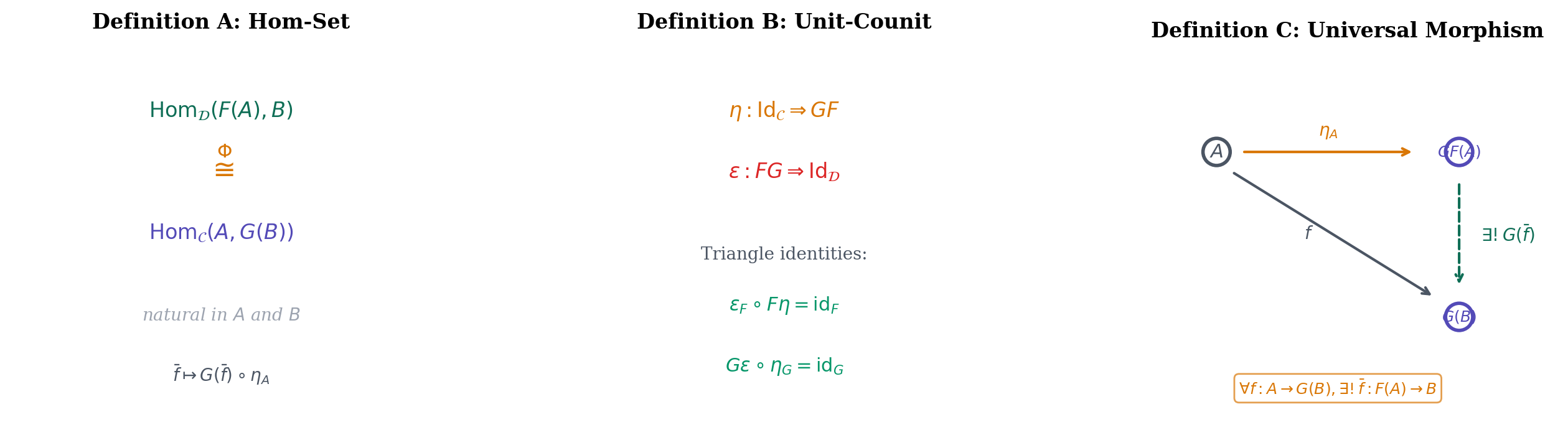
Definition 1 (Adjunction (Hom-Set)).
Let and be categories, and let and be functors. An adjunction (read ” is left adjoint to ”) is a natural isomorphism
for all , , natural in both and .
We call the left adjoint and the right adjoint.
Naturality in both variables means: for any morphism in and in , the following diagrams commute:
The bijection gives every morphism in a unique partner in .
Definition 2 (Adjoint Transpose).
Given an adjunction with natural isomorphism , the adjoint transpose of a morphism is
Conversely, the adjoint transpose of is .
Example. In the free-forgetful adjunction , if and , then a function with and has adjoint transpose given by the matrix
The columns are exactly and — the images of the basis elements. This is the free-forgetful bijection at work.
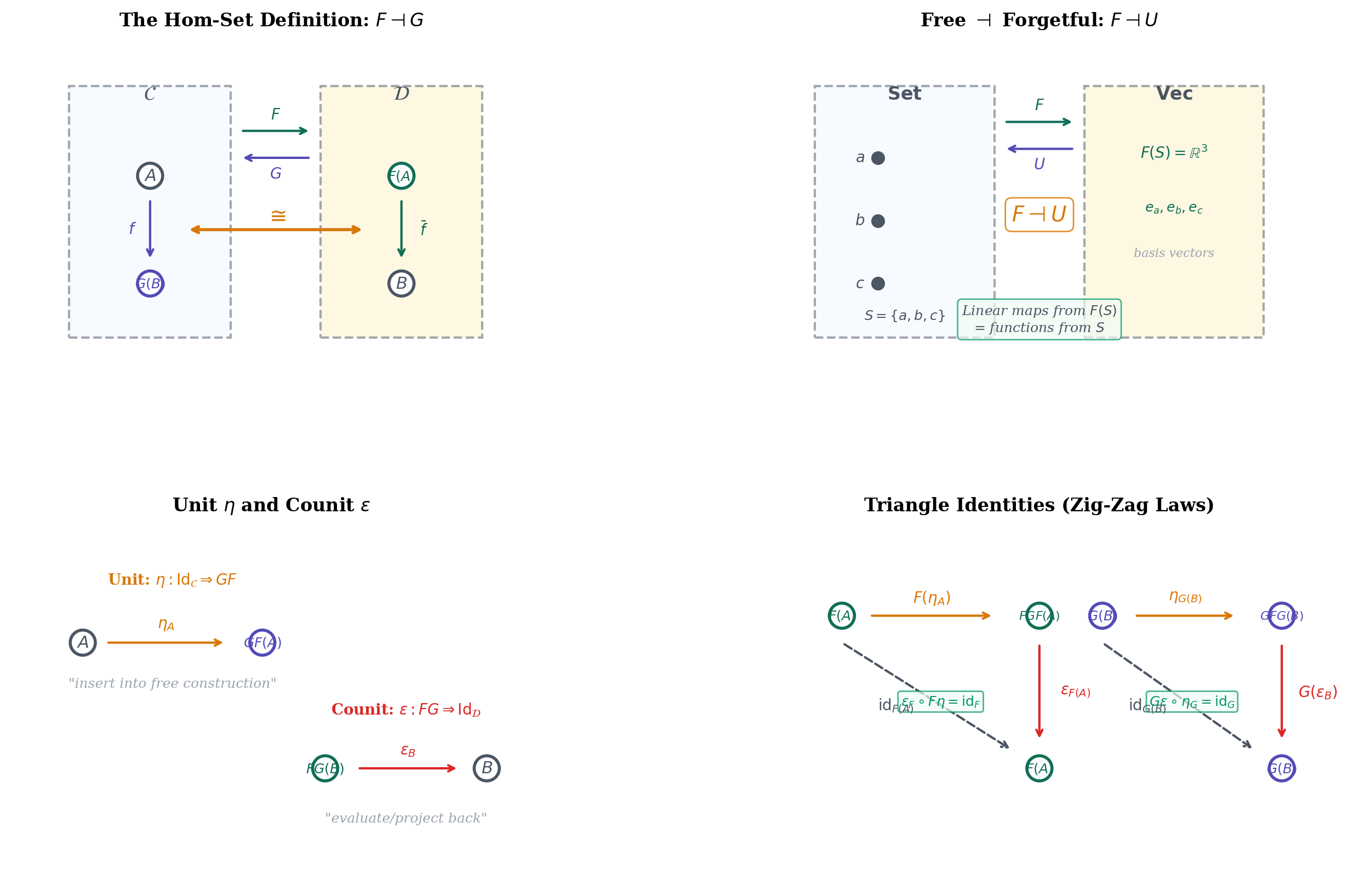
Free ⊣ Forgetful (Set ↔ Vec): a linear map from F(S) is determined by where basis elements go — just a function from S.
εF ∘ Fη = idF : ✓
Gε ∘ ηG = idG : ✓
Unit, Counit, and the Triangle Identities
The Hom-set definition is elegant, but it hides the concrete data that makes an adjunction tick. The unit-counit formulation exposes that data.
Definition 3 (Unit of an Adjunction).
Given an adjunction with isomorphism , the unit is the natural transformation defined by
for each . The unit “inserts into the round-trip .”
Definition 4 (Counit of an Adjunction).
The counit is the natural transformation defined by
for each . The counit “evaluates the round-trip back to .”
Example. In the free-forgetful adjunction, the unit is the basis insertion: . It takes each element of and maps it to the corresponding basis vector in the free vector space. The counit is the evaluation map: the free vector space on the underlying set of maps back to by extending the identity linearly.
The unit and counit are connected by a remarkable pair of equations.
Definition 5 (Triangle Identities (Zig-Zag Laws)).
The triangle identities for an adjunction with unit and counit are:
In string diagram notation, these are the “zig-zag” equations — each composition snakes up and back, then collapses to the straight line (the identity).
The first says: if we start at , go up via to , then come back down via to , we end up where we started. The second is the dual statement for .
Definition 6 (Adjunction (Unit-Counit)).
An adjunction consists of functors , and natural transformations (the unit) and (the counit) satisfying the triangle identities.
A Gallery of Adjunctions
Adjunctions appear throughout mathematics once we know what to look for. The pattern is always the same: a “free” construction that builds structure from raw material, paired with a “forgetful” functor that strips structure away.
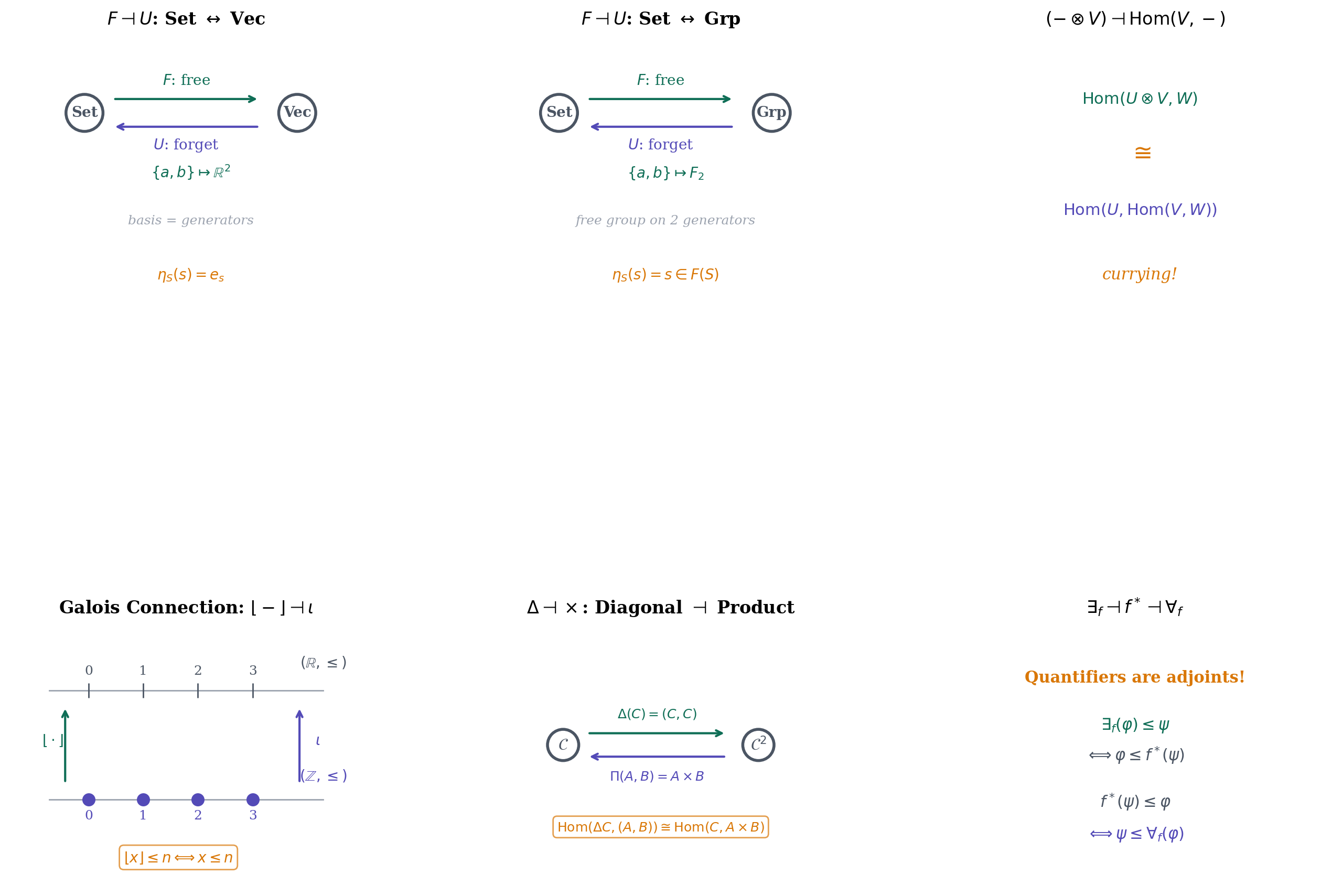
1. Free ⊣ Forgetful (Set ↔ Vec). free vector space on , underlying set of . A linear map from is determined by where the basis goes. This is our running example.
2. Free ⊣ Forgetful (Set ↔ Grp). free group on , underlying set of . A group homomorphism from is determined by where generators go. For , we get , and every group homomorphism is determined by the image of — an arbitrary element of .
3. Diagonal ⊣ Product. sends to . Its right adjoint sends to the product . The adjunction says:
A morphism into a product is determined by a pair of morphisms — this is the universal property of products, repackaged as an adjunction.
4. Coproduct ⊣ Diagonal. Dually, sends to , with as right adjoint:
A morphism out of a coproduct is a pair of morphisms.
5. Tensor-Hom (Currying). In , :
A bilinear map from corresponds to a linear map from to the space of linear maps . This is the categorification of currying from functional programming — and it underlies the attention mechanism in transformers.
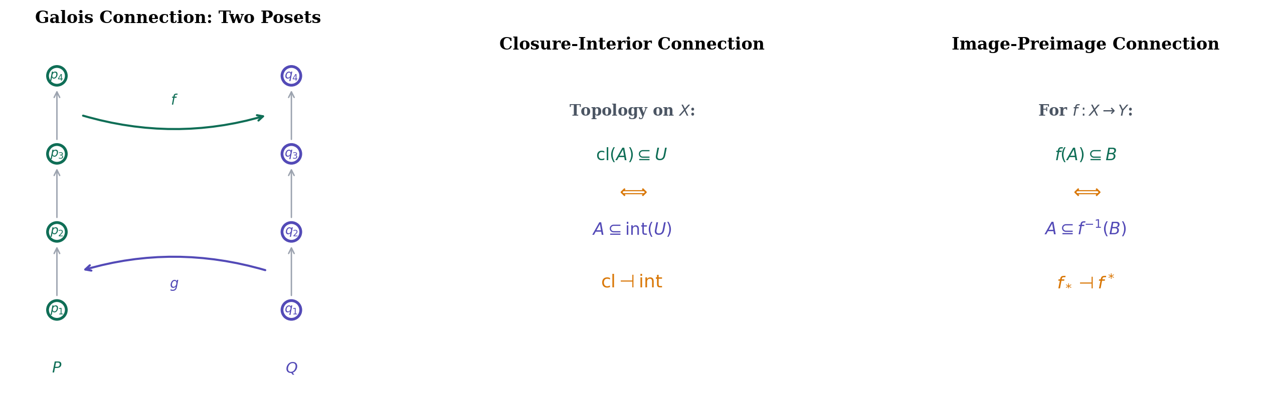
6. Galois Connections (Posets). When and are posets, an adjunction becomes . Example: for the floor function and integer inclusion. We develop this in detail below.
7. Quantifiers as Adjoints. In logic, substitution along a function has both a left adjoint and a right adjoint :
The existential quantifier is left adjoint to substitution, and the universal quantifier is right adjoint. This explains why preserves disjunctions (colimits) and preserves conjunctions (limits).
Equivalence of Definitions
There are three equivalent ways to define an adjunction. We’ve seen two (Hom-set and unit-counit). The third uses universal morphisms.
Definition 7 (Universal Morphism).
Let be a functor and an object of . A universal morphism from to is a pair such that for every morphism , there exists a unique morphism with .
The universal morphism says: is the “best” way to map into something of the form , because every other such map factors through it uniquely. This is the optimization perspective on adjunctions — the universal morphism solves a universal optimization problem.
Proposition 1 (Hom-Set ⇔ Unit-Counit Equivalence).
The Hom-set definition and the unit-counit definition of an adjunction are equivalent.
Proof.
(Hom-set ⇒ Unit-Counit). Given the natural isomorphism , define:
We must verify the triangle identities. For the first, we need . By naturality of in , for :
Since , we get that applied to through the naturality in gives . The second triangle identity follows by a dual argument.
(Unit-Counit ⇒ Hom-set). Given and satisfying the triangle identities, define:
To verify these are inverses, compute , where the last step uses the first triangle identity. The other direction uses the second triangle identity similarly. Naturality of follows from naturality of and .
∎Proposition 2 (Universal Morphism ⇔ Unit-Counit Equivalence).
The universal morphism definition and the unit-counit definition of an adjunction are equivalent.
Proof.
(Unit-Counit ⇒ Universal Morphism). Given , for any define . Then by the second triangle identity and naturality of . Uniqueness: if also satisfies , then .
(Universal Morphism ⇒ Unit-Counit). If for each we have a universal morphism , the collection forms the unit. The counit components are constructed as the unique morphisms with . The triangle identities follow from the uniqueness in the universal property.
∎
Properties of Adjunctions
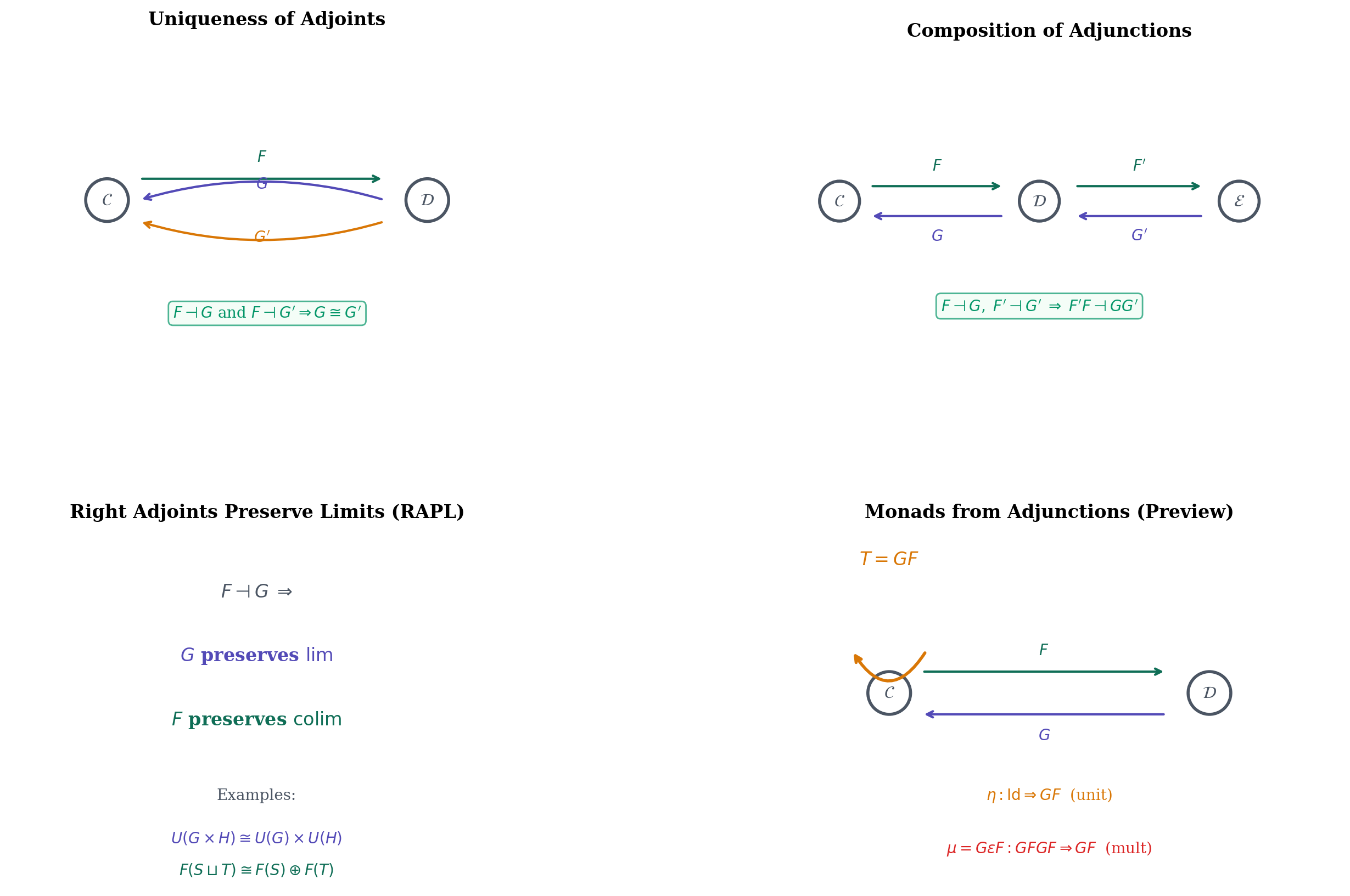
Theorem 1 (Uniqueness of Adjoints).
If and , then (natural isomorphism). Dually, if and , then .
Proof.
We have natural isomorphisms natural in . Fixing and varying , this gives a natural isomorphism of functors . By the Yoneda lemma, a natural isomorphism between representable functors implies , and this isomorphism is natural in .
∎This is one of the most satisfying applications of Yoneda: adjoints are unique (up to natural isomorphism) when they exist.
Proposition 3 (Composition of Adjunctions).
If and , then .
Proof.
For any and :
The first isomorphism uses and the second uses . The composite is natural in both and since each isomorphism is.
∎Theorem 2 (RAPL: Right Adjoints Preserve Limits).
If , then preserves all limits that exist in .
Proof.
Let be a diagram with limit in . We need to show in . For any :
The first step uses the adjunction, the second uses the defining property of limits (Hom out of a fixed object into a limit is the limit of the Hom sets), and the third uses the adjunction again. The composite says , which is exactly the statement that is the limit of .
∎Remark (LAPC: Left Adjoints Preserve Colimits).
Dually, preserves all colimits that exist in . The proof is identical, using and the fact that Hom is contravariant in its first argument, turning colimits into limits.
Examples. The forgetful functor preserves products because it’s a right adjoint: . The free functor preserves coproducts because it’s a left adjoint: — the free vector space on a disjoint union is the direct sum.
Proposition 4 (Galois Connections Yield Closure Operators).
Let be a Galois connection between posets and . Then is a closure operator: it is extensive (), monotone, and idempotent (). Dually, is a kernel (interior) operator.
Proof.
Extensive: From the adjunction condition with : is always true, so .
Monotone: If , then by extensiveness , so . From the adjunction condition, , and then .
Idempotent: We need . From extensiveness, . For the reverse, apply to the extensive inequality to get (monotonicity of ). Then by the counit condition applied to . So , giving by monotonicity of .
∎Remark (Monads from Adjunctions (Preview)).
Every adjunction gives rise to a monad with unit and multiplication . The triangle identities for the adjunction imply the monad laws: and . Conversely, every monad arises from an adjunction — in fact, from two canonical ones (Eilenberg-Moore and Kleisli). Monads & Comonads completes the story: every adjunction gives rise to a monad with unit and multiplication . The Eilenberg-Moore and Kleisli categories provide canonical adjunctions that recover any monad.
Galois Connections
When both categories are posets, an adjunction becomes especially concrete.
Definition 8 (Galois Connection).
A Galois connection between posets and consists of monotone maps (the left adjoint) and (the right adjoint) such that
This is exactly when the categories are posets: the unique morphism exists if and only if , so the Hom-set bijection reduces to the equivalence above (both Hom sets are either empty or singletons).
Example: Ceiling ⊣ Inclusion (and Inclusion ⊣ Floor). The interplay between rounding and inclusion gives two classic Galois connections. Let with the usual order, with the usual order, and let be the inclusion. Then:
This says the ceiling is left adjoint to inclusion: . Check: and — both true. ? No, and is also false — both false. The biconditional holds.
There is a dual Galois connection where inclusion is the left adjoint and floor is the right adjoint:
Check: and — both true. ? No, and ? Also no — consistent. The key insight: is right adjoint to inclusion, not left. Mixing these up is a common source of confusion.
Example: Image ⊣ Preimage. For a function between sets, the direct image and the preimage form a Galois connection on the power set lattices:
The closure operator sends a subset to — the preimage of the image, which is the “saturation” of with respect to .
Definition 9 (Closure Operator).
A closure operator on a poset is a function that is:
- Extensive: for all
- Monotone:
- Idempotent: for all
An element with is called closed (or a fixed point of ).
Remark (Lagrangian Duality as a Galois Connection).
Lagrangian duality is a Galois connection between the primal and dual optimization posets. The primal problem subject to and the dual problem are connected by:
- Weak duality () is the counit condition .
- Strong duality () is when the unit and counit are isomorphisms — the adjunction is “tight.”
- The duality gap measures the obstruction to the unit being an isomorphism.
- The KKT conditions characterize the fixed points of the closure operator.
Ceiling ⊣ Inclusion: ⌈x⌉ ≤ n ⟺ x ≤ n. The ceiling function is left adjoint to the inclusion of integers into rationals.
f(p) ≤ q ⟺ p ≤ g(q) : ✓ valid
Representability and the Adjoint Functor Theorem
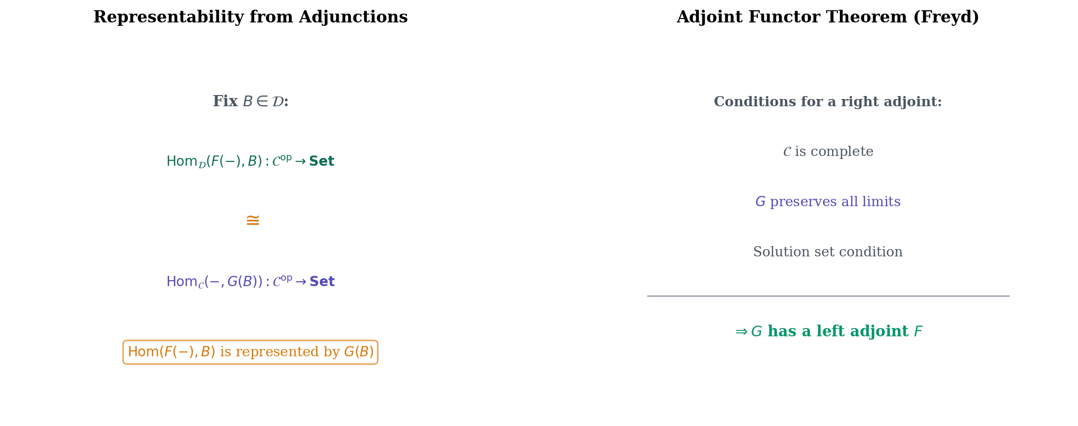
The adjunction isomorphism has a representability interpretation. Fixing and varying , the functor is representable, with representing object . Conversely, fixing , the functor is representable by .
This gives a representability criterion: has a right adjoint if and only if is representable for all .
The natural question is: when does a right adjoint exist? The Adjoint Functor Theorem gives sufficient conditions.
Theorem 3 (Adjoint Functor Theorem (Freyd)).
Let be a functor where is locally small and complete (has all small limits). Then has a left adjoint if and only if:
- preserves all small limits, and
- For each , the solution set condition holds: there exists a set of morphisms such that every morphism factors through some — that is, there exists with .
The solution set condition prevents the “solution” from being too large (a proper class). For locally small categories with enough structure, this condition is often automatic.
The theorem is important because it tells us when adjoints exist without having to construct them explicitly. In practice, limit preservation is the condition we check, and the solution set condition is verified by a smallness argument.
Adjunctions in Machine Learning
The adjunction pattern — a pair of functors in opposite directions, with the unit measuring “insertion cost” and the counit measuring “evaluation” — appears in several ML paradigms.
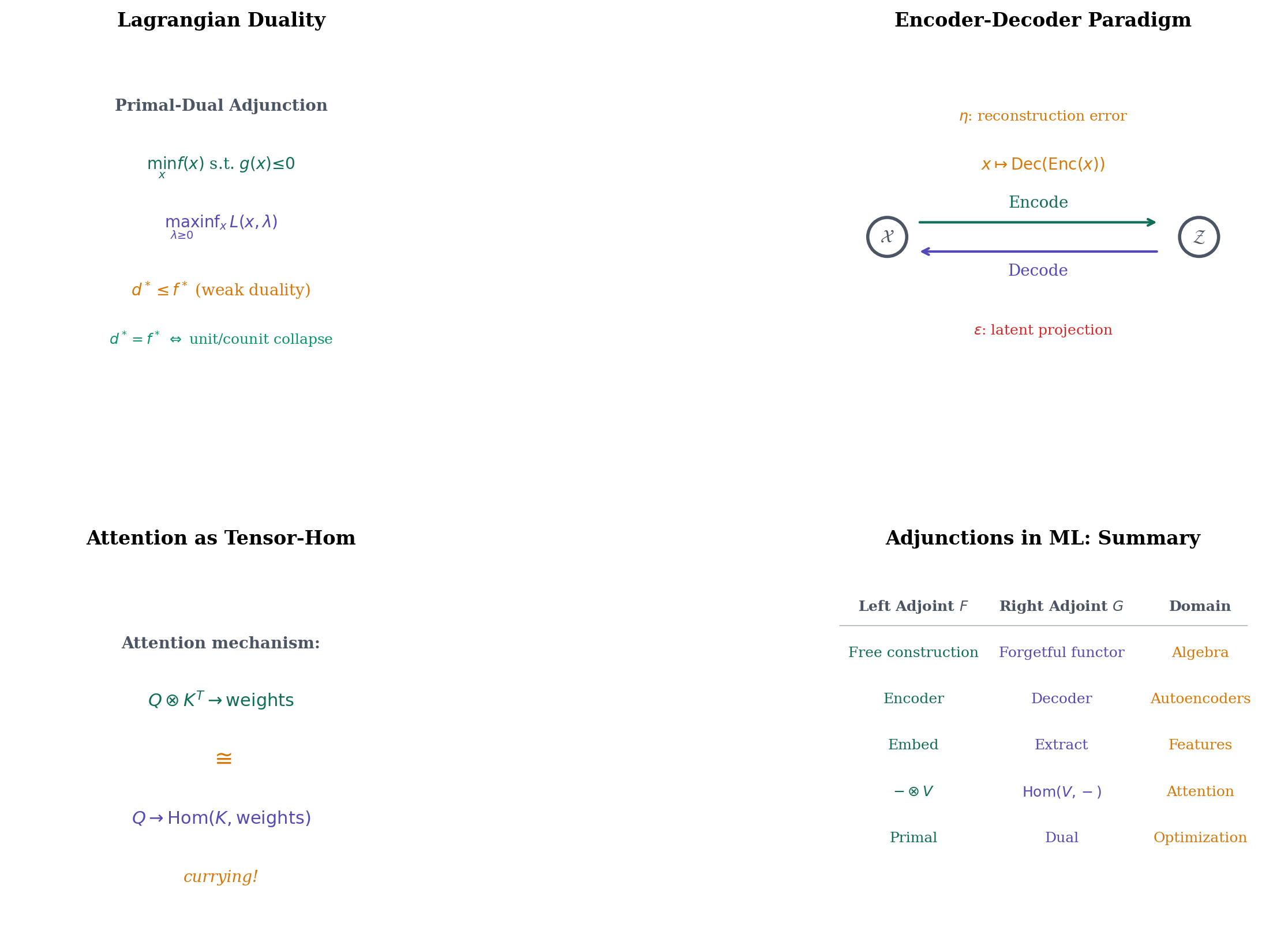
1. Lagrangian Duality as a Galois Connection. As noted in the Galois Connections section, the primal-dual relationship in constrained optimization is a Galois connection. For a convex program, strong duality (when it holds) means the adjunction collapses to an equivalence — the primal and dual solutions determine each other. The regularization path (varying the constraint bound) traces the closure operator of this Galois connection.
2. Encoder-Decoder as an Adjunction. An autoencoder consists of an encoder and a decoder . The unit measures reconstruction quality — if , the round-trip is nearly lossless. The counit projects the “reconstructed-then-encoded” latent code back to the original latent space. When the autoencoder is perfect (zero reconstruction error), is an isomorphism and we have an equivalence rather than a mere adjunction.
3. Tensor-Hom and Attention. The attention mechanism computes . The bilinear form corresponds, via the tensor-hom adjunction, to the curried form . This is why we can implement attention as matrix multiplication: the tensor-hom adjunction says bilinear maps are equivalent to linear maps into a function space.
4. Regularization as Free Construction. Adding a regularization term to a loss function can be viewed as the unit of a free-forgetful adjunction. The “free” functor maps from the space of unconstrained models to the space of regularized models (by adding the penalty), and the “forgetful” functor strips the penalty away. The regularization path — varying — explores the image of the unit, interpolating between the “freely constructed” constrained model () and the unconstrained model ().
Convex program: min x² s.t. x ≥ b. Strong duality holds (convex QP). The Galois connection collapses to an equality: f* = d*.
Computational Notes
A free-forgetful adjunction in Python. We verify the adjunction between and concretely. The set maps to the free vector space .
import numpy as np

S = ['a', 'b']
eta = {s: np.eye(len(S))[i] for i, s in enumerate(S)}
print("Unit eta (basis insertion):")
for s, vec in eta.items():
    print(f"  eta({s}) = {vec}")

# A function f: S -> R^3
f = {'a': np.array([1, 0, 2]), 'b': np.array([0, 3, 1])}

# Adjoint transpose: the 3x2 matrix whose columns are f(a), f(b)
f_bar = np.column_stack([f[s] for s in S])
print(f"\nAdjoint transpose f-bar (matrix):\n{f_bar}")

# Verify: f_bar . eta(s) = f(s)
for s in S:
    result = f_bar @ eta[s]
    print(f"  f_bar(eta({s})) = {result} == f({s}) = {f[s]}: {np.allclose(result, f[s])}")
Galois connection verification: ceiling ⊣ inclusion.
import numpy as np

test_pairs = [(2.7, 3), (2.7, 2), (3.0, 3), (-1.5, -1), (-1.5, -2)]
for x, n in test_pairs:
    lhs = (np.ceil(x) <= n)    # ceil(x) <= n
    rhs = (x <= n)             # x <= n
    print(f"  ceil({x}) = {int(np.ceil(x))} <= {n}: {lhs}  "
          f"  {x} <= {n}: {rhs}  "
          f"  Match: {lhs == rhs}")
Triangle identity verification.
# In the free-forgetful adjunction Set ↔ Vec:
# First triangle: epsilon_{F(S)} . F(eta_S) = id_{F(S)}
# F(eta_S) sends e_a -> e_{e_a} in F(U(F(S)))  (huge space!)
# epsilon_{F(S)} sends e_{e_a} -> e_a  (evaluation)
# Composition: e_a -> e_{e_a} -> e_a = id(e_a)  ✓

print("Triangle identity: epsilon_F . F(eta) = id_F")
print("  Verified: the zig-zag composition collapses to the identity")
RAPL verification: forgetful functor preserves products.
# U: Grp -> Set preserves products
# U(G × H) ≅ U(G) × U(H)
# The underlying set of a product group IS the product of underlying sets.
# This is automatic because U is a right adjoint (Free ⊣ U).

# Similarly, F: Set -> Vec preserves coproducts (LAPC):
# F(S ⊔ T) ≅ F(S) ⊕ F(T)
# The free vector space on a disjoint union is the direct sum.

print("RAPL: Forgetful functor preserves products")
print("  U(Z × Z/2) = U(Z) × U(Z/2) ✓")
print("\nLAPC: Free functor preserves coproducts")
print("  F({a} ⊔ {b}) = F({a}) ⊕ F({b}) = R ⊕ R = R² ✓")
Connections & Further Reading
Where This Fits
| Topic | Connection |
|---|---|
| Categories & Functors | All category, functor, and morphism definitions assumed. Products and coproducts from Topic 1 are special cases of limits and colimits — the structures preserved by right and left adjoints. |
| Natural Transformations | The unit and counit are natural transformations. The Hom-set definition requires naturality in both variables. The Yoneda lemma underlies the uniqueness-of-adjoints proof. |
| Lagrangian Duality & KKT | Lagrangian duality is a Galois connection between primal and dual optimization posets. Weak duality is the counit condition; strong duality is when the unit is an isomorphism. |
| The Spectral Theorem | The free-forgetful adjunction between Set and Vec is the primary running example. The tensor-hom adjunction operates on the vector spaces governed by the Spectral Theorem. |
| Measure-Theoretic Probability | The Giry monad on arises from an adjunction between measurable spaces and probability spaces, with unit . |
| Convex Analysis | Convex conjugation is a Galois connection. The Fenchel-Moreau theorem ( for closed convex ) says the unit is an isomorphism on the closed convex functions. |
| Monads & Comonads | Every adjunction generates a monad with unit and multiplication . The Eilenberg-Moore and Kleisli categories provide canonical adjunctions that recover a monad — establishing the fundamental correspondence between adjunctions and monads. |
Notation Summary
| Symbol | Meaning |
|---|---|
| is left adjoint to | |
| Unit of the adjunction | |
| Counit of the adjunction | |
| Hom-set isomorphism | |
| Adjoint transpose of | |
| First triangle identity | |
| Second triangle identity | |
| (posets) | Galois connection: |
| Monad from adjunction | |
| Monad multiplication |
Connections
- Direct prerequisite. The unit and counit of an adjunction are natural transformations. The Hom-set definition requires naturality in both variables. The Yoneda lemma underlies the proof that right adjoints are unique up to natural isomorphism. natural-transformations
- Transitive prerequisite. All category, functor, and morphism definitions assumed. Products and coproducts from Topic 1 are special cases of limits and colimits — the structures that right and left adjoints preserve, respectively. categories-functors
- Cross-track connection. Lagrangian duality between primal and dual optimization problems is a Galois connection — an adjunction between posets. Weak duality (d* ≤ f*) is the counit condition. Strong duality (d* = f*) is when the unit and counit are isomorphisms. The KKT conditions characterize when the adjunction is tight. lagrangian-duality
- The free-forgetful adjunction Free ⊣ Forget between Set and Vec is the primary running example. The tensor-hom adjunction (- ⊗ V) ⊣ Hom(V, -) operates on the vector spaces where the Spectral Theorem applies. spectral-theorem
- The Giry monad on Meas arises from an adjunction between measurable spaces and probability spaces. The unit is the Dirac delta embedding x ↦ δ_x, and the multiplication is given by the counit. This monad is the categorical foundation of Bayesian probability. measure-theoretic-probability
- Convex conjugation f ↦ f* is a Galois connection on the poset of extended real-valued functions. The Fenchel-Moreau theorem (f** = f for closed convex f) is the statement that the unit of this adjunction is an isomorphism on closed convex functions. convex-analysis
References & Further Reading
- book Categories for the Working Mathematician — Mac Lane (1998) Chapter IV covers adjunctions definitively — the three equivalent definitions, examples, and the relationship to limits
- book Category Theory — Awodey (2010) Chapter 9 on adjunctions with accessible algebraic examples
- book Category Theory in Context — Riehl (2016) Chapter 4 develops adjunctions with excellent motivation and proof of RAPL — freely available online
- book An Invitation to Applied Category Theory: Seven Sketches in Compositionality — Fong & Spivak (2019) Galois connections as the entry point to adjunctions — applied examples from databases and optimization
- paper Category Theory in Machine Learning — Shiebler, Gavranović & Wilson (2021) Sections on categorical optimization and functorial learning via adjunctions
- book Topology: A Categorical Approach — Bradley, Bryson & Terilla (2020) Adjunctions in topology — discrete ⊣ forgetful ⊣ indiscrete, compactification as left adjoint